Gradient Feature-Based Collaborative Filtering in Verification Federated Learning with Privacy-Preserving

1  Introduction

1.1 Background

Although one of the key advantages of FL is the ability to train models without exchanging original data, thereby preserving user privacy, gradients themselves can also leak sensitive information. Gradients contain information about the training data, and attackers might use this information to infer the original data, meaning that even without directly exchanging data, the transmission of gradients could potentially reveal specific user information [1]. In addition to direct data leakage, attackers can also launch model attacks using gradients, such as membership inference attacks or attribute inference attacks [2,3]. To address the issues mentioned above, some techniques like differential privacy [4,5] and homomorphic encryption [6] have been introduced into federated learning to prevent the leakage of user information through model gradient parameters.

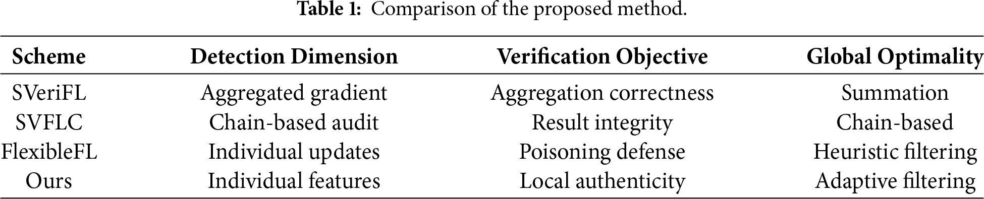
On the other hand, some clients involved in the federated learning process may not be entirely trustworthy. Certain clients might adopt a “free-riding” strategy, benefiting from the model improvements achieved through the data and computational resources contributed by other participants, while failing to make any meaningful contributions to the collaborative training process. Specifically, such free-riding clients might submit inaccurate, irrelevant, or fabricated model gradients, yet still utilize the final trained model for prediction or decision-making once it is publicly released [7,8]. Some malicious clients could deliberately submit erroneous or tampered gradients to disrupt the training process, potentially resulting in a degradation of model performance or even complete failure [9,10]. Additionally, in some scenarios, malicious servers might return incorrect results to users. For instance, “lazy” servers could compress the original model with a simplified and less accurate alternative to minimize their computational overhead, or they might maliciously alter the aggregated results before transmitting them to users [11]. To mitigate the aforementioned issues, various techniques have been employed to verify the correctness of aggregated gradients, including Lagrange interpolation [12,13], cryptographic signatures [14], commitments [15], and zero-knowledge proofs [16,17]. However, these methods only focus on whether the aggregated gradient is correctly processed and verified, rather than whether each user has honestly trained locally, and it is still possible for users to adopt a “free-riding” strategy or engage in malicious behaviors by submitting forged gradients without being directly detected. To further clarify the distinctive contributions of our proposed scheme, we provide a structured comparison with verifiable FL frameworks: FlexibleFL [18], SVeriFL [19] and SVFLC [20] in Table 1. As summarized in the table, while existing works primarily focus on ensuring that the server performs honest aggregation, our work shifts the emphasis toward verifying the integrity of the local training process itself. By employing JL-projection for dimensionality reduction and collaborative filtering for similarity-based detection, our scheme achieves more granular detection of malicious behaviors that are often overlooked by purely cryptographic verification methods.

1.2 Contribution

To address the above issues, we propose a gradient feature-based collaborative filtering (CF) [21,22] scheme in verificatiCon federated learning to ensure the effectiveness and security of distributed model training. In our scheme, the storage-assisted server (SAS) is used to monitor whether the user and aggregation server (AS) are honestly implementing the training protocol to ensure that the entities participating in model training are complying with their protocol during training. Our contribution can be summarized as follows:

•   We introduce a collaborative filtering (CF) mechanism based on gradient features for verifiable federated learning. Unlike prior approaches relying solely on direct gradient similarity, our method applies JL-type gradient dimensionality reduction to construct a unified, structure-preserving behavior space, enabling CF to capture multi-user behavioral patterns more effectively. This combination of CF with projected gradient representations provides a richer and more robust basis for detecting abnormal or dishonest updates.

•   To detect potentially malicious behavior from users or the aggregation server, we design a monitoring mechanism centered on the SAS, which evaluates the consistency between masked gradients and aggregated gradients. The SAS leverages the projected behavioral features uploaded by clients to monitor the execution of the protocol and allows honest entities to verify the correctness of aggregation without exposing raw gradients.

•   To demonstrate the effectiveness of our scheme, we perform a detailed security analysis showing resilience against integrity-related threats. We further evaluate its practical utility through comprehensive experiments on two real-world datasets, confirming the robustness and efficiency of our framework under diverse settings.

1.3 Organization

The remainder of the paper is organized as follows. In Section 2, we provide an overview of our proposed system model. In Section 3, we elaborate on our gradient feature-based collaborative filtering scheme. Experimental comparisons and analysis are conducted in Section 4. Section 5 discusses limitations and future research directions. Finally, Section 6 summarizes this paper.

2  System Overview

2.1 System Model

The proposed system model is including three key entities: trusted authority, users involved in the training and servers. The servers are further categorized into two types: the aggregation server and the storage-assisted server. The detailed functions of these three entities are defined as follows:

Trusted Authority (TA): TA is responsible for generating and distributing the parameters required for each training round. In the training process, TA handles the removal of masks from the global gradient after unmasking, and it then generates and distributes the updated global gradient along with the corresponding mask matrix for the next training round. By calculating the sum of all users’ masks, TA is able to remove the mask from the aggregated result, thereby ensuring the accurate aggregation of these gradients. TA is fully trusted and is responsible for generating the random projection matrix R, per-round dynamic mask matrices, and cryptographic parameters. TA does not access any gradients, masked gradients, or verification materials.

AS and SAS: AS is responsible for receiving the local gradients from each user and aggregating the local gradients. Also, SAS is responsible for supervising the above aggregation process, including verifying whether the AS is honest about the aggregation results and whether the users are honest about their training. The SAS also informs those entities of its detection results. AS may be malicious and can alter, drop, or forge user updates, but it receives only masked gradients and never obtains R or mask components. SAS is honest-but-curious; it only receives projected gradients and projected masks for verification but does not participate in aggregation or hold any secret keys.

Users: Users are training participants in the federated learning process, that can possess local training data. They actively request federated learning training tasks, train their local models for each round using their local data, and send their masked local models to the AS for model aggregation.

We assume that no two entities collude, and neither AS nor SAS receives a complete mask vector. This non-collusion model ensures that no single server can recover user gradients or simultaneously manipulate both aggregation and verification paths.

2.2 Security Concerns and System Objective

Under the proposed system model, we assume that a TA is completely trustworthy and does not collude with any user or server (similar settings can be found in the paper [23]). The AS is considered to be malicious and endeavors to collude with other users to gain access to their original models, thereby inferring their original data and compromising their private information. To alleviate the workload, the AS may selectively aggregate only a subset of models or maliciously forge the aggregation results. Subsequently, these incorrect aggregated outputs are provided to the trainers. Also, the SAS is characterized by both honesty and curiosity: it adheres to executing all protocol steps meticulously, while also being inquisitive about the data provided by other users. Further, users may employ the “free-riding” tactics, leveraging historical local gradients to alleviate their computational burden, but we assume the overall training system is composed of more users who engage in honest training than those who resort to free-riding. Additionally, some users might endeavor to deduce the private information of others. Therefore, our security objective is to maintain the effective oversight of user training throughout the federated learning process and ensure the stringent protection of user security. We acknowledge that the assumption of a fully trusted TA and an honest-but-curious SAS may not always hold in all real-world deployments. However, these assumptions are widely adopted in verifiable and privacy-preserving FL frameworks, and enable our scheme to focus on robustness and integrity without introducing additional cryptographic interaction overhead.

2.3 Design Goal

To clearly separate the protection goals addressed by our framework, we distinguish three security objectives: robustness, integrity, and privacy, and map each objective to the system component responsible for achieving it.

(1) Robustness: SAS is responsible for robustness-related verification. It receives only projected gradient features and projected masks, and performs collaborative-filtering–based analysis to determine whether a user behaves as a free-rider or uploads forged updates. The verification relies on checking temporal consistency of gradients, similarity among peers in the projected space, and the coherence between each projected gradient and its corresponding projected dynamic mask. These operations jointly enable robustness against dishonest users without exposing any raw gradient information.

(2) Integrity: AS aggregates masked gradients but does not participate in verification. Users and SAS independently generate verification materials based on the dynamic mask scheme. This separation ensures that a malicious AS cannot forge or manipulate aggregation results without being detected by the SAS, thereby guaranteeing the integrity of the global update.

(3) Privacy: TA distributes per-round dynamic mask matrices that hide user gradients from both AS and SAS. Random projection reduces the dimensionality of gradient representations and limits the amount of detailed structure exposed to the verifier, while approximately preserving distance relationships useful for similarity-based detection. We stress that projection is not a cryptographic privacy mechanism. Together, the masking and projection components ensure that user gradients remain unlinkable and unrecoverable across rounds.

Clarification on the role of random projection. We emphasize that random projection in our scheme is used for dimensionality reduction and to preserve pairwise similarity structure in a compact form for efficient collaborative-filtering based detection. It is not intended as a cryptographic privacy mechanism nor does it, by itself, provide formal privacy guarantees. The principal privacy protection is achieved by the per-round dynamic masking scheme; projection only reduces the exposed feature dimensionality and may empirically limit fine-grained leakage.

Scope clarification. We note that differential privacy (DP) is not included in our threat model. Our scheme operates under a masking-based privacy protection setting and focuses on verifying the correctness of client updates and detecting dishonest users. DP provides a separate layer of formal privacy guarantees through calibrated noise injection, which is orthogonal to the verification objective addressed in this work. Integrating DP as an additional privacy mechanism is possible, but is beyond the scope of this paper and is left for future work.

3  Proposed Scheme

As shown in Fig. 1, our gradient feature-based collaborative filtering scheme is divided into five phases, which includes system initialization, model training and upload, user gradient anomaly detection, gradient aggregation and aggregation result verification. Based on the proposed system model, our gradient feature-based collaborative filtering scheme with privacy-preserving is divided into five phases, which includes system initialization, model training and upload, user gradient anomaly detection, gradient aggregation and aggregation result verification. The detailed collaborative filtering process is shown in Fig. 2.

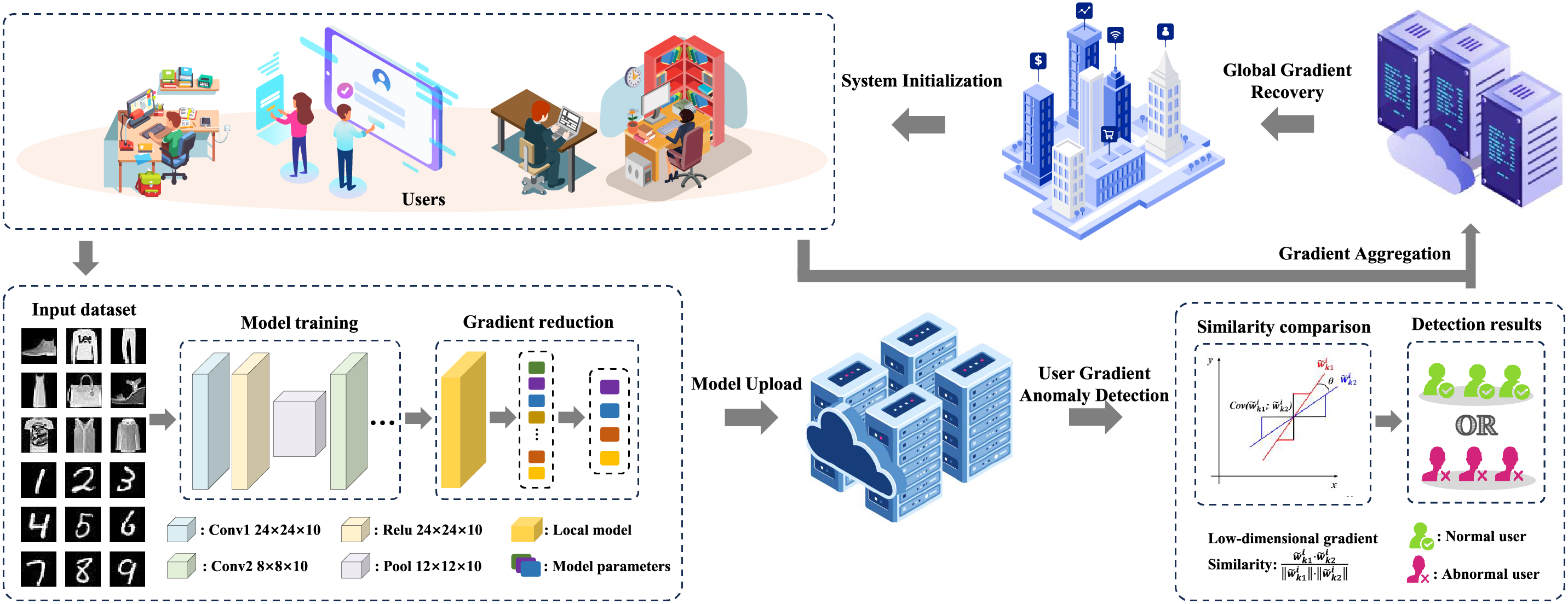
Figure 1: System model.

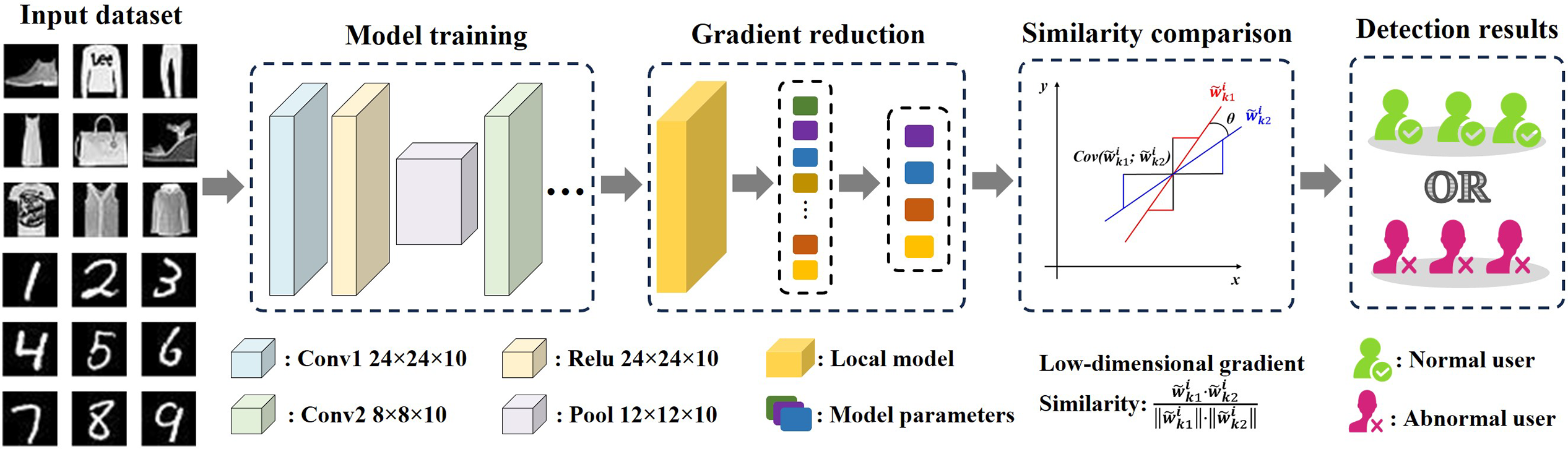
Figure 2: Collaborative filtering process.

3.1 System Initialization

In the system initialization phase, TA executes parameter configurations. The TA receives task requests and registration details from all participating users (assuming a total of n users), thereby forming a set of training users denoted as U. Subsequently, the TA randomly selects two servers with adequate computational resources to act as the aggregation server (AS) and the secure aggregation server (SAS) for the aggregation task, where we assume the TA can construct secure communication channels with all entities involved. Following this, the TA generates n random masks (m1i,m2i,m3i,…,mni) and computes the total mask value locally as Mi=1n∑k=1nmki. To ensure security, mki and Mi are dynamically regenerated in each training round. Additionally, the TA generates a random projection matrix to map high-dimensional gradients into a lower-dimensional feature space. This projection approximately preserves pairwise distances in expectation and reduces representation dimensionality for downstream detection. The TA also sets initial global model parameters wgi, along with other training parameters such as batch size B, learning rate η, local iteration count E, and global iteration count δ. Furthermore, the TA selects cyclic groups G1 and G2, where g and h are used as the bilinear pairing generators, and q represents the prime order of the finite field. The bilinear pairing map is defined as e:G1×G2→GI. After initializing the parameters, the TA sends these initial parameters to each entity.

3.2 Model Training and Upload

After the TA completes the system initialization process, each user performs it local training using the global model parameters wgi received from the TA. The users calculate the loss function based on their own dataset and update their local model parameters to wki:

wki+1←wgi−η∇Lf(Dk,wgi).(1)

To ensure data security during the upload process, the users mask their local gradients w^ki by adding the mask mki provided by the TA:

w^ki=wki+mki.(2)

Subsequently, each user computes the local verification value verifyki based on the masked gradient and the mask:

verifyki=e(gwki,hmki)modq.(3)

This verification value will be used to validate the honest operation of the AS. Additionally, each user maps (or reduces) its local gradients to a low-dimensional feature vector w~ki using the random matrix provided by the SAS for subsequent anomaly detection. And each user also computes the low-dimensional mask vector m~ki for the honesty upload detection phase:

w~ki=RTwki.(4)

Although SAS receives both the projected gradients RT(wki+mki) and the masks RTmki gradient privacy remains preserved for two reasons. First, the JL-type projection with r≪d is intrinsically non-invertible; infinitely many original gradients correspond to the same low-dimensional projection. Second, the dynamic masks are refreshed every round, making projected values unlinkable across iterations. Consequently, SAS cannot reconstruct or approximate the original gradient structure beyond the coarse similarity information intentionally retained for collaborative filtering–based detection. We explicitly note that projection alone does not provide formal privacy guarantees, and such formal guarantees are outside the scope of this work. After completing these data calculations, each user sends the low-dimensional feature gradient w~ki, the low-dimensional mask vector m~ki, and the verification value verifyki to the SAS. Additionally, each user sends the masked gradient w^ki to the AS. The specific details of this phase are outlined in Algorithm 1. Inspired by the Johnson-Lindenstrauss Lemma [24], the following lemma holds.

Lemma 1: For any two gradient vectors wk1i,wk2i∈Rd, a random projection matrix R∈Rd×r can approximately preserve their distance. The columns of R are random vectors with elements Rij∼𝒩(0,1r), independently and identically distributed. When R satisfies the independence and randomness conditions, the following holds:

(1−ε)‖wk1i−wk2i‖2≤‖RT(wk1i−wk2i)‖2≤(1+ε)‖wk1i−wk2i‖2(5)

where ε∈(0,1) depends on the projection dimension r and the number of points n, ensuring the projected distances are approximately preserved.

Proof: For the gradient difference between users uk1 and uk2:

x=wk1i−wk2i,(6)

we need to analyze the properties of its projection RTx. Since the columns of R are independent and identically distributed, with Rij∼𝒩(0,1r), the squared distance after projection can be written as:

‖RTx‖2=∑k=1r(∑j=1dRjkxj)2.(7)

For the expectation of ‖RTx‖2, since Rij∼𝒩(0,1r), a normal random variable with mean 0, its variance is:

Var(∑j=1dRjkxj)=∑j=1dxj2⋅1r=‖x‖2r.(8)

Therefore, ∑j=1dRjkxj∼𝒩(0,‖x‖2r). Its square (∑j=1dRjkxj)2 is a scaled chi-square random variable. Specifically:

(∑j=1dRjkxj)2∼‖x‖2r⋅χ2(1),(9)

where χ2(1) is a chi-square distribution with 1 degree of freedom, having expectation 1 and variance 2. Thus:

E[(∑j=1dRjkxj)2]=‖x‖2r⋅1=‖x‖2r.(10)

Summing over all r dimensions, we get:

E[‖RTx‖2]=∑k=1rE[(∑j=1dRjkxj)2]=∑k=1r‖x‖2r=‖x‖2.(11)

This indicates that the expectation of the squared distance after projection equals the squared original distance, meaning that random projection preserves the distance in expectation. Next, we calculate the variance of ‖RTx‖2. Let Zk=∑j=1dRjkxj, then ‖RTx‖2=∑k=1rZk2. Since the columns of R are independent, the Zk are also independent. Each Zk∼𝒩(0,‖x‖2r), and its square Zk2∼‖x‖2r⋅χ2(1). The variance of the chi-square distribution χ2(1) is 2, so:

Var(Zk2)=(‖x‖2r)2⋅2.(12)

The total variance is:

Var(‖RTx‖2)=∑k=1rVar(Zk2)=r⋅2(‖x‖2r)2=2‖x‖4r.(13)

The variance is inversely proportional to the projection dimension r, indicating that a larger r results in a smaller variance and thus a more concentrated projected distance. To quantify the approximation error, we use Chebyshev’s inequality. Let Y=‖RTx‖2, with expectation E[Y]=‖x‖2 and variance Var(Y)=2‖x‖4r. According to Chebyshev’s inequality:

P(|Y−E[Y]|≥ εE[Y])≤Var(Y)(εE[Y])2.(14)

Substituting the values:

P(|Y−‖x‖2|≥ ε‖x‖2)≤2‖x‖4r(ε‖x‖2)2=2rε2.(15)

This shows that the probability that the projected distance deviates from the original distance by more than  ε‖x‖2 is at most 2rε2, i.e.,

P((1− ε)‖x‖2≤‖RTx‖2≤(1+ε)‖x‖2)≥1−2r ε2.(16)

Therefore, with a sufficiently large projection dimension r, making 2r ε2 small, the projected distance will lie within (1 ± ε)‖x‖2 with high probability. If we require this probability to be less than a small error probability δ, then:

2rε2≤δ ⟹ r≥2δε2.(17)

This indicates that to ensure the projected distance lies within (1 ± ε)‖x‖2 with probability at least 1−δ, the projection dimension r needs to satisfy r=Ω(1δ ε2). ◻

3.3 User Gradient Anomaly Detection

After the SAS receives the low-dimensional feature vectors w~ki uploaded by all the users, it calculates a collaborative filtering embedding feature vector Eki for each user:

Eki=α⋅(w~ki−w~ki−1)+β⋅(w~ki−w~j∗i).

This vector encapsulates the changes in the user’s local feature gradient relative to the historical gradients and the global gradient. Using these user collaborative filtering embedding feature vectors, the SAS constructs a user gradient behavior matrix Hi. Once the construction is complete, the SAS employs a random sampling method to compare each user’s feature vector with randomly selected feature vectors from other users, calculating similarity scores to detect anomalies in user gradients. To identify whether users or the AS are fabricating gradient information or utilizing outdated historical gradient data for continued training, we propose a user gradient anomaly detection method based on the Johnson-Lindenstrauss Lemma and collaborative filtering (CF) mechanism. In addition, we employ the Top-q Sign Fingerprint (TSF). For each user uk, let Tq(w~ki) denote the index set of the top-q coordinates of w~ki ranked by absolute value:

Tq(w~ki)={p1,p2,…,pq},(18)

where each pt is a coordinate index. The sign function for coordinate p is defined as

sign(w~k,pi)={+1,w~k,pi≥0,−1,w~k,pi<0.(19)

The TSF similarity between users uk and uj is then given by:

TSF(w~ki,w~ji)=|{p∈Tq(w~ki)∩Tq(w~ji):sign(w~k,pi)=sign(w~j,pi)}|q.(20)

If Tq(w~ki)∩Tq(w~ji)=∅, then TSF=0. When the intersection Tq(w~ki)∩Tq(w~ji) is empty or very small, TSF is defined as 0 to avoid undefined values. This value lies in [0,1], where higher values indicate a greater degree of sign consistency on the most important coordinates between two users. The most similar user of uk is determined as:

j∗=arg⁡maxj≠kTSF(w~ki,w~ji).(21)

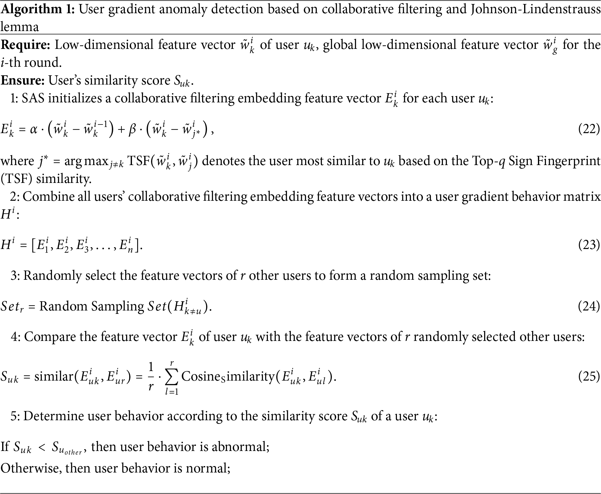
The specific details of this phase are summarized in Algorithm 1. The schematic process of user abnormal behavior detection based on collaborative filtering is shown in Fig. 3. Based on this process, the following theorems hold:

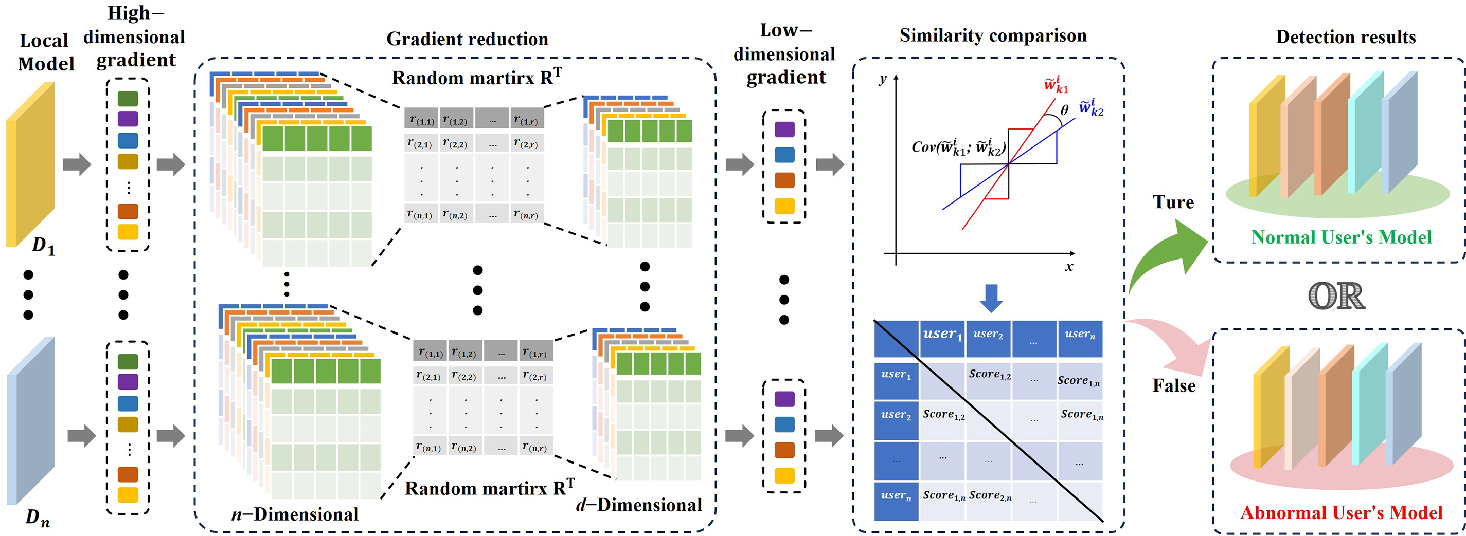
Figure 3: Johnson-Lindenstrauss Lemma schematic.

Theorem 1: (Rationality analysis of embedded features and similarity score): In our scheme, the embedded feature vector Eki is expressed as follows:

Eki=α⋅(w~ki−w~ki−1)+β⋅(w~ki−w~j∗i),

which combines low-dimensional local gradient variation and peer difference derived from the most similar user, effectively characterizing user behavioral features. Additionally, the similarity score Suk accurately captures anomalous behaviors, enabling user anomaly detection.

Proof: The embedded feature vector Eki consists of two components, each capturing a different behavioral dimension. The first component, the local gradient variation w~ki−w~ki−1, reflects the change in local gradients between consecutive rounds. For honest users, this difference tends to be smooth and consistent, with its distribution concentrated away from zero. However, if a user uploads outdated gradients, the term becomes zero, indicating stagnation. Conversely, fabricated gradients may cause sudden and irregular changes, leading to significant deviations. This component thus serves as an indicator of temporal continuity and behavioral stability across rounds. The second component, the peer difference w~ki−w~j∗i, measures how well a user’s local update aligns with that of its most similar peer identified by the TSF similarity. Honest users typically share similar update directions with their close peers, resulting in small deviations. In contrast, malicious or extremely deviating users tend to produce updates that diverge strongly from their peer’s direction, even when their local change appears normal. This dual design ensures that any anomaly triggers detectable deviations in at least one component. The combined feature Eki thus simultaneously monitors temporal consistency and peer-level behavioral conformity. Cosine similarity is then used to evaluate directional alignment between feature vectors:

Suk=similar(Euki,Euri)=1r⋅∑l=1rCosine_Similarity(Euki,Euli)<Suother

where Suother is the median similarity score of all users, the detection rule is defined as: if Suk<Suother, uk exhibits abnormal behavior. During the aggregation phase, gradients from user uk are explicitly excluded based on our anomaly detection criteria. ◻

Theorem 2: (Effectiveness of collaborative filtering in detecting user behavior matrix similarity differences): In our scheme, a user’s honest training behavior can be monitored and evaluated based on its behavior score and the user gradient behavior matrix Hi:

Hi=[E1i,E2i,E3i,…,Eni],

where each embedded feature vector Eki integrates both local gradient variation and peer difference derived from the most similar user. By converting user behavior into numerical vectors and constructing the collaborative filtering matrix, the SAS can effectively monitor and analyze user training behavior patterns.

Proof: The behavior score Suk of user uk is computed by randomly selecting k users and comparing the cosine similarity of their low-dimensional embedded feature vectors. Let Un denote the number of normal users and Ua the number of abnormal users, where Un+Ua=N, and N is the total number of users. To ensure that the behavior scores of normal users remain higher than those of abnormal users, the number of normal users must exceed the number of abnormal users. Specifically, for a normal user, the number of its comparisons with other normal users should be greater than that with abnormal users. Thus, when at least (k2+1) normal users are compared, the minimum probability that a normal user’s score is positive can be expressed as:

Probabilityn=(Un−1N−1)⋅(Un−2N−2)⋯(Un−(k2+1)N−(k2+1))=∏i=0k2+1Un−iN−i.(26)

For an abnormal user whose score is positive, the probability is:

Probabilitya=(Ua−1N−1)⋅(Ua−2N−2)⋯(Ua−(k2−1)N−(k2−1))=∏i=0k2−1Ua−iN−i.(27)

When Probabilityn>Probabilitya, the overall scoring mechanism can effectively distinguish between normal and abnormal users. Therefore, the collaborative filtering mechanism, by leveraging the similarity among user gradient behavior features derived from Eki, can reliably perform user anomaly detection. ◻

3.4 Gradient Aggregation

After the SAS completes the anomaly detection of user gradients, it needs to verify whether the user masking gradient received by the AS is consistent with the gradient source of the low-dimensional feature gradient uploaded by each user and verified by the SAS. To achieve this, the SAS utilizes the previously uploaded low-dimensional feature gradient vector w~ki and the user low-dimensional feature mask vector m~ki. Upon receiving the user masking gradient m^ki, the AS must calculate the low-dimensional feature of the masking gradient RTw~ki and upload it to the SAS. Subsequently, the SAS calculates the sum of w~ki and m~ki and determines whether the RTw^ki and (w~ki+m~ki) are equal:

RTw^ki=?w~ki+m~ki.(28)

If the verification is passed, then it indicates that the user has honestly uploaded the masked gradient. Next, the AS collects and aggregates the masked local gradients w^ki from each user:

w^gi=1n∑k=1nw^ki.(29)

To ensure the honest execution of the protocol and successful completion of the aggregation operation, the AS must correctly process the data uploaded by users. Upon receiving the masked gradients calculated by users during local training, the AS performs the gradient aggregation operation to generate the masked global gradient w^gi. After the global gradient aggregation is completed, the AS needs to send the aggregated masked global gradient to the SAS. Since verification materials are independently generated by each user and transmitted directly to SAS, the AS cannot alter or suppress them. SAS verifies both the per-user update behavior and the final aggregated gradient using these user-provided commitments. Therefore, even if AS is malicious, it cannot forge a valid aggregation result without being detected by SAS, as the computation paths of aggregation and verification are completely separated.

Theorem 3: (Detection correctness of user honesty upload): In our scheme, if the user honestly uploads its masking gradient and authentication information and the AS can honestly calculate the value of RTw^ki:

RTw^ki=?w~ki+m~ki,

then the correctness of the user uploading the masking gradient can be verified.

Proof: In the aggregation phase, it is necessary to verify whether the masked gradient w^ki uploaded to the Aggregation Server (AS) and the low-dimensional feature gradient vector w~ki uploaded to the Secondary Authentication Server (SAS) originate from the same source gradient, namely the raw training gradient wki. Since SAS stores both w~ki and m~ki, which are computed by projecting the user’s original gradient vector and the masking vector through a random matrix R, these values have previously been used to verify the user’s honest participation in training. Simultaneously, users are required to upload the masked gradient w^ki to AS for aggregation. To verify the consistency, AS can use the same random matrix R to project the masked local gradient w^ki and compare it with the verification information uploaded to SAS. The consistency condition is:

RTw^ki=RT(wki+mki)=?w~ki+m~ki,

where w~ki=RTwki and m~ki=RTmki. If the equation holds, it proves that the user has honestly uploaded the correct masked gradient based on their genuine training process. However, if the computed value RTw^ki does not match w~ki+m~ki, it indicates a mismatch between the masked gradient uploaded to AS and the verification information uploaded to SAS. This inconsistency implies dishonest behavior by the user, and consequently, the masked gradient w^ki will be excluded from the aggregation phase. ◻

3.5 Aggregation Result Verification Phase

To verify whether the AS has honestly executed the protocol and completed the aggregation operation, the SAS can verify the correctness of the aggregation performed by the AS using only the global masked gradient and the masked gradient verification values uploaded by each user. When the SAS receives the verification value verifyki calculated by each user during local training and the masked global gradient aggregated by the AS, it proceeds with the verification of the aggregation result:

verifyaggi=∏k=1ne(gwki,hmki)modq.(30)

Specifically, the SAS receives the masked global gradient w^gi sent by the AS, SAS calculates the verification value verifycalculatei on the masked global gradient:

verifycalculatei=e(gw^gi,h)modq.(31)

Then, SAS only needs to compare whether verifyaggi and verifycalculatei are the same to determine whether AS is integrity aggregation.

Theorem 4: (Correctness of Verifying the Global Gradient Aggregation Result): In our proposed scheme, if the AS honestly executes the global aggregation operation and correctly computes the masked global gradient w^gi, then the verification value verifycalculatei computed by the SAS will match the aggregated verification value verifyaggi derived from all users:

verifycalculatei=verifyaggi=∏k=1ne(gwki,hmki) mod q.(32)

Therefore, SAS can correctly determine whether the AS has honestly performed the aggregation. If the AS deviates from the protocol or returns an incorrect aggregation result, the above equality does not hold, and the verification consequently fails.

Proof: In the verification phase, our objective is to verify whether the following equation holds:

verifycalculatei=?verifyaggi.(33)

So, when the SAS calculates the verification value verifycalculatei on the masked global gradient and the aggregated verification value verifyaggi from all the users, we can obtain

verifyaggi=∏k=1nverifykimodq=∏k=1ne(gwki,hmki)modq.(34)

And verifycalculatei can be obtained through the following calculation:

verifycalculatei=e(gw^gi,h)modq=e(g(∑k=1nw^ki),h)modq=e(g(∑k=1n(wki+mki),h)modq=∏k=1ne(gwki,hmki)modq.(35)

Therefore, the verification equation can be expressed in the following:

verifycalculatei=verifyaggi=∏k=1ne(gwki,hmki)modq.(36)

Then the SAS can use this equation to verify whether the AS has honestly completed the gradient aggregation; when the AS fails to aggregate the gradients, the equation does not hold. ◻

4  Experiment and Analysis

In this section, we perform a comprehensive performance evaluation and comparative analysis for our proposed scheme. The experiments are conducted on the computer running Windows 10, with the following hardware specifications: Intel(R) Core(TM) i7-9750H CPU @ 2.60 GHz, 20 GB RAM, and an NVIDIA GTX 1660 Ti with Max-Q Design (6 GB VRAM). The software environment includes Python 3.6.13 and PyTorch 0.4.1.

4.1 Experimental Setup

We show a detailed overview of our experimental setup, including the descriptions of test datasets, the types of data distribution and federated learning settings. The relevant details are described as follows:

1) Test Datasets: We conduct experiments by using two widely recognized datasets: MNIST and Fashion-MNIST.

•   MNIST [25]: The MNIST dataset consists of 60,000 samples as the training set, each dataset being a 28 × 28 pixel grayscale image, and 10,000 samples as the test set, also 28 × 28 pixel grayscale images. Unlike the others, the MNIST consists of 70,000 handwritten digits from 0 to 9 written by different people.

•   Fashion-MNIST [26]: This is a more challenging dataset as an alternative to MNIST, provided by Zalando Research. It contains 10 categories of fashion product images, totaling 70,000 grayscale images of 28 × 28 pixels.

2) Types of Data Distribution: For these evaluation experiments, we simulate two types of data distributions: Independent and Identically Distributed (IID) and Non-Independent and Identically Distributed (Non-IID). To evaluate the robustness of the algorithm under Non-IID scenarios, we adopt a shard-based user data partitioning method, which follows the commonly used label distribution skew simulation strategy in federated learning literature. Specifically, the dataset is divided into shards and randomly allocated to construct highly heterogeneous user data distributions. The partitioning process is as follows: for a dataset containing k classes, we first sort the data by labels and divide it into multiple shards, each containing a fixed number of samples. Since the data are sorted by labels, each shard tends to have a highly concentrated label distribution. Subsequently, multiple shards are randomly assigned to each client to ensure sufficient local data. This allocation strategy results in highly skewed data distributions on clients, typically covering only a small subset of classes, thereby simulating challenging Non-IID conditions in federated learning.

3) Federated Learning Settings: In the federated learning setting, we configure 100 participating trainers, with a local iteration count of 5, a batch size of 64, and a learning rate of 0.005. The cross-entropy loss function is employed, and the neural network architecture used is a CNN. During the training process, 30% free-riding abnormal users are introduced to evaluate the effectiveness of our proposed scheme, where abnormal users evade the training process by uploading untrained local gradients.

4) Parameter Settings: In our implementation, k denotes the number of important coordinates selected in TSF computation, r is the number of randomly sampled peers used for behavioral comparison, α and β are weighting coefficients for local and peer differences in Eki, and T is the decision threshold for anomaly detection. Unless otherwise specified, we set k=100, r=5, α=0.5, β=0.5. The similarity threshold Suother is adaptively set as the median of Suk values. q denotes the number of top coordinates for TSF computation, q=0.1d.

5) Attack Settings: To evaluate the effectiveness of the proposed anomaly detection mechanism, we simulate a free-riding attack scenario in which a portion of users never participate in real local training. Instead of uploading freshly computed gradients, these dishonest users continuously reuse and upload the initial global model arameters distributed by the trusted authority in the first round. Such behavior leads to static or near-zero local updates, disrupting the aggregation process and degrading the global model performance. The proportion of free-riding users is varied in the experiments to analyze the detection capability of the proposed scheme under different levels of dishonest articipation.

4.2 Experimental Results

We present the experimental results obtained by testing our scheme based on various environments. The details of these comparative experimental analysis are listed as follows:

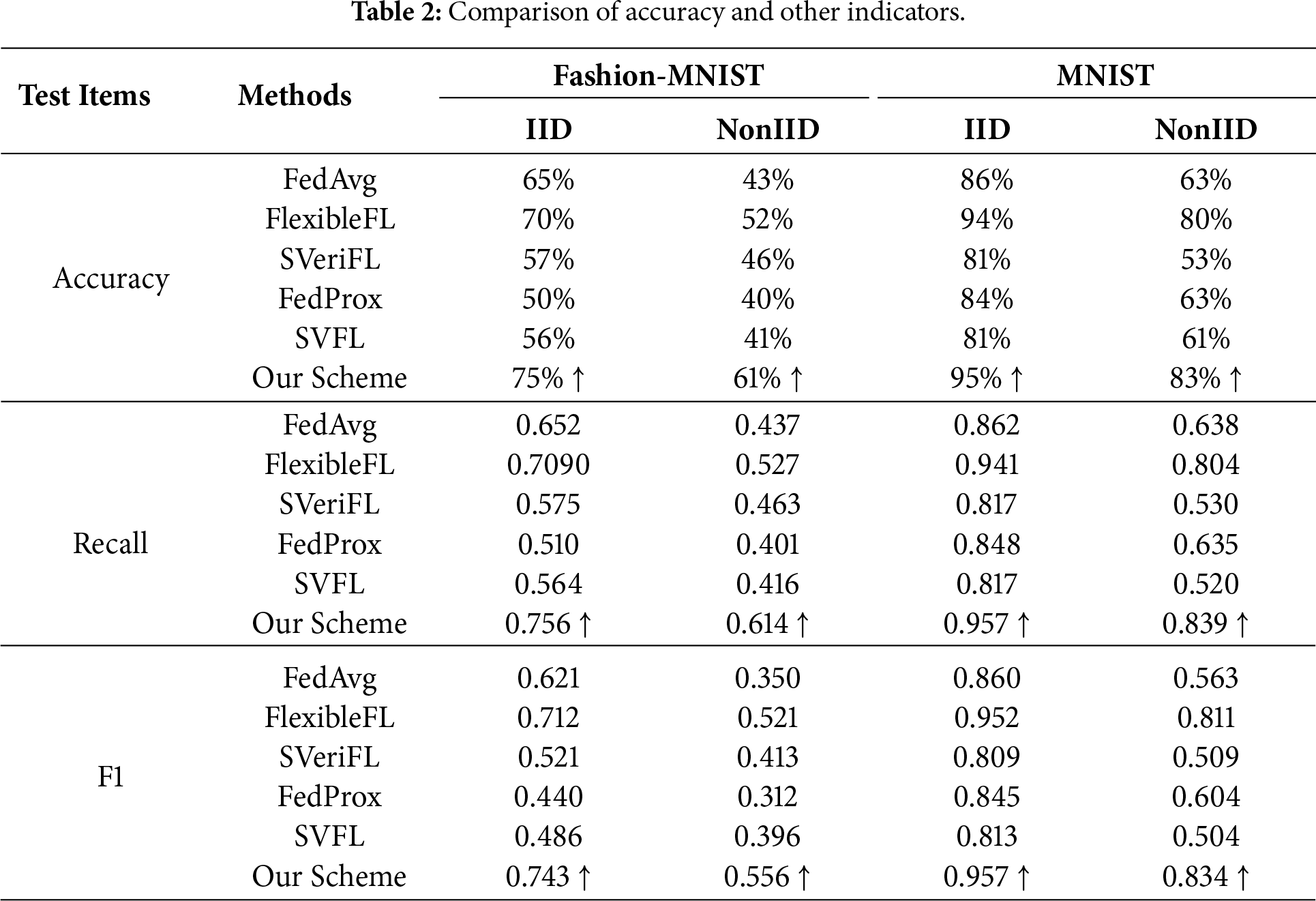
1) Accuracy comparative analysis in IID and Non-IID scenarios: In this experiment, we utilize two public available datasets to evaluate the performance of various federated learning schemes in two application scenarios. The accuracy of our scheme is compared with those of FedAvg [27], FlexibleFL [18], FedProx [28], SVeriFL [19], and SVFLC [20]. Table 2 presents the comparative results of test accuracy. In the IID scenario, our scheme achieves an accuracy exceeding 75% on the Fashion-MNIST dataset and approximately 95% on the MNIST dataset. In the Non-IID scenario, as the Non-IID setup simulates real-world conditions where users possess their own datasets, the training conditions for each user vary across rounds. As a result, the test accuracy curves exhibit greater fluctuations and converges more slowly. This behavior can be attributed to significant data heterogeneity across users, leading to inconsistent update directions for the local models. Consequently, the global model must adapt to these variations during aggregation, resulting in large fluctuations in test results and inconsistent accuracy across rounds. Despite the inconsistency in training effects due to varying datasets and models, our scheme demonstrates strong performance under both IID and Non-IID conditions. In terms of model accuracy comparison, we can see that our scheme is better than other schemes, which can prove that our scheme is effective in excluding malicious users.

2) Loss comparative analysis in IID and Non-IID scenarios: In this experiment, we compare the loss value of our scheme with the FedAvg, FlexibleFL, FedProx, SVeriFL and SVFLC. Fig. 4 presents the experimental results of the loss value variation. As shown in Fig. 4, our scheme exhibits significant advantages under the IID scenario. Specifically, after 100 training rounds, the loss value of our scheme on the MNIST dataset is reduced to 0.46, while on the FashionMNIST dataset it decreases to 0.83. These results indicate that our scheme not only effectively reduces the initial loss but also maintains a consistent downward trend throughout the training process. Notably, our scheme is the only one that exhibits a continuous decrease in loss value across all 100 epochs and reaches a desirable convergence state over a longer timescale. Furthermore, the overall experimental results show that, whether under IID or Non-IID conditions, our scheme consistently outperforms several other federated learning schemes. The non-IID configuration yields lower training loss, the corresponding test accuracy is lower than that of the IID setting. This indicates a potential mismatch between the training and testing distributions. Specifically, due to the skewed label distribution in non-IID data, users tend to overfit to a limited set of labels seen during training. As a result, the global model may fail to generalize to the full label space present in the test set, which contains uniformly distributed classes.

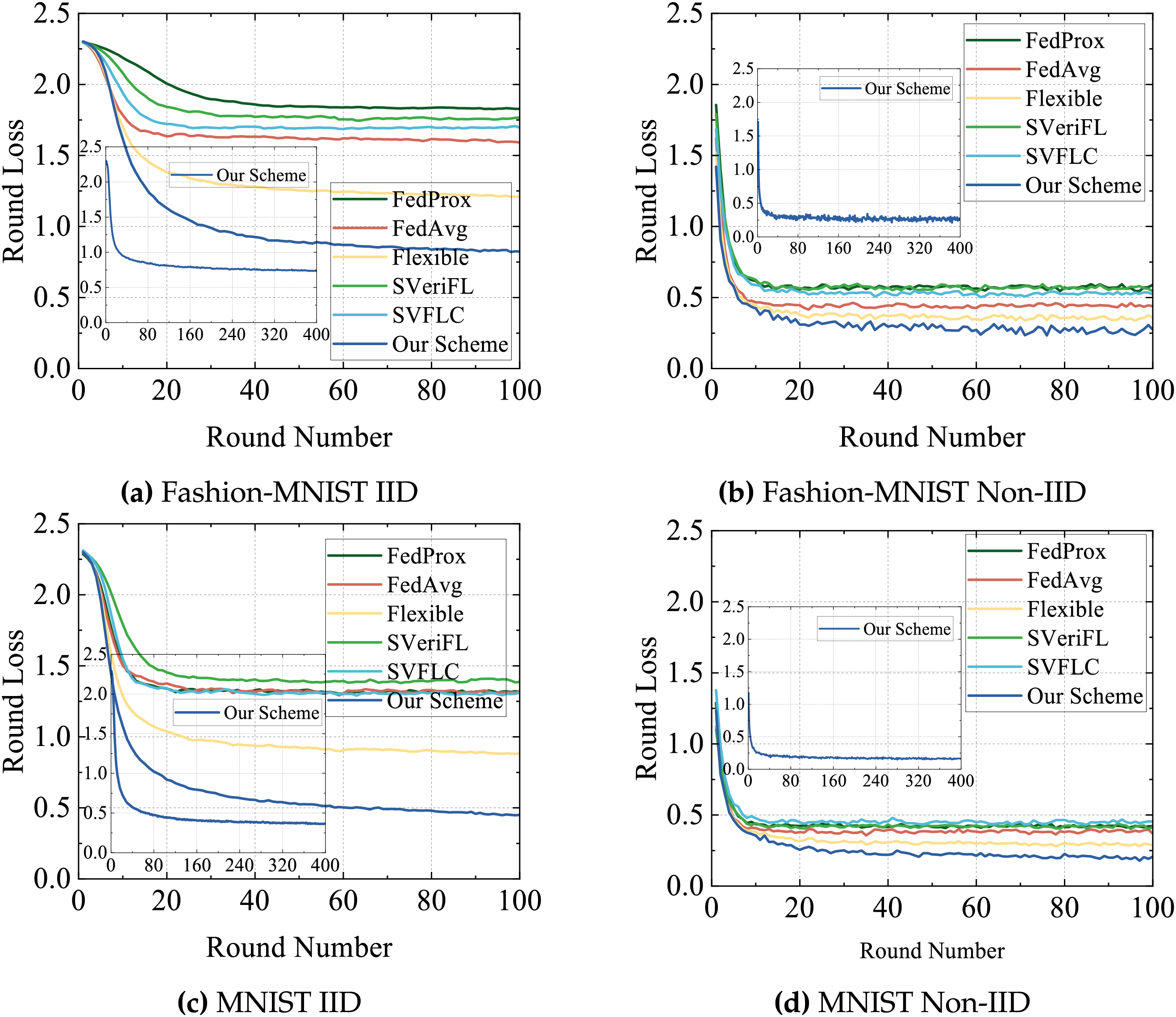
Figure 4: Comparison and analysis of loss on two datasets.

3) Training of other test indicators: We use a table to specifically show the final training of the above-mentioned indicators and some other indicators. Table 2 shows the comprehensive results for each indicator. From the table, it is evident that our scheme has good performance across all evaluation metrics, particularly in key indicators such as Recall Score and F1 Score, outperforming other existing schemes. These results demonstrate that our scheme not only enhances model accuracy but also maintains strong performance under complex data distribution conditions. Although the fluctuations occur in the Non-IID scenario for all schemes, our scheme consistently outperforms other schemes throughout the training process and in the final stage. This further validates the effectiveness of our scheme. Additionally, by filtering out some users who upload abnormal gradients during aggregation, our scheme can optimize both the model training speed and the final performance.

4) Performance comparison of different proportions of abnormal users: In this experiment, we compare the final model performance after 100 training rounds with 100 participants, varying the fraction of malicious users to 20%, 30%, and 40%. As shown in Figs. 5 and 6, with an increase in the number of abnormal users, all the schemes exhibit decreased test accuracy with slightly elevated final loss values. Notably, our scheme exhibits the least susceptibility to these adverse effects, underscoring its enhanced robustness in the exclusion of abnormal users. In contrast, other schemes suffer significant performance degradation due to their inability to effectively detect and manage anomalous user gradients. Benefiting from integrated anomaly detection mechanisms, our scheme is able to maintain superior performance metrics even as the proportion of anomalous users increases. Conversely, the performance of the other schemes regresses progressively, with the detrimental impact becoming increasingly severe as the proportion of abnormal users rises.

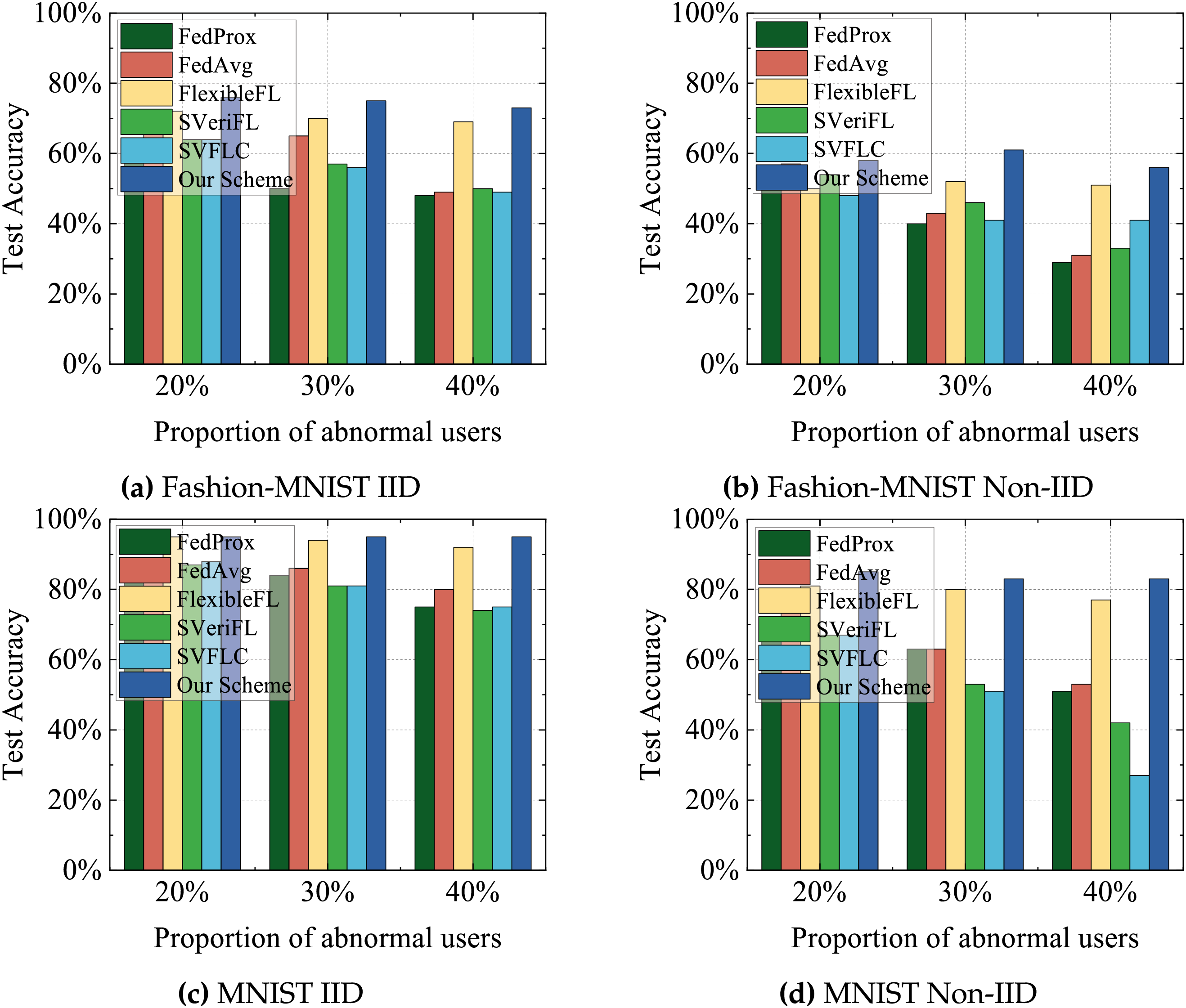
Figure 5: Comparison of accuracy under different proportions of abnormal users.

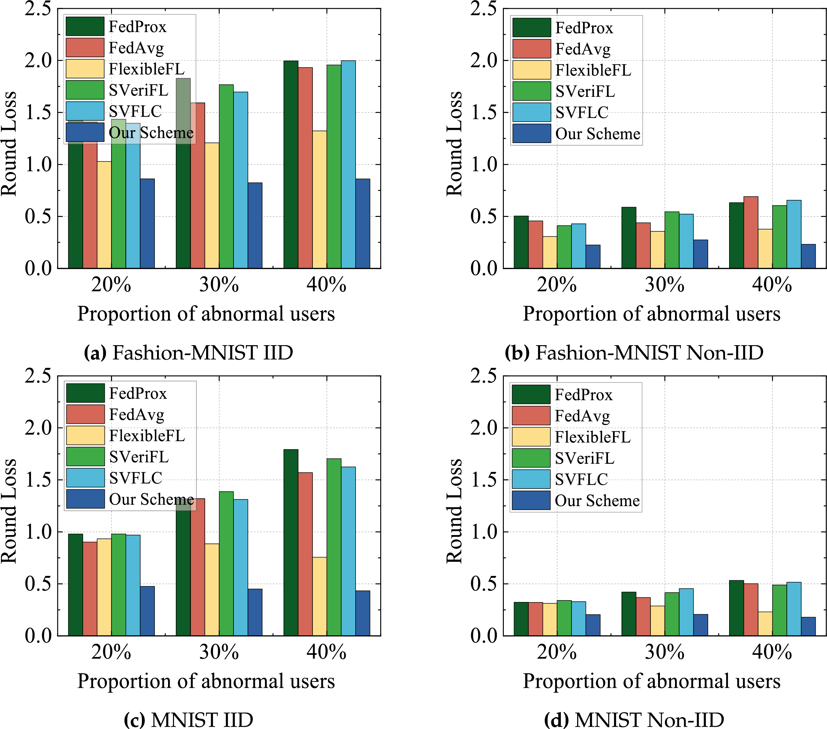
Figure 6: Comparison of loss under different proportions of abnormal users.

5) Compared with the free-riders detection schemes: In this experiment, we compare the final training results after 100 rounds of training with 100 users under different proportions of abnormal users, specifically with 20%, 30%, and 40% abnormal users. We compare the test accuracy and loss of our scheme with those of Krum [29], Median [30] in terms of robustness to aggregation accuracy. Fig. 7 shows the related experimental results. In the IID scenario, each user is assigned similarly distributed data, and the variance among benign updates remains relatively small. Under these homogeneous conditions, both Krum and Median achieve high accuracy when the proportion of abnormal users is low. This is because distance-based (Krum) and coordinate-wise (Median) aggregation methods can effectively identify and aggregate the majority of benign updates. However, as the proportion of abnormal users increases, Krum suffers from a sharp drop in accuracy and a noticeable increase in loss, reflecting reduced robustness. In contrast, our scheme consistently maintains high accuracy and stable loss. In the Non-IID scenario, users hold significantly different data distributions, resulting in greater variability among updates. Under such heterogeneous conditions, the performance of Krum and Median declines markedly. While accuracy declines and loss increases notably with a higher fraction of adversarial users, our scheme consistently achieves superior test accuracy and maintain low loss, highlighting its robustness and adaptability in varied environments.

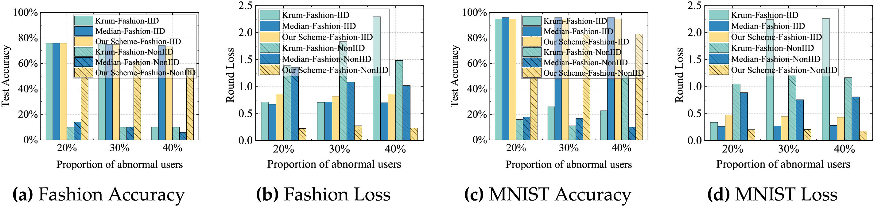
Figure 7: Comparison of test accuracy and loss among free-riders detection schemes across two datasets under both IID and Non-IID scenarios.

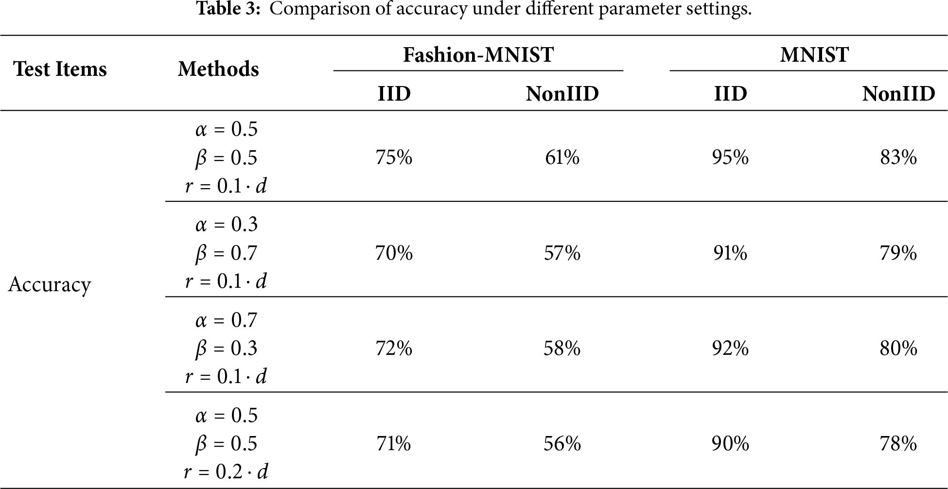
6) Ablation study results: The ablation results are shown in Table 3. The ablation experiments demonstrate that varying the weighting parameters α and β as well as the peer-sampling size r does not lead to substantial changes in performance; the resulting accuracy differences remain within a small range. This indicates that the proposed framework exhibits strong robustness and does not rely heavily on fine-grained parameter tuning. Moreover, under all tested configurations, the detection accuracy and loss convergence remain within normal statistical variation, confirming that the method maintains stable behavior across different parameter settings.

7) Evaluation under label-flipping poisoning attacks: To examine whether the proposed CF-JL verification can distinguish poisoned updates from benign non-IID behavior, we further evaluate the system under the label-flipping attack, where malicious users invert labels during training. We compare our scheme with Median and Krum, two widely used Byzantine-robust aggregation baselines. The results show that all three methods are able to suppress the degradation caused by poisoned users. Our scheme achieves detection accuracy and global-model robustness comparable to these baselines. This indicates that the gradient-feature representation used in the collaborative-filtering verification still captures structural inconsistencies induced by poisoning, even when the attack is embedded in a seemingly “honest” training process. These findings also confirm that our approach can function as an effective verification component for mitigating harmful updates and can be combined with robust aggregation algorithms to further strengthen FL security under stronger poisoning threat models, as illustrated in Fig. 8.

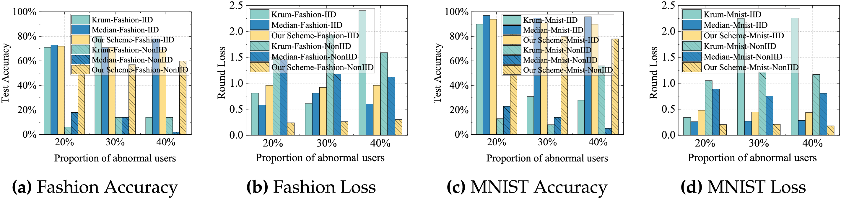
Figure 8: Comparison of test accuracy and loss among poisoning detection schemes across two datasets under both IID and Non-IID scenarios.

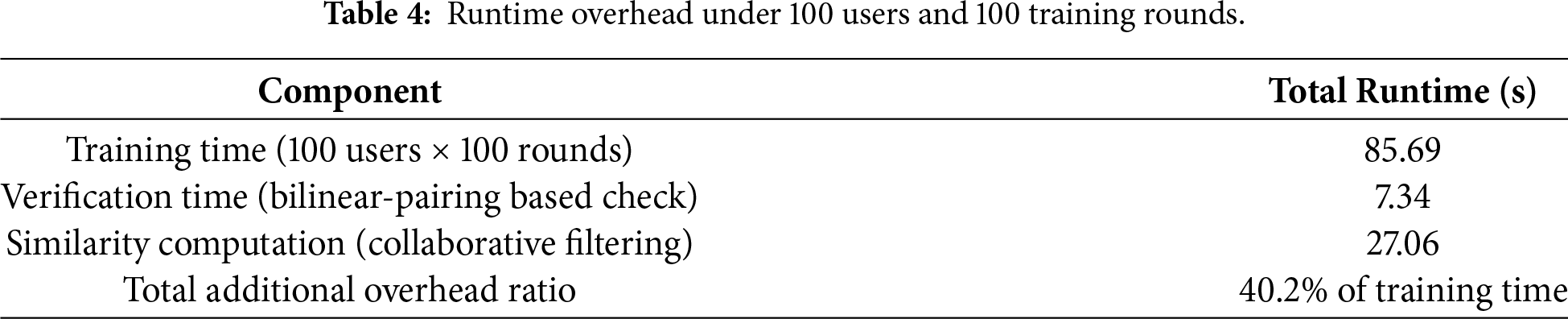
8) Runtime and complexity analysis: The verification overhead remains small relative to the overall training time. As shown in Table 4, under 100 users and 100 training rounds, the combined cost of verification and similarity analysis accounts for only a minor portion of the total runtime, indicating that the proposed scheme is efficient and adds only limited latency. The results confirm that the collaborative-filtering-based verification remains time-effective and scales well with the number of users.

5  Future Work

Several promising directions remain for future investigation. While this paper focuses on representative free-riding behaviors and label-flipping poisoning attacks, the emergence of more sophisticated adaptive adversaries deserves further attention. In particular, attackers that deliberately mimic benign clients pose a greater challenge to existing similarity-based verification mechanisms. Extending the proposed framework to address such adaptive threats by incorporating richer temporal constraints or cross-round behavioral consistency analysis is a priority for our future research. And the present evaluation primarily considers CNN-based image classification tasks on MNIST and Fashion-MNIST. Although the proposed verification mechanism is model-agnostic and operates on gradient-level representations, further validation on larger-scale datasets (e.g., CIFAR-10/100), deeper models, and non-vision modalities such as text classification would provide a more comprehensive assessment of its scalability and generality. Investigating the performance-efficiency trade-offs in these complex settings remains a critical objective for future work.

6  Conclusion

In this paper, we propose a gradient feature-based collaborative filtering scheme in verification federated learning, where the authenticity of user training is verified using the CF method based on gradient features and user gradient security is protected by dynamically generating a mask matrix. Further, to show the effectiveness of our scheme, we conduct an in-depth security analysis to demonstrate its resilience against some malicious attacks. Subsequently, we assess its practicality by comparing its performance with several state-of-the-art schemes on the MNIST and Fashion-MNIST datasets.

Acknowledgement: Not applicable.

Funding Statement: This work was supported by the National Natural Science Foundation of China (No. 62572077), Open Research Fund of Hunan Provincial Key Laboratory of Intelligent Processing of Big Data on Transportation (No. B202403), and Hunan Provincial Social Science Achievement Evaluation Committee (No. XSP25YBC686).

Author Contributions: The authors confirm contribution to the paper as follows: Study conception and design: Chen Yu, Ke Gu; data collection: Chen Yu; analysis and interpretation of results: Chen Yu, Ke Gu, Jingjing Tan; draft manuscript preparation: Chen Yu, Ke Gu, Wenwu Zhao. All authors reviewed and approved the final version of the manuscript.

Availability of Data and Materials: The datasets used in this paper are respectively in references [25,26].

Ethics Approval: Not applicable.

Conflicts of Interest: The authors declare no conflicts of interest.

References

1. Zhu L, Han S. Deep leakage from gradients. In: Federated learning: Privacy and incentive. Cham, Switzerland: Springer; 2020. p. 17–31. doi:10.1007/978-3-030-63076-8_2. [Google Scholar] [CrossRef]

2. Shokri R, Stronati M, Song C, Shmatikov V. Membership inference attacks against machine learning models. In: 2017 IEEE Symposium on Security and Privacy (SP). Piscataway, NJ, USA: IEEE; 2017. p. 3–18. [Google Scholar]

3. Wang Z, Huang Y, Song M, Wu L, Xue F, Ren K. Poisoning-assisted property inference attack against federated learning. IEEE Trans Dependable Secure Comput. 2023;20(4):3328–40. doi:10.1109/tdsc.2022.3196646. [Google Scholar] [CrossRef]

4. Sun L, Lyu L. Federated model distillation with noise-free differential privacy. arXiv:2009.05537. 2020. [Google Scholar]

5. Wei K, Li J, Ding M, Ma C, Yang HH, Farokhi F, et al. Federated learning with differential privacy: algorithms and performance analysis. IEEE Trans Inf Forensics Secur. 2020;15:3454–69. [Google Scholar]

6. Phong LT, Aono Y, Hayashi T, Wang L, Moriai S. Privacy-preserving deep learning via additively homomorphic encryption. IEEE Trans Inf Forensics Secur. 2018;13(5):1333–45. doi:10.1109/tifs.2017.2787987. [Google Scholar] [CrossRef]

7. Fraboni Y, Vidal R, Lorenzi M. Free-rider attacks on model aggregation in federated learning. In: International Conference on Artificial Intelligence and Statistics. London, UK: PMLR; 2021. p. 1846–54. [Google Scholar]

8. Lin J, Du M, Liu J. Free-riders in federated learning: attacks and defenses. arXiv:1911.12560. 2019. [Google Scholar]

9. Fang M, Cao X, Jia J, Gong N. Local model poisoning attacks to byzantine-robust federated learning. In: 29th USENIX Security Symposium (USENIX Security 20); 2020 Aug 12–14; Boston, MA, USA. p. 1605–22. [Google Scholar]

10. Zhang J, Chen B, Cheng X, Binh HTT, Yu S. PoisonGAN: Generative poisoning attacks against federated learning in edge computing systems. IEEE Internet Things J. 2021;8(5):3310–22. doi:10.1109/jiot.2020.3023126. [Google Scholar] [CrossRef]

11. Xu G, Li H, Liu S, Yang K, Lin X. VerifyNet: secure and verifiable federated learning. IEEE Trans InfForensics Secur. 2020;15:911–26. [Google Scholar]

12. Wang G, Zhou L, Li Q, Yan X, Liu X, Wu Y. FVFL: a flexible and verifiable privacy-preserving federated learning scheme. IEEE Internet Things J. 2024;11(13):23268–81. [Google Scholar]

13. Fu A, Zhang X, Xiong N, Gao Y, Wang H, Zhang J. VFL: a verifiable federated learning with privacy-preserving for big data in industrial IoT. IEEE Trans Ind Inform. 2022;18(5):3316–26. [Google Scholar]

14. Xia Y, Liu Y, Dong S, Li M, Guo C. SVCA: secure and verifiable chained aggregation for privacy-preserving federated learning. IEEE Internet Things J. 2024;11(10):18351–65. [Google Scholar]

15. Guo X, Liu Z, Li J, Gao J, Hou B, Dong C, et al. VeriFL: communication-efficient and fast verifiable aggregation for federated learning. IEEE Trans Inf Forensics Secur. 2021;16:1736–51. [Google Scholar]

16. Wang H, Guo Y, Bie R, Jia X. Verifiable arbitrary queries with zero knowledge confidentiality in decentralized storage. IEEE Trans Inf Forensics Secur. 2024;19:1071–85. doi:10.1109/tifs.2023.3330305. [Google Scholar] [CrossRef]

17. Du R, Li X, He D, Choo KKR. Toward secure and verifiable hybrid federated learning. IEEE Trans Inf Forensics Secur. 2024;19:2935–50. doi:10.1109/tifs.2024.3357288. [Google Scholar] [CrossRef]

18. Zhao Y, Cao Y, Zhang J, Huang H, Liu Y. FlexibleFL: mitigating poisoning attacks with contributions in cloud-edge federated learning systems. Inf Sci. 2024;664:120350. [Google Scholar]

19. Gao H, He N, Gao T. SVeriFL: successive verifiable federated learning with privacy-preserving. Inf Sci. 2022;622:98–114. [Google Scholar]

20. Li N, Zhou M, Yu H, Chen Y, Yang Z. SVFLC: secure and verifiable federated learning with chain aggregation. IEEE Internet Things J. 2024;11(8):13125–36. [Google Scholar]

21. Ammad-ud-din M, Ivannikova E, Khan SA, Oyomno W, Fu Q, Tan KE, et al. Federated rollaborative filtering for privacy-preserving personalized recommendation system. arXiv:1901.09888. 2019. [Google Scholar]

22. Perifanis V, Efraimidis PS. Federated neural collaborative filtering. Knowl Based Syst. 2022;242:108441. doi:10.1016/j.knosys.2022.108441. [Google Scholar] [CrossRef]

23. Gao S, Luo J, Zhu J, Dong X, Shi W. VCD-FL: verifiable, collusion-resistant, and dynamic federated learning. IEEE Trans Inf Forensics Secur. 2023;18:3760–73. [Google Scholar]

24. Johnson WB, Lindenstrauss J. Extensions of Lipschitz mappings into Hilbert space. Contemp Math. 1984;26:189–206. doi:10.1090/conm/026/737400. [Google Scholar] [CrossRef]

25. LeCun Y, Cortes C. The mnist database of handwritten digits; 2005 [cited 2025 Dec 15]. Available from: https://api.semanticscholar.org/CorpusID:60282629. [Google Scholar]

26. Xiao H, Rasul K, Vollgraf R. Fashion-MNIST: a novel image dataset for benchmarking machine learning algorithms. arXiv:1708.07747. 2017. [Google Scholar]

27. McMahan B, Moore E, Ramage D, Hampson S, Arcas BAY. Communication-efficient learning of deep networks from decentralized data. In: Proceedings of the 20th International Conference on Artificial Intelligence and Statistics (AISTATS) 2017; 2017 Apr 20–22; Fort Lauderdale, FL, USA. 2017. p. 1273–82. [Google Scholar]

28. Li T, Sahu AK, Zaheer M, Sanjabi M, Talwalkar A, Smith V. Federated optimization in heterogeneous networks. Proc Mach Learn Syst. 2020;2:429–50. [Google Scholar]

29. Blanchard P, El Mhamdi EM, Guerraoui R, Stainer J. Machine learning with adversaries: byzantine tolerant gradient descent. In: Guyon I, Luxburg UV, Bengio S, Wallach H, Fergus R, Vishwanathan S et al., editors. Advances in neural information processing systems. Vol. 30. Red Hook, NY, USA: Curran Associates, Inc.; 2017. p. 1–11. [Google Scholar]

30. Yin D, Chen Y, Kannan R, Bartlett P. Byzantine-robust distributed learning: towards optimal statistical rates. In: Dy J, Krause A, editors. Proceedings of the 35th International Conference on Machine Learning. Vol. 80. London, UK: PMLR; 2018. p. 5650–9. [Google Scholar]