BCAM-Net: A Bidirectional Cross-Attention Multimodal Network for IoT Spectrum Sensing under Generalized Gaussian Noise

1  Introduction

The rise of the information and digital era has opened unprecedented opportunities for wireless communications. As a key technology connecting the physical and digital worlds, the internet of things (IoT) is experiencing explosive growth [1]. This growth spans many critical domains, such as the industrial internet of things(IIoT) [2], smart grid [3], and vehicle-to-everything (V2X) systems [4], and drives demand for access by massive heterogeneous devices. With the concurrent access of a large number of devices, the finite wireless spectrum is under unprecedented pressure, since the available bands are limited while the number of accessing devices and their data demands continue to increase [5]. The traditional fixed spectrum allocation mechanism, which assigns specific bands exclusively and long-term to primary users (PUs), struggles to meet such dynamic and diverse access needs, resulting in low spectrum utilization and further intensifying spectrum scarcity [6].

To address spectrum scarcity, cognitive radio (CR) is regarded as a highly promising solution [7]. In IoT networks, CR allows secondary users (SUs)—such as wireless sensor nodes and industrial controllers in the IIoT, environmental monitoring devices and intelligent street-light systems in smart cities, and on-board units (OBUs) and roadside units (RSUs) in V2X systems—to dynamically access temporarily idle licensed bands that are not occupied by PUs, thereby improving spectrum utilization efficiency [8]. As the first critical step of CR, the accuracy of spectrum sensing directly affects the system’s understanding of spectrum occupancy and the rationality of subsequent decisions [9]. Efficient spectrum sensing enables SUs to accurately detect idle spectrum, avoid collisions with spectrum occupied by PUs and protect PU communication quality, while also optimizing communication performance and improving spectrum utilization. Therefore, spectrum sensing is fundamental to the efficient operation of CR systems, and the study of reliable and efficient spectrum sensing techniques is particularly important.

Traditional spectrum sensing techniques are mostly based on energy detection and correlation analysis, and are simple and easy to implement [10]. However, their adaptability to complex electromagnetic environments is limited, and they exhibit poor performance, especially under low signal-to-noise ratios (SNRs) and weak-signal conditions [11]. Meanwhile, traditional methods often model the disturbance as additive white Gaussian noise (AWGN), which is reasonable for thermal-noise-limited cellular or laboratory environments. In many practical IoT-oriented wireless scenarios, however, this assumption no longer holds: non-Gaussian noise (such as atmospheric noise and man-made electromagnetic interference) becomes dominant [12]. As shown in Fig. 1, such noise sources are widespread in typical IoT scenarios including the IIoT and V2X, for example industrial motors, vehicle ignition, and power-grid transients. This type of noise exhibits impulsive peaks and long tails and is one of the main sources of errors in wireless systems [13]; therefore, achieving highly robust spectrum sensing under non-Gaussian conditions is a key challenge in IIoT scenarios.

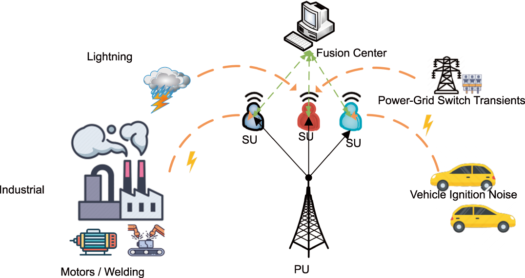
Figure 1: Non-Gaussian noise and cooperative spectrum sensing in IoT.

Since the essence of spectrum sensing is a binary classification problem that decides whether a signal is present [14], machine learning (ML) and deep learning (DL) offer new approaches to address the limitations of traditional methods under low SNR and non-Gaussian noise. With strong nonlinear modeling and data-driven feature extraction capabilities [15,16], ML/DL can reduce the strict reliance on prior signal information and instead learn subtle differences between signal and noise directly from the data.

Early studies mainly focused on traditional ML methods [17,18]. Saber et al. used the received signal energy as a feature, trained and tested artificial neural networks (ANNs) and support vector machine (SVM) classifiers to categorize received data as PU signal or noise, and concluded that SVM-based spectrum sensing was more accurate than ANN-based classification [19]. Varma and Mitra proposed a blind sensing model based on SVM, trained with two statistical features—smoothed correlation of reversed spectrum segments (SCRSS) and variance of multi-scale moving averages (VMMA)—which effectively detected spectrum signals at an SNR of −13 dB [20]. Saravanan et al. addressed spectrum sensing under generalized Gaussian (non-Gaussian) noise by using differential entropy (DE) estimates as features combined with supervised classifiers such as SVM, k-nearest neighbors (KNN), and random forest; the method effectively distinguished noise from signal at low SNRs and under heavy-tailed noise, outperforming traditional energy detection [21]. However, these traditional machine learning methods rely heavily on handcrafted feature extraction; the quality of such features directly determines the performance ceiling of the models and leads to limited robustness.

In recent years, DL with stronger end-to-end learning capabilities has been widely applied in wireless communications, providing new approaches to spectrum sensing [22,23]. Chen et al. proposed a spectrum sensing method based on the short-time Fourier transform (STFT) and a convolutional neural network (CNN) [24]. The method extracts time-frequency information using STFT and then performs classification with a CNN. To better capture the time-frequency characteristics of wireless signals, several studies employ the continuous wavelet transform (CWT) to convert IQ samples into time-frequency images as inputs to deep learning models. Zhen et al. addressed spectrum sensing of nonstationary signals under low SNRs by combining CWT with a residual network (ResNet) [25]. Their method first converts the signal into a time-frequency matrix via CWT and then feeds it into a ResNet classifier. The approach is fully data-driven and does not require prior information, and their results indicate that the Morlet wavelet yields the best detection performance among the tested options. Xu et al. transformed the IQ signals collected by secondary users into CWT-based time-frequency images and fed them into a Swin-Transformer for spectrum sensing [26]. Experimental results show that, compared with conventional CNN-based methods, this approach achieves significantly better detection performance at low SNRs, further confirming the effectiveness of CWT as a feature extractor for spectrum sensing. To improve spectrum utilization and minimize interference, Varma et al. employed CWT to transform the IQ signals of multiple wireless technologies into time-frequency images and, based on these representations, designed a lightweight CNN for signal identification [27]. Their method achieves over 90% classification accuracy, indirectly confirming the effectiveness of CWT for wireless signal feature extraction and providing valuable insights for spectrum sensing in complex coexistence environments. These CWT-based approaches demonstrate that time-frequency representations are highly informative for spectrum sensing. However, they typically treat the CWT image as a single modality and rarely explore explicit interactions with temporal features. Fang et al. proposed a CNN-Transformer hybrid model to address the inability of DL-based cooperative spectrum sensing (CSS) to extract correlations across different SUs [28]. The model exploits temporal correlations within each SU and features across SUs, and also considers imperfect reporting channels. Simulations show superior performance, with about a 6 dB improvement over traditional energy detection; however, the CNN-Transformer hybrid architecture results in relatively high model complexity. To utilize both sequence information and time-frequency information, some studies have proposed more complex hybrid models. Gao et al. proposed a GAN-GRU-YOLO model for consumer IoT scenarios [29]. The method builds a dual-branch network: it uses the continuous wavelet transform (CWT) to obtain a spectrogram and employs YOLOv5 to capture higher-order time-frequency information, and it combines GRU and CNN branches to extract features from the raw time series. Generative adversarial networks (GANs) are also used for data augmentation. The method achieves high detection probability, but performance degrades markedly at low SNRs. Recently, attention mechanisms and Transformer architectures have been introduced into spectrum sensing. Zhang et al. proposed Spectrum Transformer, a multi-head self-attention-based wideband spectrum detector that operates on PSD data to jointly learn intra-band spectral features and long-range inter-band dependencies, and employs a multi-task output structure for multi-band occupancy detection, thereby highlighting the advantage of attention mechanisms in wideband spectrum sensing [30]. Xi et al. proposed a time-frequency cross-fusion network (TFCFN) to improve sensing performance under generalized Gaussian distribution (GGD) noise [31]. The model adopts a dual-branch architecture: one branch uses GRU to capture temporal dependencies from the raw signal, and the other performs FFT followed by a CNN to extract frequency-domain features, with the two streams fused via a cross-attention mechanism. While TFCFN demonstrates the effectiveness of cross-modal fusion under the GGD noise model, its cross-attention fusion is typically implemented in a single-direction manner, leading to an asymmetric interaction where one stream is conditioned on the other. Under impulsive non-Gaussian noise, modality-specific distortions may occur in either the time-frequency or temporal stream; therefore, a one-way interaction may be insufficient to ensure robust and stable performance, especially in the low-SNR regime. Beyond spectrum sensing, cross-attention and bidirectional cross-attention have also been explored for feature fusion in other signal-related tasks (e.g., radio frequency interference identification using dual cross-attention and multi-scale feature fusion [32] and time-frequency fusion using bidirectional cross-attention to allocate weights for robust diagnosis under interference [33]), where two-way interactions can facilitate mutual refinement between heterogeneous representations and may help alleviate representation-specific noise. These findings motivate exploring whether explicitly modeling two-way interactions can help improve fusion stability under impulsive GGD noise, particularly in the low-SNR regime. To the best of our knowledge, these studies have not explicitly investigated such bidirectional interaction in the context of spectrum sensing under impulsive non-Gaussian noise.

Accordingly, to improve the stability and robustness of spectrum sensing in complex IoT scenarios under impulsive GGD noise, this paper proposes a bidirectional cross-attention multimodal network (BCAM-Net). The key idea of BCAM-Net lies in its bidirectional cross-attention fusion, which allows the model to adaptively cross-enhance temporal and time-frequency features under uncertain noise conditions. Compared with one-directional fusion, the bidirectional design mitigates the risk that modality-specific distortions in either stream dominate the fusion, thereby helping stabilize the fused representation even when one stream is heavily corrupted.

The main contributions are as follows:

•   Construction of multimodal inputs for GGD noise and low SNR scenarios:

         Time-frequency path: for each SU, the received complex IQ sequence is processed by continuous wavelet transform (CWT) to form an I/Q two-channel time-frequency tensor, which is stacked along the SU dimension to capture local time-frequency textures and global energy distribution. Unlike existing works, the aggregation of per-SU CWT features across the SU dimension explicitly exploits spatial diversity across SUs, improving robustness to impulsive and bursty GGD noise;

         Temporal path: in the complex domain, cooperative averaging is performed over multiple SU signals to extract magnitude and phase sequences, which characterize the temporal evolution of the envelope and phase. This cooperative temporal representation suppresses SU-specific impulsive outliers, yielding a more stable temporal signature under heavy-tailed noise.

•   Bidirectional cross-attention (BCA) module for cross-modal consistency correction, designed with two paths for spectrum sensing under non-Gaussian noise:

         Temporal → time-Frequency: temporal features guide the time-frequency branch to focus on discriminative regions consistent with temporal evolution, thereby mitigating spurious peaks and textures in the time-frequency map;

         Time-Frequency → Temporal: global time-frequency features guide the verification of each time step in the temporal sequence, suppressing short-term abnormal fluctuations induced by GGD noise. In contrast to existing one-directional fusion architectures (e.g., TFCFN) or cascaded CNN-Transformer models, the proposed BCA design enables bidirectional calibration between modalities, thereby maintaining high detection performance and robustness even under GGD noise with varying shape parameters.

•   Simulation results verify the superiority and robustness of the proposed BCAM-Net. The results show that, in the low-SNR region, BCAM-Net achieves better detection performance than multiple baseline methods; for example, at SNR −14 dB and false alarm probability Pf=0.1, it attains a detection probability of 0.9020. Moreover, BCAM-Net maintains high detection performance under various GGD shape parameters. For instance, when the SNR is −10 dB and Pf=0.1, the detection probability of BCAM-Net remains above 0.90 when it is trained, validated, and tested separately on datasets generated under each fixed GGD shape parameter β∈{0.3,0.5,0.6,1.0,1.6,2.0}. Compared with spectrum sensing methods that can achieve high detection probability only under a specific shape parameter (e.g., β=0.5), BCAM-Net exhibits much better robustness.

The remainder of this paper is organized as follows. Section 2 describes the system model. Section 3 presents the multimodal spectrum sensing model for GGD noise. Section 4 provides the experiments and performance evaluation. Section 5 concludes the paper.

2  System Model

The multiuser cooperative spectrum sensing model considered in this study is illustrated in Fig. 2. Each SU independently samples the signal from the PU. The extracted data are then transmitted to the fusion center via a reporting channel, where a soft-fusion decision is performed; the final decision is subsequently fedback to the SUs.

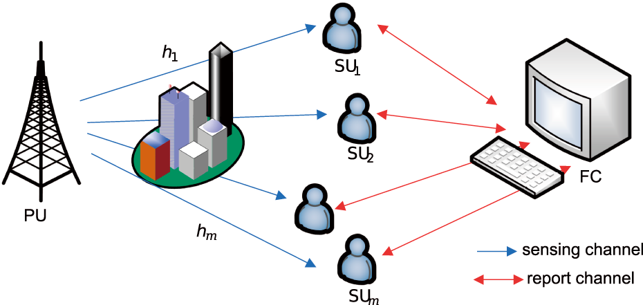
Figure 2: Cooperative spectrum sensing model.

The cooperative spectrum sensing model consists of a single-antenna Primary User (PU) and multiple Secondary Users (SUs). The SUs sense whether the PU is active. Under a binary hypothesis test, the signal received by the m-th SU can be expressed as:

xm(n)={wm(n),H0,n=1,2,…,N,hm(n)s(n)+wm(n),H1,n=1,2,…,N,(1)

where there are two hypotheses H0 and H1. Under H0, the channel contains only noise samples wm(n); the PU signal s(n) is absent and the channel can be used by SUs. Under H1, both noise and the PU signal s(n) are present and the channel cannot be used. Here m=1,2,…,M, where M denotes the number of SUs; hm(n) is the complex channel gain between the m-th SU and the PU and is modeled as a zero-mean circularly symmetric complex Gaussian random variable with unit variance, i.e., hm(n)∼𝒞𝒩(0,1), so that |hm(n)| follows a Rayleigh distribution with unit average power. N denotes the number of observed samples.

The sensing performance of spectrum sensing algorithms is usually evaluated by the false-alarm probability Pf and the detection probability Pd [34]. The false alarm probability Pf is defined as the probability of declaring the PU present when it is actually absent:

{Pf=Pr{H1∣H0},Pd=Pr{H1∣H1},(2)

where Pd denotes the detection probability, i.e., the probability of correctly declaring the PU present when it is present.

To more accurately characterize the impulsive non-Gaussian noise that SUs may encounter from sources such as industrial motors, electric welding and vehicle ignition systems, this paper adopts the Generalized Gaussian Distribution GGD to describe the statistics of the noise wm(n). In this cooperative sensing model, accurate spectrum sensing becomes more challenging in the presence of such non-Gaussian impulsive noise, which motivates us to consider a more robust sensing model. The GGD can depict various types of heavy-tailed impulsive noise by adjusting its parameters [35]. The probability density function is

fX(wm(n))=12αΓ(1β)exp(−|wm(n)|βα),wm(n)∈R,(3)

where α>0 controls the scale of the density function and 0<β≤2 is the shape parameter. As illustrated in Fig. 3, a smaller β produces a sharper peak and heavier tails, indicating stronger impulsive noise; as β increases, the peak becomes lower and the tails become lighter, gradually approaching the Gaussian case and thus weakening the non-Gaussian property.

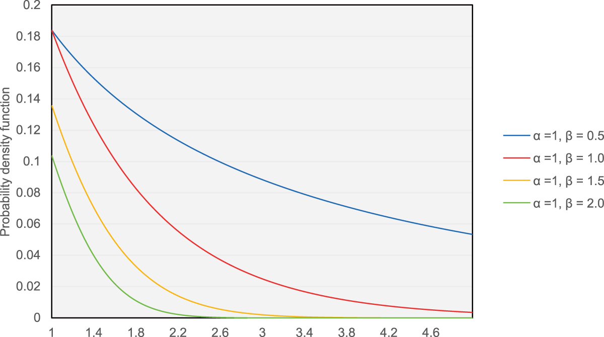
Figure 3: Probability density function of GGD distribution under different shape parameters.

In our simulations, α is fixed to 1 to generate a unit-scale noise prototype, and the target SNR is controlled by power normalization (i.e., rescaling the generated noise to match the desired noise power). Therefore, α=1 is without loss of generality, while β is used to vary the impulsiveness of the noise in the robustness tests.

3  Multimodal Spectrum Sensing Model for GGD Noise

To achieve stable spectrum sensing in complex IoT scenarios, we propose a bidirectional cross-attention multimodal network (BCAM-Net) for spectrum sensing under GGD noise (see Fig. 4). The model exploits two complementary modalities: (i) time-frequency images of multiple SUs (obtained by applying CWT to the I/Q components) and (ii) magnitude-phase features of the cooperative IQ sequence. Feature representations are extracted by a time-frequency branch and a temporal branch, respectively. BCA is then introduced to guide the time-frequency branch with temporal information and to constrain the temporal representation with time-frequency information, enabling cross-modal complementarity and improved robustness when heavy-tailed noise coexists with weak signals. Finally, the model fuses three vectors—the original global time-frequency vector, the temporally guided time-frequency vector, and the temporal vector guided by time-frequency features—and outputs a binary decision.

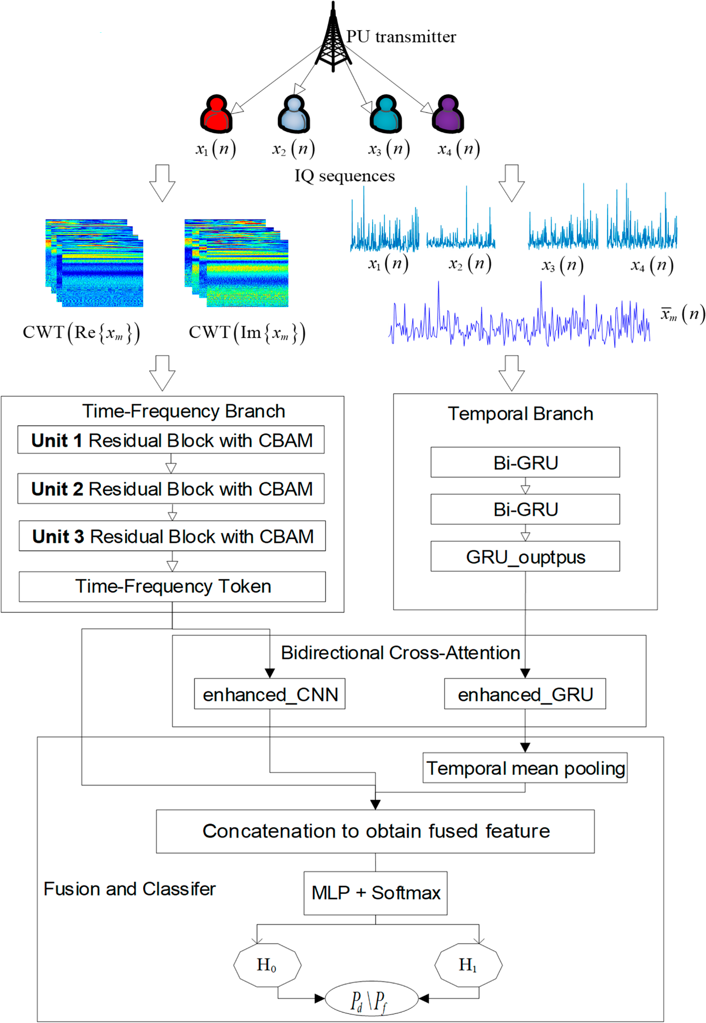
Figure 4: BCAM-Net model diagram.

3.1 Data and Input Construction

To preserve spatial diversity across SU receivers, the CWT is computed independently for the complex IQ sequence of the m-th SU, xm(n), yielding the complex coefficient matrix CWT(xm). In continuous time, the CWT of a signal x(t) is defined as

W(a,b)=1|a|∫−∞+∞x(t)ψ∗(t−ba)dt,(4)

where W(a,b) denotes the CWT coefficient of x(t) at scale a>0 and translation b, ψ(⋅) the mother wavelet, and (⋅)∗ the complex conjugate.

Complex Morlet wavelet is adopted, owing to its favorable time-frequency localization and approximate analyticity, which preserves phase information while producing smooth time-frequency textures—properties particularly effective for discriminating signal from noise in spectrum-sensing tasks [25]. The complex Morlet analyzing wavelet is defined as

ψ(t)=π−1/4exp⁡(j2πt⋅1)exp⁡(−t2100).(5)

For the m-th SU, the CWT of the complex IQ sequence xm(n) yields a complex coefficient matrix Wxm∈CH×W, where H and W denote the numbers of discrete scales and time positions (translations), respectively. The real and imaginary parts are stacked along the channel axis to obtain

Cm=[Re⁡{Wxm},Im⁡{Wxm}]∈R2×H×W.(6)

For implementation, we compute the discrete CWT using the complex Morlet wavelet with sampling frequency fs=200 kHz (Δt=1/fs). The translation is sampled at all time indices within each sensing window, i.e., b∈{0,1,…,N−1}, hence W = N (with N=256 in our dataset). To discretize the scale, we first define a frequency grid {fi}i=1H over [fmin,fmax] with fmax=fs/2 and fmin=fs/(2H), and use a log-spaced sampling. The corresponding scales are computed as

ai=fcfiΔt,i=1,…,H,(7)

where fc is the wavelet-dependent center frequency. In this work, we set H=128, yielding a CWT matrix of size H×W=128×256 for each SU.

Stacking {Cm}m=1M along the SU dimension produces the time-frequency input tensor for the CNN branch:

ximg=stack⁡(C1,…,CM)∈RM×2×H×W,(8)

where M is the number of SUs, the second dimension corresponds to the real and imaginary channels, and (H,W) represent the scale and time dimensions of the CWT, respectively.

For the temporal branch, cooperative IQ magnitude-phase features are employed to capture robust temporal statistics and phase dynamics. Complex observations from M SUs, {xm(n)}m=1M, are averaged in the complex domain as

x¯(n)=1M∑m=1Mxm(n),(9)

which serves as the complex-valued input sequence for the temporal branch. Each complex sample x¯(n) is converted into a two-dimensional real-valued feature vector

xn=[|x¯(n)|RMS∠x¯(n)]∈R2,(10)

where |x¯(n)|RMS denotes the RMS-normalized magnitude and ∠x¯(n) denotes the phase.

3.2 Time-Frequency Branch

To achieve stable spectrum sensing under GGD noise, the time-frequency branch takes as input the SU-stacked time-frequency tensor

ximg={Cm}m=1M,Cm∈R2×H×W,(11)

where, Cm is formed by stacking the real and imaginary parts of the complex CWT coefficients of the m-th SU along the channel dimension. The objective of this branch is to extract discriminative global representations from the 2D time-frequency plane that indicate PU occupancy. To this end, the branch adopts a residual convolutional stack with CBAM attention, global pooling, and SU-wise averaging. The front end uses three attention-augmented residual blocks to suppress irrelevant channels and spatial regions while highlighting discriminative spectral-temporal textures, whereas the back end applies adaptive global average pooling to obtain a vector for each SU and then performs SU-wise arithmetic averaging to produce the global time-frequency vector, which serves as the input to the subsequent BCA attention and fusion classifier.

3.2.1 Residual Block with Convolutional Block Attention Module

The fusion unit of the residual block and the Convolutional Block Attention Module (CBAM) is illustrated in Fig. 5. The unit consists of convolution (Conv), batch normalization (BN), CBAM attention, residual addition and Rectified Linear Unit (ReLU). Convolution extracts locally correlated features within the time-frequency neighborhood; BN stabilizes feature statistics and accelerates convergence; CBAM re-calibrates features through channel-wise and spatial attention in sequence to highlight discriminative responses; residual addition provides a direct gradient pathway to alleviate degradation, and ReLU supplies nonlinearity. In the time-frequency branch, the residual block with CBAM is stacked three times (Unit ×3) to refine multi-level time-frequency features before cross-modal fusion.

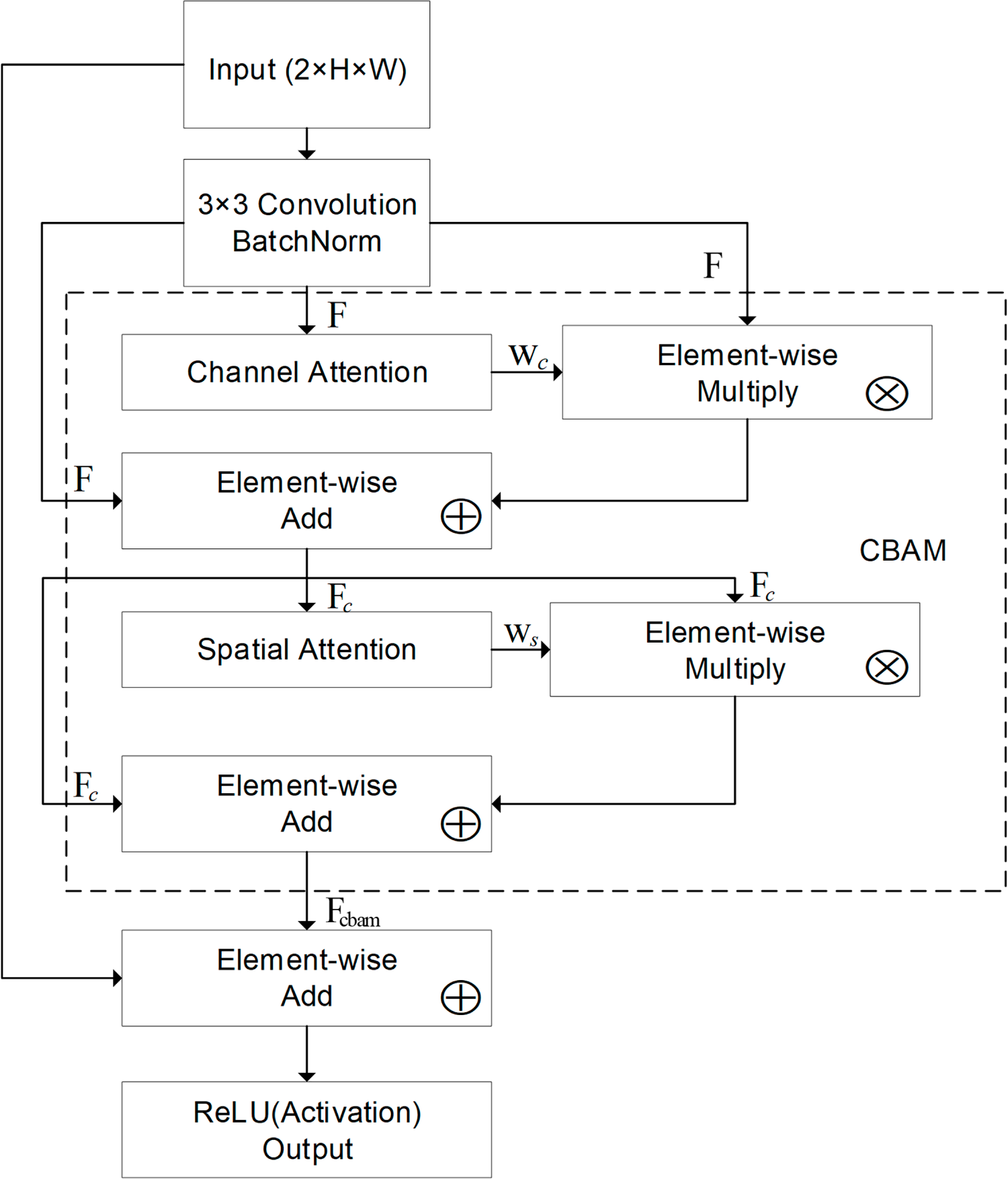
Figure 5: Schematic diagram of Residual Block with CBAM.

Let the block input be X∈RCin×H×W. The main path applies a 3×3 convolution (stride s, padding p=1) followed by batch normalization:

F=BN⁡(Conv3×3,s,p=1⁡(X))∈RCout×H′×W′.(12)

The shortcut is identity when s=1 and Cin=Cout; otherwise, a 1×1 projection with stride s and batch normalization is used to ensure tensor shape compatibility for the residual addition:

S(X)={X,s=1 and Cin=Cout,BN⁡(Conv1×1,s⁡(X)),otherwise.(13)

Next, CBAM is applied to F to produce Fcbam:

•   Channel attention. Global average pooling (GAP) and global max pooling (GMP) over spatial dimensions yield

zavg=GAP⁡(F),zmax=GMP⁡(F)∈RC.(14)

         Both descriptors are passed through shared 1×1 convolutional layers (functionally equivalent to a two-layer multilayer perceptron), and their outputs are summed and squashed by a sigmoid to obtain the channel attention weights:

z^avg=W2ReLU⁡(W1zavg)z^max=W2ReLU⁡(W1zmax),(15)

wc=σ(z^avg+z^max)∈(0,1)C(16)

    where W1 and W2 are shared, learnable 1×1 convolution parameters; ReLU⁡(⋅) denotes the ReLU activation, and σ(⋅) denotes the sigmoid function. Residual-style channel scaling:

Fc=F+F⊙wc(17)

    where ⊙ denotes element-wise multiplication with channel-wise broadcasting.

•   Spatial attention. Channel-wise average and max of Fc are concatenated to form

Q=[Avg⁡(Fc), Max⁡(Fc)]∈R2×H×W,(18)

    which is passed through a 7×7 convolution and a sigmoid:

ws=σ(Conv7×7⁡([Avg⁡(Fc), Max⁡(Fc)]))∈(0,1)1×H×W.(19)

         Residual-style spatial scaling:

Fcbam=Fc+Fc⊙ws.(20)

         Block output. The final output is obtained by residual addition with the shortcut followed by ReLU:

Y=ReLU⁡(Fcbam+S(X)).(21)

3.2.2 SU-Wise Global Pooling and Token Construction

To obtain stable time-frequency features while preserving SU diversity for bidirectional cross-attention, the time-frequency branch applies adaptive Global Average Pooling (GAP) to the third residual block output of each SU and keeps the SU-wise pooled vectors as tokens. Let the output of the third residual block for the m-th SU be

Y3(m)∈RC×H′×W′(m=1,…,M),(22)

and its GAP vector be

gm=GAP⁡(Y3(m))∈RC.(23)

Stacking the SU-wise vectors yields the time-frequency token set

Fcnn=[g1,g2,…,gM]⊤∈RM×C,(24)

which is fed into the BCA module.

3.3 Temporal Branch—Bidirectional GRU

In the presence of GGD noise, the temporal branch aims to enhance noise and signal separability at low SNR. It takes as input the cooperative mean IQ magnitude the complex-domain average across all SUs—to suppress sporadic outliers and to model the temporal evolution of the envelope and phase, thereby providing temporally grounded information of spectrum occupancy under low-SNR conditions.

A gated recurrent unit (GRU) is a recurrent neural architecture that controls information flow via an update gate and a reset gate, enabling selective retention of past context and suppression of spurious fluctuations [36]. For an input xt∈R2 (RMS-normalized magnitude and phase at time t) and hidden state ht−1∈Rh, the single-direction GRU updates are

{zt=σ(Wzxt+Uzht−1+bz),rt=σ(Wrxt+Urht−1+br),h~t=tanh⁡(Whxt+Uh(rt⊙ht−1)+bh),ht=(1−zt)⊙ht−1+zt⊙h~t,(25)

where ht−1,ht∈Rh are the per-direction hidden states; zt,rt∈(0,1)h are the update and reset gates; h~t∈Rh is the candidate state; σ(⋅) and tanh⁡(⋅) denote the sigmoid and hyperbolic tangent functions, respectively; ⊙ denotes element-wise multiplication; and W(⋅)∈Rh×2, U(⋅)∈Rh×h, and b(⋅)∈Rh are learnable parameters. A bidirectional GRU (Bi-GRU) runs two such GRUs in parallel—forward and backward—so that the representation at time t uses both past and future context:

htbi=[h→t; h←t]∈R2h.(26)

In this work, two Bi-GRU layers are stacked (hidden size h=32 per direction), yielding an output tensor:

H=[h0bi,…,hN−1bi]∈RN×2h ⇒ H∈RN×64.(27)

This sequence supplies temporal information to the BCA attention module and, after attention, is mean-pooled over time to form the temporal summary used in the fusion head.

3.4 Bidirectional Cross-Attention (BCA) Module

Under GGD noise and low SNR, a single time-frequency representation can exhibit spurious peaks or textures, while a single temporal representation can suffer short-lived fluctuations. To achieve cross-modal complementarity and suppress noise interference in spectrum sensing, a BCA Attention module is introduced:

•   Path1 (Fcnn as Q, H as K/V). The SU-wise time-frequency tokens Fcnn act as the query (Q) to select informative time steps from the temporal sequence H (keys/values K/V), and aggregate informative temporal evidence to produce an enhanced time-frequency representation F~cnn.

•   Path2 (H as Q, Fcnn as K/V). Each time-step token in H acts as the query (Q) to attend to the SU-wise time-frequency tokens Fcnn (keys/values K/V), thereby injecting global time-frequency evidence into the temporal stream and suppressing GGD-induced short-lived artifacts, yielding an enhanced temporal representation H~.

According to Sections 3.2 to 3.3, the outputs of the time-frequency branch and the temporal branch are denoted by Fcnn∈RM×C and H∈RN×2h, respectively, where M is the number of SUs. Before attention, both streams are mapped into a shared embedding space of dimension D via learned linear projections, as shown in Fig. 6. Here, WQ(1),WK(1),WV(1) are learnable linear projection matrices that map the input tokens to the query, key and value embeddings for Path1, i.e., Q(1),K(1),V(1), respectively. WO(1) is the output projection that maps the attention output back to the feature dimension of the time-frequency stream. Similarly, WQ(2),WK(2),WV(2) and WO(2) are learnable projections for Path2. For Path1, the query, keys, and values are given by

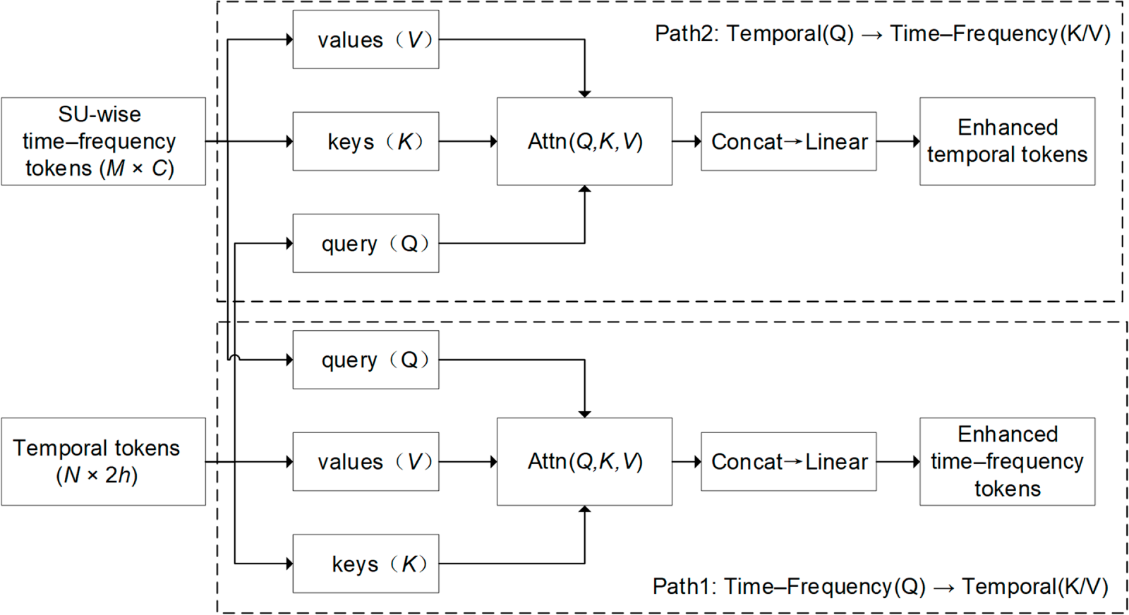
Figure 6: Schematic diagram of BCA module.

{Q(1)=FcnnWQ(1)∈RM×D,K(1)=HWK(1)∈RN×D,V(1)=HWV(1)∈RN×D,(28)

and the enhanced time-frequency tokens are

F~cnn=Attn(Q(1),K(1),V(1))WO(1)∈RM×C.(29)

For Path2, the temporal sequence acts as the query and the time-frequency tokens provide the keys and values:

{Q(2)=HWQ(2)∈RN×D,K(2)=FcnnWK(2)∈RM×D,V(2)=FcnnWV(2)∈RM×D,(30)

leading to an enhanced temporal representation

H~=Attn(Q(2),K(2),V(2))WO(2)∈RN×2h.(31)

In both paths, attention is computed as

Attn⁡(Q,K,V)=softmax(QK⊤d)V,(32)

where d is the per-head dimension and D=Had is the concatenated multi-head embedding dimension with Ha heads. Multi-head attention applies these operations in parallel with different parameter matrices, followed by head concatenation and an output projection.

After multi-head aggregation and output projection, Path1 yields F~cnn∈RM×C and Path2 yields H~∈RN×2h.

To make the bidirectional cross-attention mechanism more intuitive, we visualize the cross-attention weight matrices for the two complementary paths, i.e., Te(Q)→TF(K/V) and TF(Q)→Te(K/V), under both hypotheses H0 and H1 (Figs. 7 and 8). For each hypothesis, the attention maps are averaged over all heads and over up to 200 test samples; the temporal token dimension is mean-pooled into 32 bins, and each row is normalized to sum to one. As shown, the attention allocation exhibits hypothesis-dependent reweighting across SUs and temporal bins, reflecting the mutual calibration behavior enabled by the bidirectional design. Such adaptive reweighting is consistent with the improved robustness observed in our experiments.

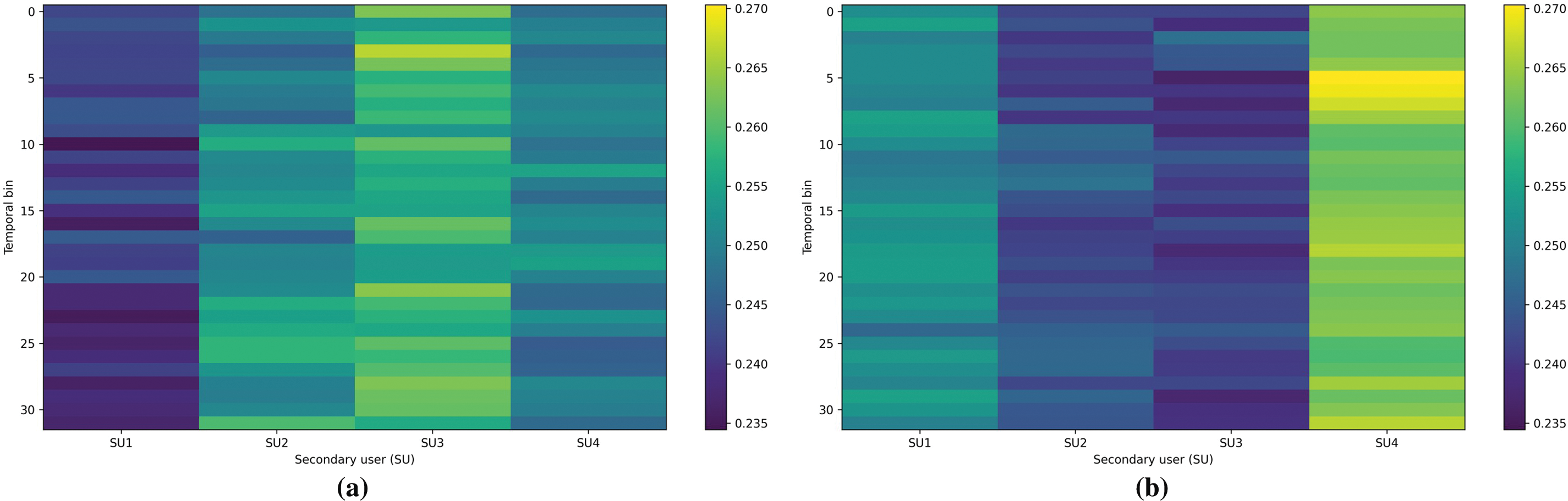
Figure 7: Visualization of the cross-attention weights in the Te(Q)→TF(K/V) path of the proposed BCA module. (a) Te(Q)→TF(K/V) cross-attention under H0 (PU absent); (b) Te(Q)→TF(K/V) cross-attention under H1 (PU present).

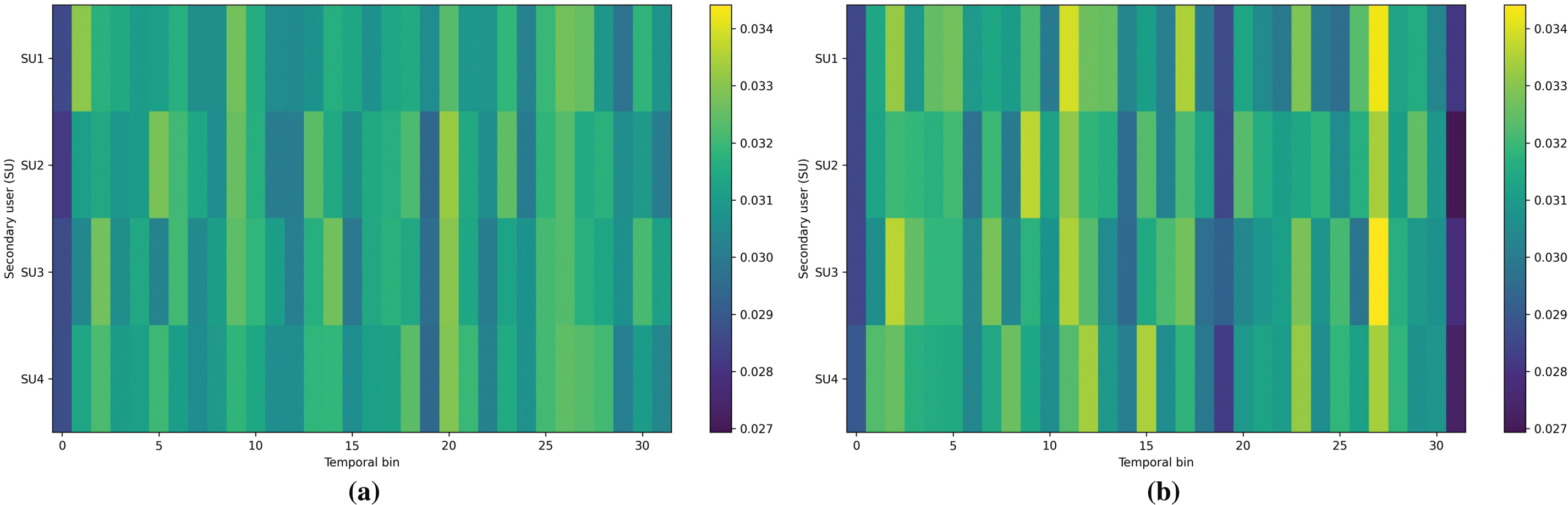
Figure 8: Visualization of the cross-attention weights in the TF(Q)→Te(K/V) path of the proposed BCA module. (a) TF(Q)→Te(K/V) cross-attention under H0 (PU absent); (b) TF(Q)→Te(K/V) cross-attention under H1 (PU present).

3.5 Feature Fusion and Classification

3.5.1 Feature Fusion

The BCA module outputs enhanced time-frequency tokens F~cnn and an enhanced temporal sequence H~={h~t}t=0N−1. For classification, the SU-wise tokens are aggregated by averaging, and the temporal sequence is mean-pooled:

{f¯cnn=1M∑m=1Mf~cnn(m)∈RC,h¯=1N∑t=0N−1h~t∈R2h,(33)

where f~cnn(m) denotes the enhanced token of the m-th SU.

Here, fcnn=1M∑m=1Mgm∈RC denotes the SU-averaged time-frequency descriptor before BCA. The final fusion vector concatenates three complementary components:

z=[fcnn,f¯cnn,h¯].(34)

Thus, z consists of the SU-averaged original time-frequency descriptor fcnn, its BCA-refined counterpart f¯cnn, and the time-frequency guided temporal summary h¯, which together preserve steady global cues, enforce cross-modal consistency, and suppress short-lived artifacts induced by GGD noise.

3.5.2 Normalization and Classifier

Given the fused vector z, the prediction proceeds in three steps:

•   Layer Normalization: feature-wise Layer Normalization (LN) is applied to z to remove modality-dependent scale shifts and stabilize optimization, denoted as LN⁡(z).

•   Two-layer MLP with GELU and Dropout: the normalized vector passes through two linear mappings with a GELU nonlinearity:

v=GELU⁡(W1LN⁡(z)+b1),o=W2v+b2,(35)

    where W1 and b1 are the weight and bias of the first linear projection, and W2 and b2 are those of the second linear layer that produces the two class logits o=[o0,o1]⊤ for (H0,H1). A Dropout layer is inserted between the two linear mappings to mitigate overfitting.

•   Probabilistic output for detection: posterior probabilities are obtained with Softmax:

p^(Hc)=exp⁡(oc)exp⁡(o0)+exp⁡(o1),c∈{0,1}.(36)

3.6 Training and Online Detection

3.6.1 Training

This paper adopts cross-entropy with label smoothing. Let p^(Hc) denote the Softmax posterior and y~ the smoothed target; the loss is

ℒCE=−∑c∈{0,1}y~clog⁡p^(Hc).(37)

Standard optimization and regularization are used to ensure stable convergence.

3.6.2 Threshold Setting and Online Detection

The BCAM-Net output s=p^(H1) is used as the detection statistic. The decision threshold τ∗ is estimated on the training set under H0 so that the empirical false-alarm rate approximately matches the target Pf [37]:

1.    Collect the scores of all training samples labeled H0: SH0={si}i=1n0.

2.    Sort these scores in descending order s(1)≥⋯≥s(n0) and compute k=⌊Pf⋅n0⌋.

3.    Define the threshold as τ∗=s(k).

4.    Using the same τ∗, evaluate the detection probability on the test set as Pd=Pr(s≥τ∗∣H1).

At test time, the fused vector is normalized as LN⁡(z) and passed through the two-layer MLP to obtain the posteriors p^(H0) and p^(H1). Using s=p^(H1) as the detection score, the decision rule is

s={H0,s<τ∗,H1,s≥τ∗.(38)

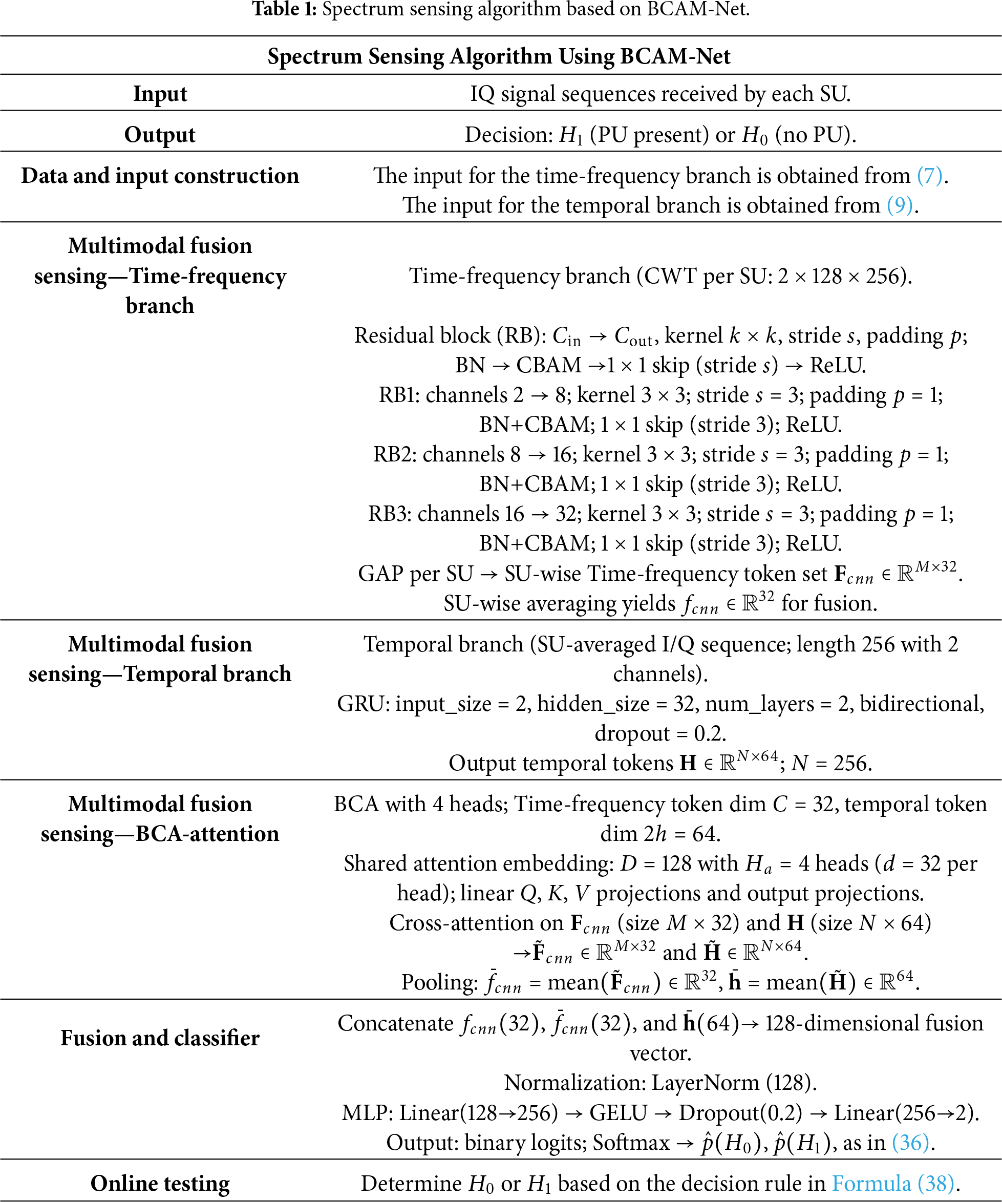
An overview of the complete processing flow is provided in Fig. 9, and the spectrum sensing algorithm based on BCAM-Net is summarized in Table 1. For implementation details, BCAM-Net was trained using AdamW with a learning rate of 0.0008, a batch size of 64, and 40 training epochs.

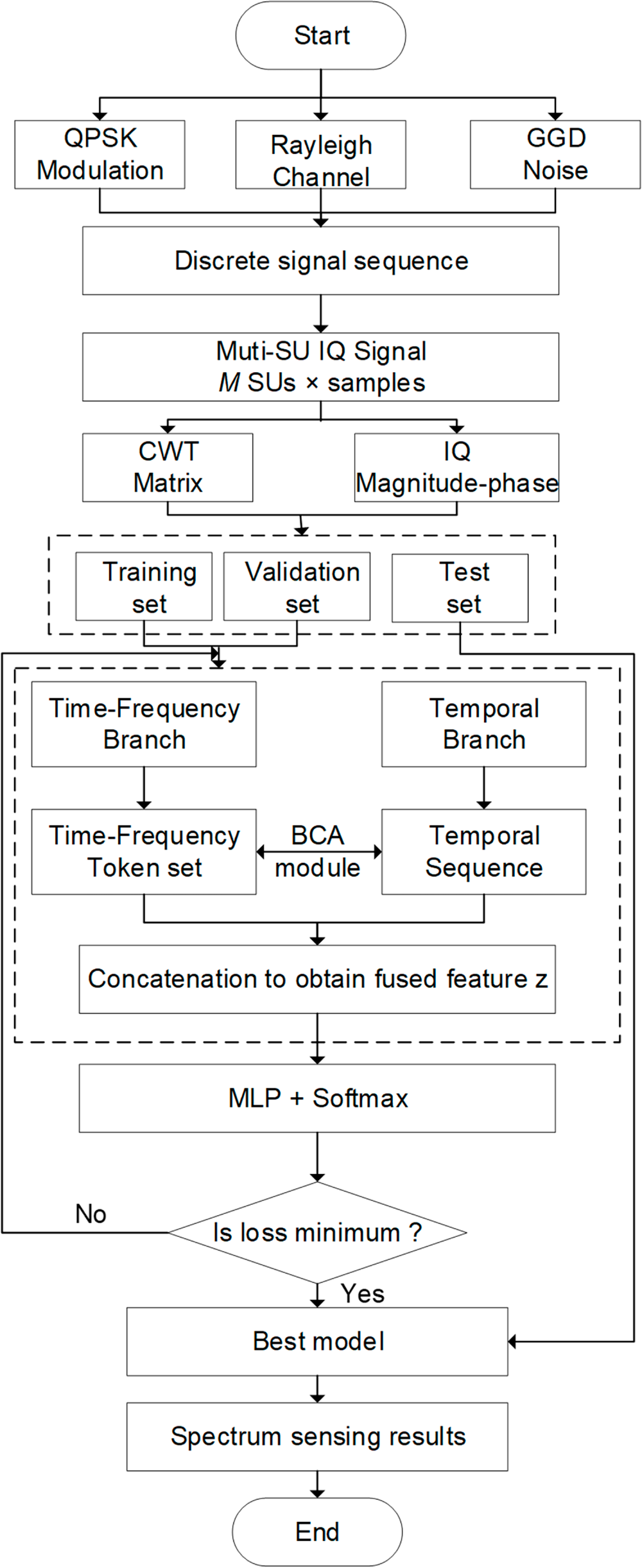
Figure 9: BCAM-Net Algorithm flowchart.

4  Experiments and Performance Evaluation

This section evaluates the proposed spectrum sensing method based on BCAM-Net. The simulation setup and data generation are first described. An ablation study then verifies the contributions of the dual-branch design and BCA attention fusion. Comparisons with representative deep-learning models and classical machine-learning baselines are presented, followed by a robustness study under varying GGD shape parameters. Performance on Real LoRa-Based Spectrum Sensing is then reported. Finally, model complexity is analyzed in terms of parameter count and inference latency.

4.1 Model Simulation Related Parameters

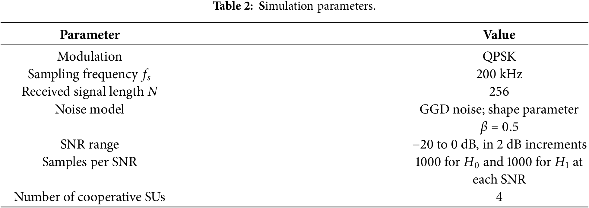
This section evaluates the spectrum sensing approach based on BCAM-Net under GGD noise. The cooperative system comprises one PU and four SUs. The PU employs Quadrature Phase Shift Keying (QPSK) with root-raised-cosine (RRC) pulse shaping, while SU observations are collected over a flat Rayleigh fading channel. Receiver noise in both the null hypothesis H0 (no PU) and the alternative hypothesis H1 (PU present) follows a GGD with shape parameter β=0.5. This value (β=0.5) is adopted as a representative impulsive-noise setting to construct a consistent benchmark for fair baseline comparison and ablation studies. In these experiments, the GGD parameter β is used only to define the noise environment for data generation, and its value is not provided to BCAM-Net or the baseline detectors as an explicit input. The SNR ranges from −20 to 0 dB in 2-dB steps, reflecting the fact that SUs monitor low-power PU uplink signals that suffer severe path loss and fading. At each SNR, each SU acquires 1000 H0 frames (noise only) and 1000 H1 frames (signal plus noise), with 256 complex baseband samples per frame. The resulting dataset is partitioned into training, validation, and test sets with a 7:2:1 split. System parameters are summarized in Table 2.

4.2 Ablation Experiment

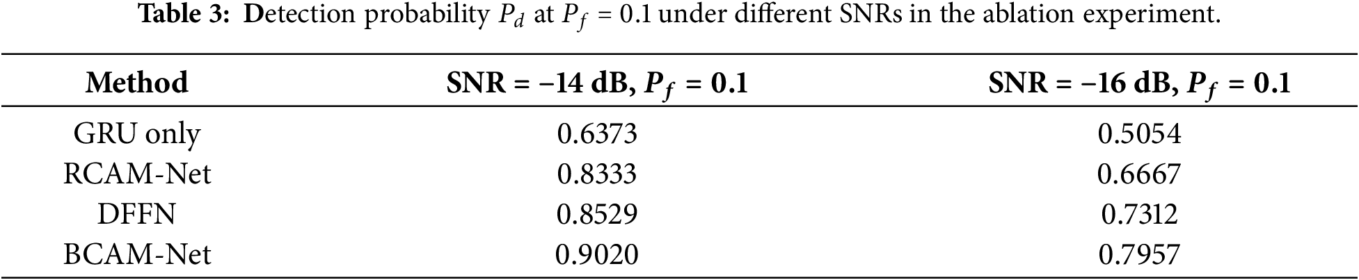
To verify the advantages of BCAM-Net over single-branch models and simple fusion models, ablation experiments were conducted using four comparable configurations: (a) GRU-only (temporal branch only); (b) RCAM-Net (CNN branch only with three residual-CBAM blocks); (c) DFFN (simple concatenation of Dual-branch output); and (d) BCAM-Net. All models are trained and evaluated under identical settings, and the detection probability Pd at a fixed false-alarm rate Pf=0.1 is used as the comparison metric.

Ablation results in Fig. 10 show the detection probability Pd at a fixed false-alarm rate Pf=0.1 across SNRs. All four models exhibit a monotonic increase of Pd with SNR. BCAM-Net achieves the highest Pd in the low-SNR region. Table 3 summarizes representative points at −16 and −14 dB: at Pf=0.1, BCAM-Net reaches Pd=0.7957 at −16 dB, correspondin g to relative improvements of 57.4%, 19.3%, and 8.82% over GRU-only, RCAM-Net, and DFFN, respectively; at −14 dB, BCAM-Net achieves Pd=0.9020, with corresponding improvements of 41.5%, 8.24%, and 5.75%. These results indicate that, compared with single-branch designs and simple concatenation, the dual-branch architecture with BCA attention provides more effective cross-modal integration under GGD (β=0.5) noise and Rayleigh fading.

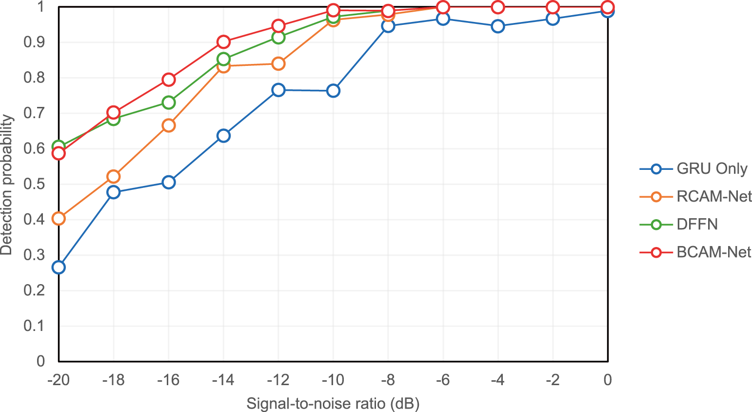
Figure 10: Detection probability under different SNRs in the ablation study at Pf=0.1.

Under the same experimental settings, the contribution of bidirectional interaction in the proposed BCA module is examined via two uni-directional variants, constructed by disabling one cross-attention path while keeping all other components unchanged. Uni-CA (Q = TF, KV = Te) uses the time-frequency tokens Fcnn (output of the time-frequency branch) as queries (Q) and the temporal tokens H (output of the temporal branch) as keys/values (K/V), producing an enhanced time-frequency representation. Conversely, Uni-CA (Q = Te, KV = TF) uses H as queries (Q) and Fcnn as keys/values (K/V), producing an enhanced temporal representation. To further assess the generality of this observation, the same directionality ablation is repeated by replacing the CWT-based input with STFT-based time-frequency features, while keeping all other components and the training protocol unchanged. The results are shown in Fig. 11.

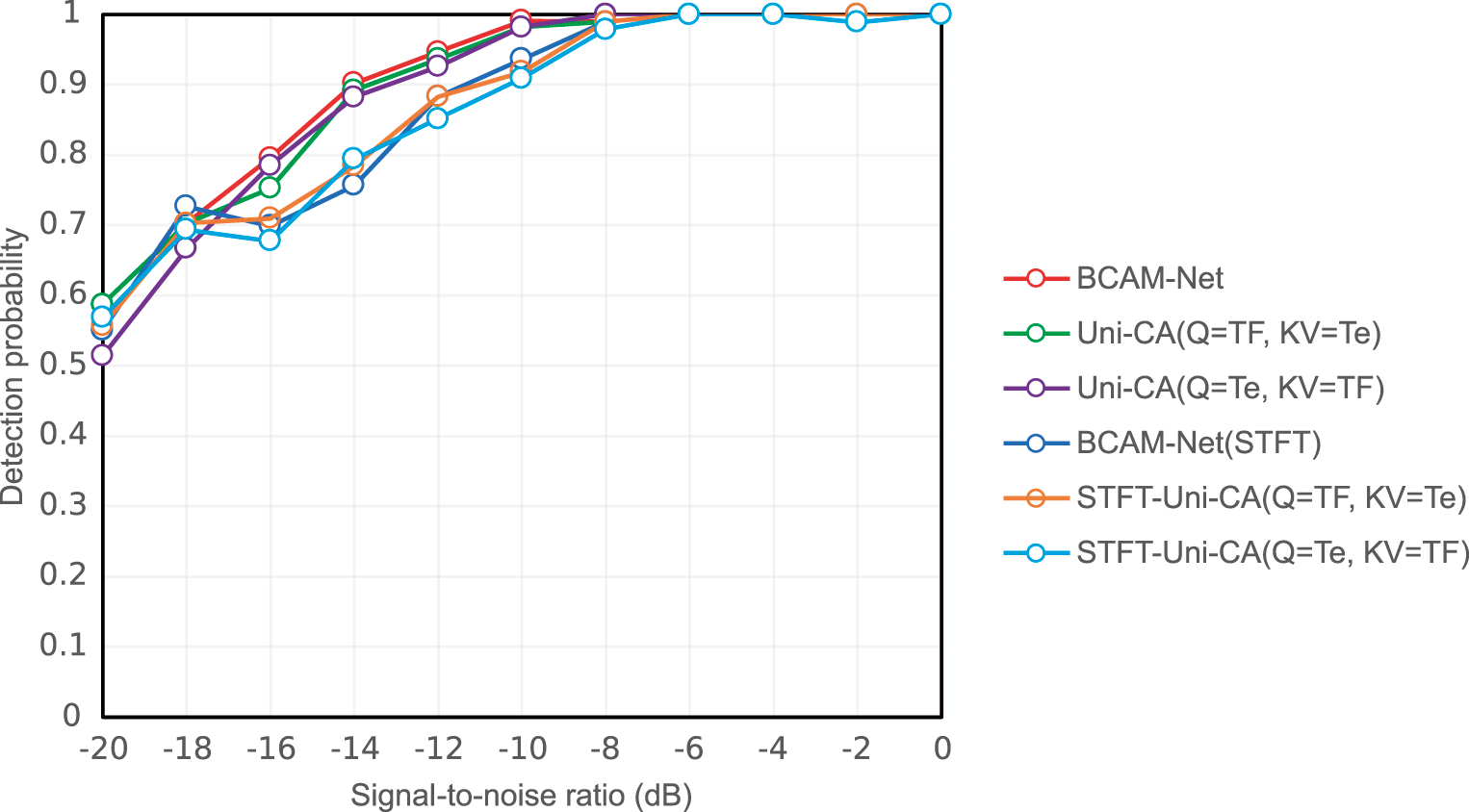
Figure 11: Detection probability under different SNRs for the BCA directionality ablation at Pf=0.1.

As shown in Fig. 11, BCAM-Net generally achieves higher Pd than the two uni-directional variants in the low-SNR regime, whereas the performance gap tends to shrink at higher SNRs where the curves saturate. When replacing CWT with STFT, a similar overall trend is observed, although the curves may intersect at certain SNR points (i.e., the bidirectional model is not strictly dominant at every SNR). These results suggest that the benefit of bidirectional calibration is not tied to a specific time-frequency representation, but is primarily attributed to the cross-modal interaction mechanism.

4.3 Performance Comparison with Other Models

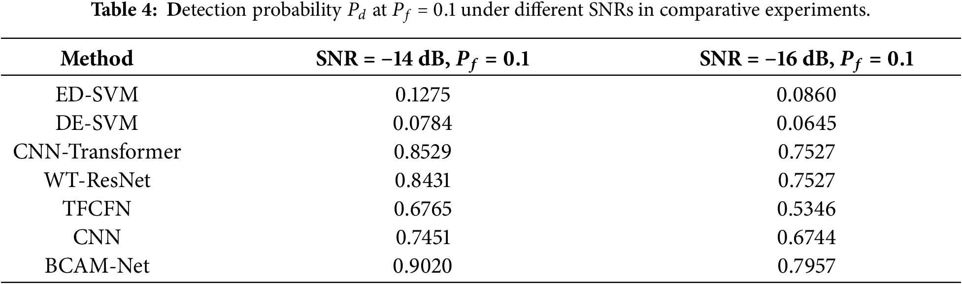
To further evaluate the model performance under identical data and training settings, BCAM-Net was compared with several representative methods. The deep learning models include CNN-Transformer [28], WT-ResNet [25], TFCFN [31], and CNN [24], whose architectural configurations were kept consistent with the original papers. The classical machine learning methods include ED-SVM [19] (an SVM using energy detection features) and DE-SVM [21] (an SVM using GGD differential entropy features).

At a fixed Pf=0.1, the evaluation metric is the detection probability Pd. Fig. 12 shows Pd across SNRs: all methods increase monotonically with SNR, and deep models overall outperform the classical baselines. BCAM-Net and the CNN-Transformer improve earlier in the low-to-mid SNR range (e.g., −16 and −14 dB), WT-ResNet follows, and the CNN is weaker at low SNRs but approaches saturation near −10 dB. Table 4 summarizes the results at −16 and −14 dB; at −14 dB, BCAM-Net exceeds the CNN-Transformer, WT-ResNet,TFCFN, and CNN by 5.75%, 6.98%, 33.3%, and 21.1%, respectively. ED-SVM and DE-SVM lag markedly at low to mid SNRs and show only limited gains at high SNRs. These comparisons indicate that joint cross-modal modeling is more effective than single time-frequency or single temporal features for achieving stable detection under GGD noise (β=0.5) and Rayleigh fading.

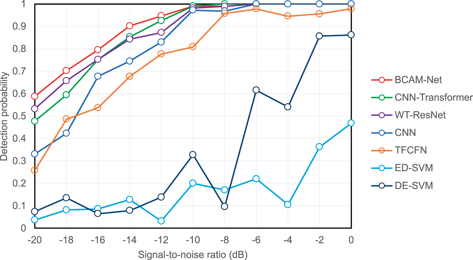
Figure 12: Detection performance comparison of different spectrum sensing models across SNRs at Pf=0.1.

4.4 GGD Noise Shape Parameter Robustness Test

To assess the stability of BCAM-Net under different levels of impulsive noise, for each β∈{0.3,0.6,1.0,1.6,2.0} a separate dataset is generated according to the system and dataset parameters in Table 2. For each fixed β, BCAM-Net is trained, validated, and tested on the corresponding dataset. The evaluation metric is the detection probability Pd at a fixed false-alarm rate Pf=0.1, and the results are shown in Fig. 13.

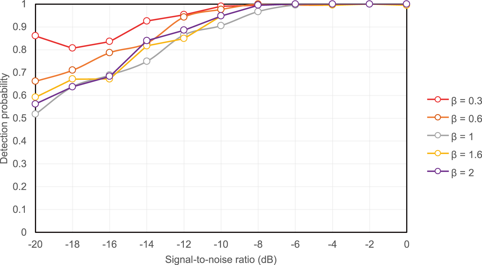
Figure 13: Detection performance of BCAM-Net across SNRs under different β at Pf=0.1.

Across all tested β values, BCAM-Net shows a clear improvement of Pd as SNR increases. The influence of β is most visible in the very low-SNR region (e.g., −20 to −14 dB), where different impulsiveness levels lead to noticeable performance gaps. As SNR increases, the curves progressively converge and enter a high-detection regime: at −10 dB, Pd exceeds 0.90 for all β. Minor local fluctuations may appear under the most impulsive setting (e.g., β=0.3 around −18 to −16 dB), which is expected in heavy-tailed noise where detection is dominated by occasional outliers. Overall, the results indicate that β mainly affects the extreme low-SNR regime, while BCAM-Net remains stable in moderate and high SNR ranges.

Overall, the results indicate that the GGD shape parameter β mainly affects the extreme low-SNR regime, whereas BCAM-Net remains stable in the moderate-to-high SNR range. In particular, for all tested β values, BCAM-Net consistently achieves a high detection probability at −10 dB and above (with Pd>0.9), demonstrating robust and effective spectrum sensing under different noise impulsiveness levels.

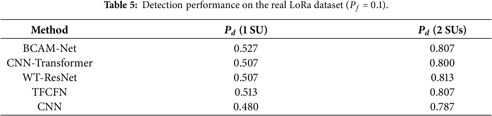
4.5 Performance on Real LoRa-Based Spectrum Sensing

To further verify the practical applicability of the proposed BCAM-Net, additional experiments were conducted on a publicly available real SDR dataset reported in [38], which contains over-the-air IQ recordings of uplink LoRa transmissions and background noise captured using an RTL-SDR. In this dataset, the LoRa signals are centered at 868.1 MHz with a 125 kHz bandwidth (SF7 and SF12, i.e., spreading factor 7 and 12) [38]. Since the dataset provides recordings collected under different receive-attenuation settings, two recordings with different attenuation levels were selected and treated as two SU observations to construct an approximate 2-SU cooperative sensing scenario. Note that this setting approximates heterogeneous SU sensing qualities using different attenuation levels rather than two synchronized receivers.

For each SU and each hypothesis, the baseband IQ samples were segmented into frames of 256 samples to form a binary detection dataset (hypothesis H0: noise only; hypothesis H1: LoRa plus noise). A total of 1500 frames per hypothesis were extracted for each SU, and the resulting dataset was split into training, validation and test subsets with a ratio of 7:2:1.

Table 5 summarizes the detection performance on the real LoRa dataset at Pf=0.1 under single-SU and 2-SU settings. As shown in Table 5, all methods benefit from cooperation: Pd increases markedly when the number of SUs grows from 1 to 2, which is consistent with the expected cooperative gain obtained by aggregating multiple observations in practical sensing scenarios. BCAM-Net achieves competitive detection performance, with Pd improving from 0.527 (1 SU) to 0.807 (2 SUs) at Pf=0.1. These real-data results support the practical feasibility of the proposed IoT-oriented spectrum sensing framework. This experiment mainly serves as a feasibility validation on real SDR measurements; extending the evaluation to larger-scale real deployments remains an important direction for future work.

4.6 Complexity Analysis

This section analyzes model complexity in terms of parameter count (Params, in millions) and per-frame inference latency (ms/frame). All results were obtained under identical hardware and settings on an NVIDIA RTX 4090D (24 GB) GPU with an AMD EPYC 9754 host. As shown in Fig. 14, BCAM-Net has 0.12M parameters and 0.0313 ms/frame latency, offering low inference cost while remaining lightweight. CNN-Transformer [28] requires 0.92M parameters with 0.7601 ms/frame latency, both substantially higher than BCAM-Net. WT-ResNet [25] uses 0.14M parameters and attains the lowest latency (0.0115 ms/frame), whereas the two-layer CNN [24] has 0.11M parameters but a relatively high latency of 0.4412 ms/frame.

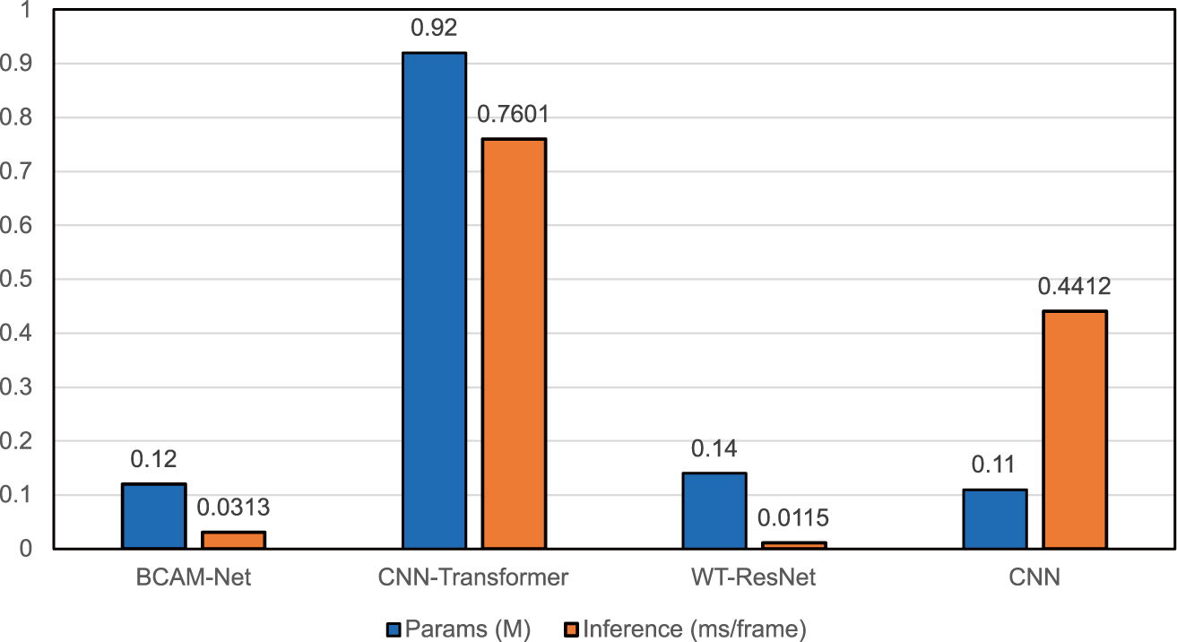
Figure 14: BCAM-Net complexity analysis comparison.

Based on the detection performance analysis above, BCAM-Net achieves a favorable balance between performance and efficiency under our unified GPU setting. Moreover, with 0.12M parameters, the model-weight storage is approximately 0.48 MB in FP32 (0.24 MB in FP16), which suggests potential suitability for memory-constrained edge deployment. Detailed on-device benchmarking of latency, energy consumption, and memory usage on representative edge platforms will be investigated in future work.

Nevertheless, practical deployments may involve additional challenges. In practical deployments, SUs may experience heterogeneous received SNRs, which can make cooperative fusion sensitive to unreliable observations. For controlled comparison, the current experiments assume identical SNR across SUs. Extending BCAM-Net to explicitly handle heterogeneous-SNR scenarios remains an important direction for future work.

5  Conclusion

This paper investigates spectrum sensing for IoT-oriented networks under GGD noise, where heavy-tailed disturbances can significantly degrade the reliability of conventional sensing pipelines. To address this challenge, BCAM-Net is proposed as a multimodal framework that jointly exploits time-frequency and temporal information. Specifically, BCAM-Net learns CWT-based time-frequency features through a time-frequency branch and learns magnitude-phase sequence features through a temporal branch; meanwhile, a BCA module is introduced to achieve explicit mutual calibration between the two modalities, thereby enhancing cross-modal feature fusion. In addition, BCAM-Net adopts a lightweight design, maintaining a low parameter count and low inference latency to improve practicality for real-world deployment scenarios.

Extensive experiments demonstrate that, at a fixed false-alarm probability Pf, BCAM-Net consistently improves detection performance compared with single-branch baselines, simple concatenation-based fusion, and uni-directional cross-attention variants. Moreover, BCAM-Net shows stable behavior across different GGD shape parameters, indicating enhanced robustness to variations in noise impulsiveness. The complexity analysis further confirms a favorable accuracy-efficiency trade-off, suggesting that BCAM-Net is promising for resource-constrained IoT devices.

However, some limitations still exist. First, the performance still degrades in extremely low-SNR regimes, where both temporal and time-frequency cues become weak and attention reweighting may be less discriminative. Second, the evaluation assumes the same received SNR for all SUs, which may differ from practical networks where per-SU SNRs vary due to shadowing, fading, and hardware diversity. Third, the generalization capability to a broader range of modulation types and more complex signal environments has not been fully validated.

Future work will focus on improving detection performance in extremely low-SNR conditions, extending the evaluation to more realistic scenarios with heterogeneous SU sensing qualities, further validating the proposed method under broader signal settings and real-world SDR measurements, and benchmarking latency, energy consumption, and memory usage on representative edge platforms.

Acknowledgement: Not applicable.

Funding Statement: This research was supported in part by JSPS Grants-in-Aid for Scientific Research 25K07742 and 25K23457.

Author Contributions: The authors confirm contribution to the paper as follows: study conception and design: Yuzhou Han; data collection and dataset preparation: Yuzhou Han; analysis and interpretation of results: Yuzhou Han; draft manuscript preparation: Yuzhou Han. Osamu Muta, Ahmad Gendia, Zhuoran Li and Teruji Ide contributed through technical discussions and provided critical revisions and key suggestions on the initial draft that improved the manuscript. Ahmad Gendia also provided guidance on the experimental design and assisted with English grammar polishing. All authors reviewed and approved the final version of the manuscript.

Availability of Data and Materials: The data supporting the findings of this study are available from the corresponding author, Yuzhou Han, upon reasonable request.

Ethics Approval: Not applicable.

Conflicts of Interest: The authors declare no conflicts of interest.

References

1. Nguyen DC, Ding M, Pathirana PN, Seneviratne A, Li J, Niyato D, et al. 6G Internet of Things: a comprehensive survey. IEEE Internet Things J. 2022;9(1):359–83. doi:10.1109/JIOT.2021.3103320. [Google Scholar] [CrossRef]

2. Liu X, Jia M, Zhou M, Wang B, Durrani TS. Integrated cooperative spectrum sensing and access control for cognitive industrial Internet of Things. IEEE Internet Things J. 2023;10(3):1887–96. doi:10.1109/JIOT.2021.3137408. [Google Scholar] [CrossRef]

3. Wang J, Jiang W, Wang H, Huang Y, Chen R, Lin R. Multiband spectrum sensing and power allocation for a cognitive radio-enabled smart grid. Sensors. 2021;21(24):8384. doi:10.3390/s21248384. [Google Scholar] [PubMed] [CrossRef]

4. Rodríguez-Piñeiro J, Wei Z, Wang J, Gutiérrez CA, Correia LM. 6G-enabled vehicle-to-everything communications: current research trends and open challenges. IEEE Open J Veh Technol. 2025;6:2358–91. doi:10.1109/OJVT.2025.3599570. [Google Scholar] [CrossRef]

5. Parvini M, Zarif AH, Nouruzi A, Mokari N, Javan MR, Abbasi B, et al. Spectrum sharing schemes from 4G to 5G and beyond: protocol flow, regulation, ecosystem, and economics. IEEE Open J Commun Soc. 2023;4:464–517. doi:10.1109/OJCOMS.2023.3238569. [Google Scholar] [CrossRef]

6. Nasser A, Al Haj Hassan H, Abou Chaaya J, Mansour A, Yao K-C. Spectrum sensing for cognitive radio: recent advances and future challenge. Sensors. 2021;21(7):2408. doi:10.3390/s21072408. [Google Scholar] [PubMed] [CrossRef]

7. Liu X, Jia M. Intelligent spectrum resource allocation based on joint optimization in heterogeneous cognitive radio. IEEE Trans Emerg Top Comput Intell. 2020;4(1):5–12. doi:10.1109/TETCI.2018.2865630. [Google Scholar] [CrossRef]

8. Wasilewska M, Bogucka H, Poor HV. Secure federated learning for cognitive radio sensing. IEEE Commun Mag. 2023;61(3):68–73. doi:10.1109/MCOM.001.2200465. [Google Scholar] [CrossRef]

9. Ali A, Hamouda W. Advances on spectrum sensing for cognitive radio networks: theory and applications. IEEE Commun Surv Tutor. 2017;19(2):1277–304. doi:10.1109/COMST.2016.2631080. [Google Scholar] [CrossRef]

10. Gaiera B, Patel DK, Soni B, López-Benítez M. Performance evaluation of improved energy detection under signal and noise uncertainties in cognitive radio networks. In: 2019 IEEE International Conference on Signals and Systems (ICSigSys). Piscataway, NJ, USA: IEEE; 2019. p. 131–7. doi:10.1109/ICSIGSYS.2019.8811079. [Google Scholar] [CrossRef]

11. Arjoune Y, Kaabouch N. A comprehensive survey on spectrum sensing in cognitive radio networks: recent advances, new challenges, and future research directions. Sensors. 2019;19(1):126. doi:10.3390/s19010126. [Google Scholar] [PubMed] [CrossRef]

12. Yan X, Liu G, Wu H-C, Zhang G, Wang Q, Wu Y. Robust modulation classification over α-stable noise using graph-based fractional lower-order cyclic spectrum analysis. IEEE Trans Veh Technol. 2020;69(3):2836–49. doi:10.1109/TVT.2020.2965137. [Google Scholar] [CrossRef]

13. Mehrabian A, Sabbaghian M, Yanikomeroglu H. Spectrum sensing for symmetric α-stable noise model with convolutional neural networks. IEEE Trans Commun. 2021;69(8):5121–35. doi:10.1109/TCOMM.2021.3070892. [Google Scholar] [CrossRef]

14. Agrawal SK, Samant A, Yadav SK. Spectrum sensing in cognitive radio networks and metacognition for dynamic spectrum sharing between radar and communication system: a review. Phys Commun. 2022;52:101673. doi:10.1016/j.phycom.2022.101673. [Google Scholar] [CrossRef]

15. Salameh HB, Hussienat A. ML-driven feature-based spectrum sensing for NOMA signal detection in spectrum-agile IoT networks under fading channels. IEEE Sens J. 2025;25(13):25963–71. doi:10.1109/JSEN.2025.3569620. [Google Scholar] [CrossRef]

16. Zhang Y, Luo Z. A deep-learning-based method for spectrum sensing with multiple feature combination. Electronics. 2024;13(14):2705. doi:10.3390/electronics13142705. [Google Scholar] [CrossRef]

17. Janu D, Singh K, Kumar S. Machine learning for cooperative spectrum sensing and sharing: a survey. Trans Emerg Telecommun Technol. 2022;33(1):e4352. doi:10.1002/ett.4352. [Google Scholar] [CrossRef]

18. Wu Q, Ng BK, Lam C-T. Energy-efficient cooperative spectrum sensing using machine learning algorithm. Sensors. 2022;22(21):8230. doi:10.3390/s22218230. [Google Scholar] [PubMed] [CrossRef]

19. Saber M, El Rharras A, Saadane R, Aroussi HK, Wahbi M. Artificial neural networks, support vector machine and energy detection for spectrum sensing based on real signals. Int J Commun Netw Inf Secur. 2019;11(1):52–60. doi:10.17762/ijcnis.v11i1.3718. [Google Scholar] [CrossRef]

20. Varma AK, Mitra D. Statistical feature-based SVM wideband sensing. IEEE Commun Lett. 2020;24(3):581–4. doi:10.1109/LCOMM.2019.2959355. [Google Scholar] [CrossRef]

21. Saravanan P, Chandra SS, Upadhye A, Gurugopinath S. A supervised learning approach for differential entropy feature-based spectrum sensing. In: 2021 Sixth International Conference on Wireless Communications, Signal Processing and Networking (WiSPNET). Piscataway, NJ, USA: IEEE; 2021. p. 395–9. doi:10.1109/WiSPNET51692.2021.9419447. [Google Scholar] [CrossRef]

22. Kumar A, Gaur N, Chakravarty S, Alsharif MH, Uthansakul P, Uthansakul M. Analysis of spectrum sensing using deep learning algorithms: CNNs and RNNs. Ain Shams Eng J. 2024;15(3):102505. doi:10.1016/j.asej.2023.102505. [Google Scholar] [CrossRef]

23. Wang L, Hu J, Zhang C, Jiang R, Chen Z. Deep learning models for spectrum prediction: a review. IEEE Sens J. 2024;24(18):28553–75. doi:10.1109/JSEN.2024.3416738. [Google Scholar] [CrossRef]

24. Chen Z, Xu Y-Q, Wang H, Guo D. Deep STFT-CNN for spectrum sensing in cognitive radio. IEEE Commun Lett. 2021;25(3):864–8. doi:10.1109/LCOMM.2020.3037273. [Google Scholar] [CrossRef]

25. Zhen P, Zhang B, Chen Z, Guo D, Ma W. Spectrum sensing method based on wavelet transform and residual network. IEEE Wirel Commun Lett. 2022;11(12):2517–21. doi:10.1109/LWC.2022.3207296. [Google Scholar] [CrossRef]

26. Xu L, Gao Z, Li Y, Gulliver TA. Cross-domain intelligent cooperative spectrum sensing algorithm based on Federated Learning and Swin-Transformer neural network. Eng Appl Artif Intell. 2025;157:111370. doi:10.1016/j.engappai.2025.111370. [Google Scholar] [CrossRef]

27. Varma DP, Yeduri SR, Yakkati RR, Boddu AB, Cenkeramaddi LR. Wireless technology identification using continuous wavelet transform and deep learning. IEEE Sens J. 2025;25(13):23284–91. doi:10.1109/JSEN.2024.3467681. [Google Scholar] [CrossRef]

28. Fang X, Jin M, Guo Q, Jiang T. CNN-transformer-based cooperative spectrum sensing in cognitive radio networks. IEEE Wirel Commun Lett. 2025;14(5):1576–80. doi:10.1109/LWC.2025.3550536. [Google Scholar] [CrossRef]

29. Gao Z, Li Y, Chen Z, Asif M, Xu L, Li X, et al. Intelligent spectrum sensing of consumer IoT based on GAN-GRU-YOLO. IEEE Trans Consum Electron. 2024;70(3):6140–8. doi:10.1109/TCE.2024.3418103. [Google Scholar] [CrossRef]

30. Zhang W, Wang Y, Chen X, Cai Z, Tian Z. Spectrum transformer: an attention-based wideband spectrum detector. IEEE Trans Wirel Commun. 2024;23(9):12343–53. doi:10.1109/TWC.2024.3391515. [Google Scholar] [CrossRef]

31. Xi H, Guo W, Yang Y, Yuan R, Ma H. Cross-attention mechanism-based spectrum sensing in generalized Gaussian noise. Sci Rep. 2024;14(1):23261. doi:10.1038/s41598-024-74341-4. [Google Scholar] [PubMed] [CrossRef]

32. Dao Y, Liang B, Hao L, Feng S, Wei S, Dai W, et al. Radio frequency interference identification using dual cross-attention and multi-scale feature fusing. Astron Comput. 2024;49:100881. doi:10.1016/j.ascom.2024.100881. [Google Scholar] [CrossRef]

33. Xing S, Wang Z, Zhao R, Guo X, Liu A, Liang W. Time-frequency-domain fusion cross-attention fault diagnosis method based on dynamic modeling of bearing rotor system. Appl Sci. 2025;15(14):7908. doi:10.3390/app15147908. [Google Scholar] [CrossRef]

34. Kockaya K, Develi I. Spectrum sensing in cognitive radio networks: threshold optimization and analysis. J Wirel Commun Netw. 2020;2020:255. doi:10.1186/s13638-020-01870-7. [Google Scholar] [CrossRef]

35. Gurugopinath S, Muralishankar R, Shankar HN. Differential entropy-driven spectrum sensing under generalized Gaussian noise. IEEE Commun Lett. 2016;20(7):1321–4. doi:10.1109/LCOMM.2016.2564968. [Google Scholar] [CrossRef]

36. Bai X, Xu J, Fang F, Wang X, Wang S. A multi-feature spectrum sensing algorithm based on GRU-AM. IEEE Wirel Commun Lett. 2025;14(7):2129–33. doi:10.1109/LWC.2025.3564053. [Google Scholar] [CrossRef]

37. Cai L, Cao K, Wu Y, Zhou Y. Spectrum sensing based on spectrogram-aware CNN for cognitive radio network. IEEE Wirel Commun Lett. 2022;11(10):2135–9. doi:10.1109/LWC.2022.3194735. [Google Scholar] [CrossRef]

38. Fontaine J, Shahid A, Elsas R, Seferagic A, Moerman I, de Poorter E. Multi-band sub-GHz technology recognition on NVIDIA’s Jetson Nano. In: 2020 IEEE 92nd Vehicular Technology Conference (VTC2020-Fall). Piscataway, NJ, USA: IEEE; 2020. p. 1–7. doi:10.1109/VTC2020-Fall49728.2020.9348566. [Google Scholar] [CrossRef]