Acoustic-Emission–Driven Pipeline Leak Detection Using Wavelet Time–Frequency Maps and Inception-V3 Deep Network

1  Introduction

Pipelines often operate under high-pressure or long-distance conditions for extended periods, making them susceptible to corrosion, aging, mechanical damage, and installation defects, which may result in leakage [1]. In the petroleum and natural gas industries, leakage not only leads to resource waste but may also cause environmental pollution, fires, or even explosions, posing serious threats to human safety. Therefore, implementing efficient and reliable methods for pipeline leakage monitoring and identification is a crucial measure to ensure industrial operational safety [2]. Currently, commonly used leakage detection techniques include manual inspection, olfactory sensors, infrared thermography, negative pressure wave analysis, and AE detection. Among these methods, the AE technique has become an efficient and cost-effective solution due to its real-time capability, high sensitivity, non-invasiveness, and ability to detect multiple types of defects [3].

In recent years, deep learning, as an important branch of artificial intelligence, has demonstrated remarkable advantages in fault diagnosis and pattern recognition [4,5]. Convolutional neural networks (CNNs), with their strong capabilities for automatic feature extraction and nonlinear representation, can effectively identify complex signal characteristics and improve diagnostic accuracy [6]. For instance, Huang et al. [7] developed a temporal convolutional network (TCN)–based model for weld crack recognition and leakage rate prediction, achieving accurate estimation of leakage rates from AE signals. Zhang et al. [8] proposed a contactless pipeline leakage detection system based on a novel semantic segmentation network, WDA-Net, which adopts a CNN–Transformer hybrid encoder and an efficient feature-fusion decoder to robustly segment weak pipeline leakage defects under complex illumination conditions. However, for AE signals, traditional feature extraction methods—such as mean, standard deviation, peak value, and frequency band energy—are often sensitive to noise and reliant on manual feature design, making it difficult to adequately characterize their non-stationary properties and local variations [9,10]. To address this issue, time–frequency analysis methods have been introduced for leakage signal feature extraction to reveal the temporal evolution of frequency components. Among them, the wavelet transform is a typical time–frequency analysis tool with excellent time–frequency localization capability, providing high time resolution in high-frequency regions and high frequency resolution in low-frequency regions, thereby enabling accurate capture of transient changes and local details [11]. Saleem et al. [12] employed CWT to process AE signals and constructed a detection model by integrating a CNN-LSTM network with a genetic algorithm. Validation on real-world datasets demonstrated an accuracy of 99.69% in the binary classification task.

Based on the above studies, this paper focuses on pipeline leakage detection by employing the CWT to process the non-stationary characteristics of AE signals and combining it with the automatic feature extraction capability of deep learning. A pipeline leakage state recognition method based on wavelet time–frequency maps and the Inception-V3 network is proposed, achieving high accuracy and strong robustness in leakage detection under various operating conditions. The proposed method provides an efficient and reliable solution for pipeline leakage monitoring under complex industrial environments.

2  Fundamental Principle Analysis

2.1 Continuous Wavelet Transform

The time-frequency analysis method can effectively reveal the variation of signal frequency over time. The time-frequency maps generated by the CWT simultaneously display the signal’s time, frequency, and energy distribution information. With its multi-resolution analysis capability, CWT can adaptively characterize the local features of a signal at different scales—providing higher time resolution in high-frequency regions and higher frequency resolution in low-frequency regions. This allows for more accurate capture of instantaneous variations and fine details of non-stationary signals [13].

Therefore, CWT has been widely applied to time-frequency feature extraction and pattern recognition of non-stationary signals. For example, Song et al. [14] proposed a CWT–CNN-based method for leak size identification in non-metallic pipelines. In their approach, AE signals are first denoised and then converted into CWT time-frequency maps, which are used as inputs to a CNN. The proposed method achieved excellent performance, with a maximum identification accuracy of 95%. Siddique et al. [15] transformed AE signals into enhanced leakage-induced scalograms (ELIS), which preserve both time- and frequency-domain information and effectively improve identification accuracy in pipeline monitoring.

For any integrable function f(t)∈L2(R), the CWT is defined as:

Wf(a,b)=⟨f,ψa,b⟩=|a|−12∫Rf(t)ψ∗(t−ba)dt(1)

where ψ is the mother wavelet function; a is the scale factor, which adjusts the frequency of the wavelet; b is the translation factor, which controls the time-domain position of the wavelet; and ψ∗ denotes the complex conjugate of the mother wavelet.

2.2 Inception-V3

There are many architectures based on CNN for image classification, such as AlexNet, VGGNet, and GoogLeNet. Compared with AlexNet and VGGNet, GoogLeNet (which adopts the Inception architecture) achieves a lower error rate and a much deeper network while using only about 5 million parameters—approximately 12 times fewer than AlexNet and nearly 30 times fewer than VGGNet. This relatively small number of parameters allows the network to be efficiently trained on various datasets while maintaining high performance.

The main characteristics of the GoogLeNet architecture are as follows:

•   The introduction of the Inception module enables the fusion of multiscale feature information.

•   1 × 1 convolution kernels are employed for dimensionality reduction and feature mapping.

•   Two auxiliary classifiers are added to assist the training process.

•   An average pooling layer is used to reduce the total number of model parameters.

The Inception-V3 model is one of the most commonly used deep CNN architectures for image classification. It incorporates a specific type of Inception module, which can be regarded as a smaller convolutional sub-network within the main network. Compared with traditional convolutional layers, this structure exhibits better learning capability and effectively addresses several limitations of conventional networks, such as excessive parameters, overfitting, gradient vanishing, and computational inefficiency.

The most significant improvement in the Inception-V3 model is the factorization strategy, as illustrated in Fig. 1. In this architecture, a 3 × 3 convolution kernel is decomposed into two 3 × 1 and 1 × 3 convolution kernels, which not only accelerate computation but also increase network depth and nonlinearity, thereby enhancing the model’s generalization ability. Compared with other large-scale convolutional networks, the Inception-V3 model demonstrates stronger feature extraction capability, faster training speed, and higher classification accuracy. It has achieved excellent performance in various applications, including cervical cancer cell recognition, traffic sign classification, and waste sorting.

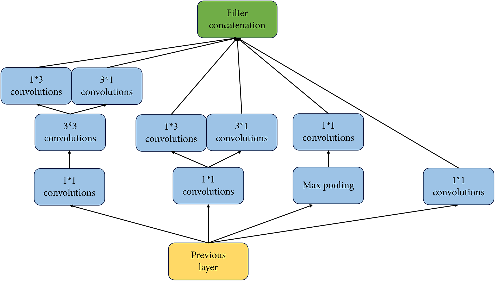
Figure 1: Inception v3 model.

3  Pipeline Acoustic Emission Signal Characteristics

3.1 Experimental Setup

To simulate different leakage conditions in pipelines, an experimental platform was constructed in the laboratory. The experimental setup for pipeline leakage detection is shown in Figs. 2 and 3. The main equipment includes an AE detector, sensors, a computer, an air compressor, and a test pipeline. The total length of the pipeline is 5 m, consisting of a 200 mm–diameter steel straight pipe and a curved pipe section. The pipeline is equipped with weld joints and valves of various types, allowing the simulation of multiple operating conditions.

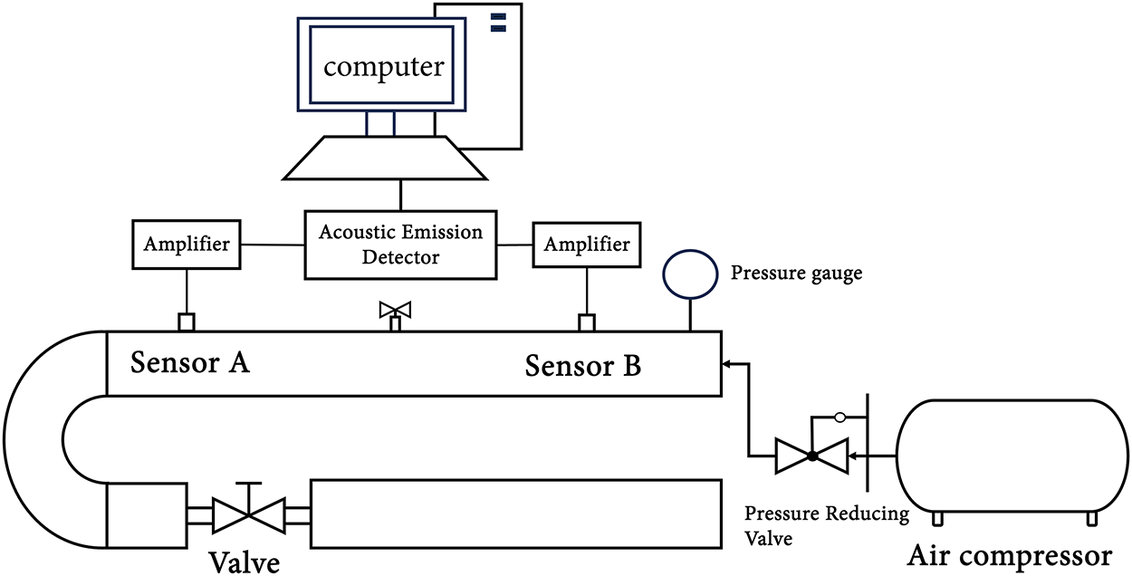
Figure 2: Schematic diagram of the experimental platform.

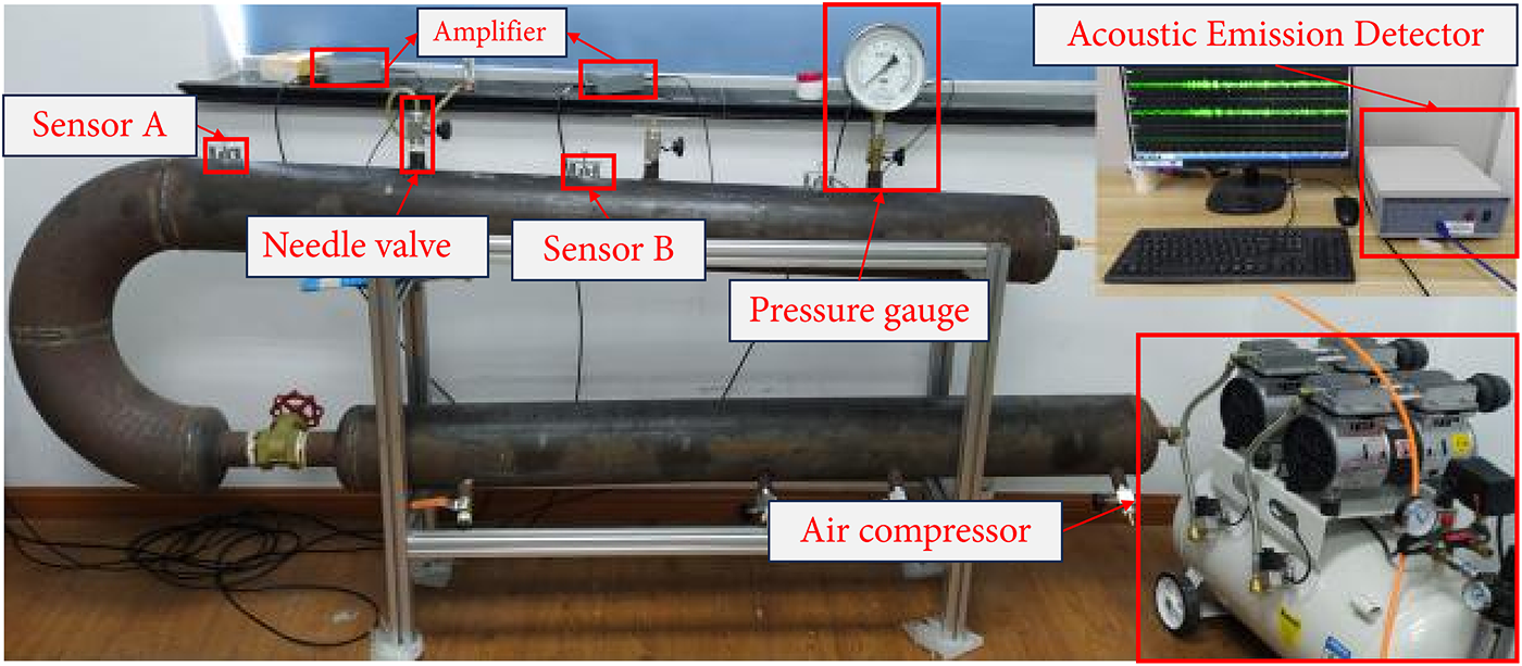
Figure 3: Physical diagram of the experimental platform.

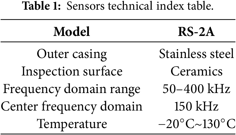
On the far right of the setup, an air compressor provides the air source for the pipeline. A pressure-reducing valve is installed between the compressor and the pipeline to regulate the inlet pressure of the gas. A pressure gauge is mounted at the upper right of the apparatus to monitor the internal pressure of the pipeline and prevent accidents. Leakage points are designed on the pipe wall, and by adjusting the needle valve opening, different leakage states can be effectively simulated. The selected sensor is a wideband RS-2A resonant-type AE sensor, its technical specifications are listed in Table 1.

The data acquisition device used in this study is a DS5 AE acquisition system, which features long-term signal recording and storage capabilities, as well as a step-by-step playback function that facilitates waveform and frequency analysis.

During the data acquisition process, the internal gas pressure of the pipeline was strictly stabilized at 0.5 MPa via the pressure-reducing valve. Sensors A and B were mounted on the pipeline surface using magnetic hold-downs, located 0.25 m upstream and 0.25 m downstream from the leakage point, respectively. The experiment was conducted in a laboratory environment with an average background noise level of approximately 35 dB, which includes noise from the air compressor and ambient environment.

3.2 Frequency Domain Characteristics of Acoustic Emission Signals from Pipeline Leakage

Based on the leakage point shown in Fig. 3, three leakage conditions were simulated with leakage rates of 0, 500, and 1000 mL/min, respectively. The corresponding AE signals were collected at a sampling frequency of 2.5 MHz and a recording duration of 1000 ms. The acquired signals were then processed using the Fast Fourier Transform (FFT) to obtain their frequency spectra.

To more precisely identify the characteristic leakage frequency band, the frequency spectra corresponding to the three leakage states were magnified within the 0–400 kHz range for detailed examination. The frequency-domain plots generated using MATLAB are shown in Fig. 4.

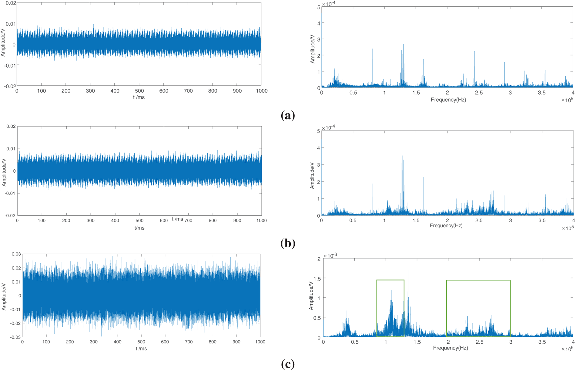
Figure 4: Time-domain and frequency-domain diagrams for three leakage conditions. (a) 0 mL/min; (b) 500 mL/min; (c) 1000 mL/min.

As observed from the time-domain waveforms in Fig. 4, even in the absence of leakage, the AE system captured significant ambient noise. A comparison between the non-leakage and 500 mL/min leakage conditions reveals that the two waveforms exhibit minimal visible differences, indicating that the leakage signal is masked by background noise. However, when the leakage rate increases to 1000 mL/min, the amplitude of the waveform becomes significantly higher than that observed under the other two conditions.

In the frequency domain, several sharp spectral peaks are present under the non-leakage condition. These are attributed to external disturbances such as roadwork, vehicle movement, and fountain noise, all contributing to non-stationary background interference. By comparing the frequency domain plots of 0 mL/min leakage and 500 mL/min leakage, it can be observed that the amplitude slightly increases around 100 kHz and within the 200–300 kHz range, while other regions remain relatively unchanged. When the leakage rate rises to 1000 mL/min, pronounced spectral variations occur between 50–140 kHz and 200–300 kHz.

Therefore, it can be concluded that the dominant leakage-related frequency components are concentrated within the 50–300 kHz range, which can be defined as the characteristic frequency band for pipeline leakage detection.

3.3 Wavelet Decomposition and Reconstruction of Pipeline Leakage Signals

Wavelet denoising can effectively address the problem of overlapping frequency bands between the signal and noise [16]. As analyzed in Section 3.2, the characteristic frequency band of the pipeline leakage AE signals ranges from 50 to 300 kHz, while a large portion of environmental noise also falls within this range. Therefore, wavelet denoising is applied to suppress irrelevant components and enhance the useful signal. In this experiment, AE signals were collected under both non-leakage and leakage conditions. Appropriate wavelet bases and decomposition levels were then selected to decompose the signals in both conditions, followed by signal reconstruction for comparative analysis.

By reconstructing f(t) in Eq. (1), the following expression is obtained [17]:

f(t)=1Cψ∫−∞+∞∫−∞+∞1a2Wf(a,b)ψ(t−ba)dadb(2)

For the CWT, the mother wavelet ψ(t) is obtained by translating and scaling the basic wavelet. Under the conditions a∈R+,b∈R,a≠1, the admissibility condition for its Fourier transform ψ(ω) can be written as:

Cψ=∫0∞|ψ(ω)|2ωdω<∞(3)

By discretizing the scale and translation factors in the expression of the CWT, we obtain:

a=a0j,b=ka0jb0j∈Z,k∈Z(4)

where the step size a0 is a fixed value not equal to 1. Substituting the conditions from Eq. (4) into Eq. (1) yields:

ψj,k(t)=a0−j/2ψ(t−ka0jb0a0j)=a0−j/2ψ(a0−jt−kb0)(5)

Discrete wavelet coefficients C(j,k):

C(j,k)=<f(t),ψj,k(t)>=∫−∞+∞f(t)ψj,k(t)dt(6)

Rewrite the expression as:

f(t)=c∑−∞+∞∑−∞+∞Cj,kψj,k(t)(7)

The selection of wavelet basis functions is crucial for effective signal denoising. Common wavelet basis functions include Daubechies wavelet, Morlet wavelet, Haar wavelet, and Symlets wavelet. In this study selected the db2 wavelet from the Daubechies series, primarily based on the following two considerations:

1.   Morphological similarity principle: Pipeline leak acoustic emission signals typically contain numerous transient pulses and abrupt changes. The db2 wavelet possesses tight support and asymmetry, with a waveform morphology highly similar to the transient impact components induced by leaks. According to the matching filter principle, this similarity enables it to more effectively capture leak features during decomposition while suppressing irrelevant noise.

2.   Experimental performance validation: To objectively determine the optimal wavelet basis, we preliminarily compared the denoising performance of several common wavelet bases (including Haar, db4, db8, sym5, coif3) on our experimental dataset. Using Signal-to-Noise Ratios (SNR) of the output signal as the evaluation metric, the highest SNR improvement was achieved after three-layer decomposition and reconstruction using the db2 wavelet. Therefore, db2 was ultimately selected as the optimal wavelet basis function in this study.

The leakage signals were acquired using an AE sensor, and the signals under both non-leakage and leakage conditions were decomposed into three levels using the db2 wavelet. The signals were then reconstructed from the corresponding approximation and detail coefficients, and the reconstructed waveforms together with their frequency spectra are shown in the Fig. 5.

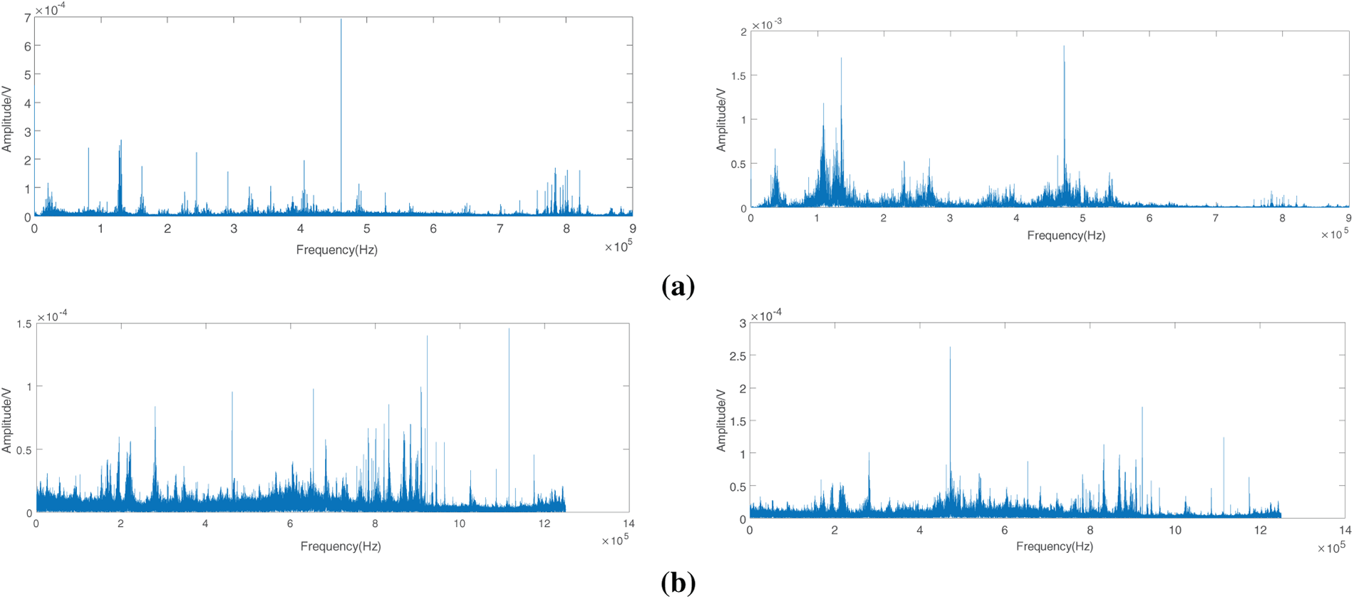
Figure 5: Frequency domain diagram after wavelet decomposition and reconstruction of leakage signals and non-leakage signals. (a) Spectrum diagram after reconstruction of approximate coefficient; (b) Spectrum diagram after reconstruction of detail coefficient.

By comparing the approximation-coefficient spectra of the non-leakage signal and the leakage signal, it can be observed that, in the non-leakage condition, the spectrum within 0–400 kHz exhibits only a few isolated peaks caused by environmental noise, and no obvious continuous peaks are present. After leakage occurs, this frequency band undergoes significant changes: distinct peaks appear between 50 and 300 kHz, while the other frequency regions remain almost unchanged, which is consistent with the analysis in Section 3.2. A comparison of Fig. 6 shows that the spectra of the detail coefficients exhibit no substantial differences between the non-leakage and leakage conditions, indicating that, after wavelet decomposition, most of the useful leakage-related information resides in the approximation coefficients, whereas the detail coefficients contain more noise components. Moreover, the differences between the non-leakage and leakage signals in the reconstructed spectra after wavelet decomposition are more pronounced than those observed in the original, unprocessed spectra. This demonstrates that wavelet analysis not only filters out a large portion of the environmental noise but also preserves more useful information in the approximation part of the signal.

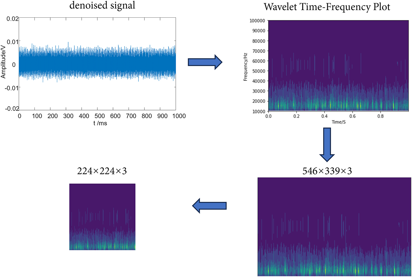
Figure 6: Time-frequency map construction process.

From the above analysis, it can be concluded that a large amount of noise is present in the acquisition environment. Due to the high sensitivity of the AE sensor, non-stationary environmental vibrations are recorded even under non-leakage conditions. Frequency-spectrum analysis shows that the leakage-related energy is mainly concentrated in the 50–300 kHz band.

To obtain effective leakage information, the AE signals were subjected to multiscale wavelet decomposition and reconstruction. Comparison of the spectra of the reconstructed signals at different scales indicates that the approximation coefficients retain most of the leakage-related components, whereas the detail coefficients are dominated by noise. Denoising based on the approximation coefficients enhances the separability between leakage and non-leakage conditions, thereby improving the overall performance of leakage state recognition.

4  Data Processing

4.1 Dataset Construction

The input of the model consists of time–frequency maps, which serve as the network input features. The construction process of these maps is illustrated in Fig. 6. First, for each leakage condition, 50 raw signal files (each with a duration of 10 s) were collected. These 50 raw files were randomly divided into two independent groups: a Training Source Set (35 files) and a Testing Source Set (15 files). To suppress environmental interference and enhance feature clarity, the raw signals in both sets were processed using the wavelet denoising and reconstruction method described in Section 3.3. Subsequently, a data augmentation strategy using sliding window slicing was applied independently to these two groups. Due to the sampling frequency of 2.5 MHz, a 0.1 s window size was selected to capture the complete periodic characteristics of AE signals in the frequency range of 50–300 kHz and balance sample generation efficiency. The sliding window moved across the raw signals with an overlap to generate sufficient samples. Ultimately, 700 samples were generated from the Training Source Set and 300 samples from the Testing Source Set for each condition, resulting in a total of 1000 samples per condition. The original size of each time-frequency diagram is 546 × 339 × 3. Before being fed into the network, axis labels and blank borders were removed, and images were resized to 224 × 224 × 3.

After applying CWT to denoise AE signals with varying leakage rates and converting them into time-frequency maps, the results are shown in Fig. 7.

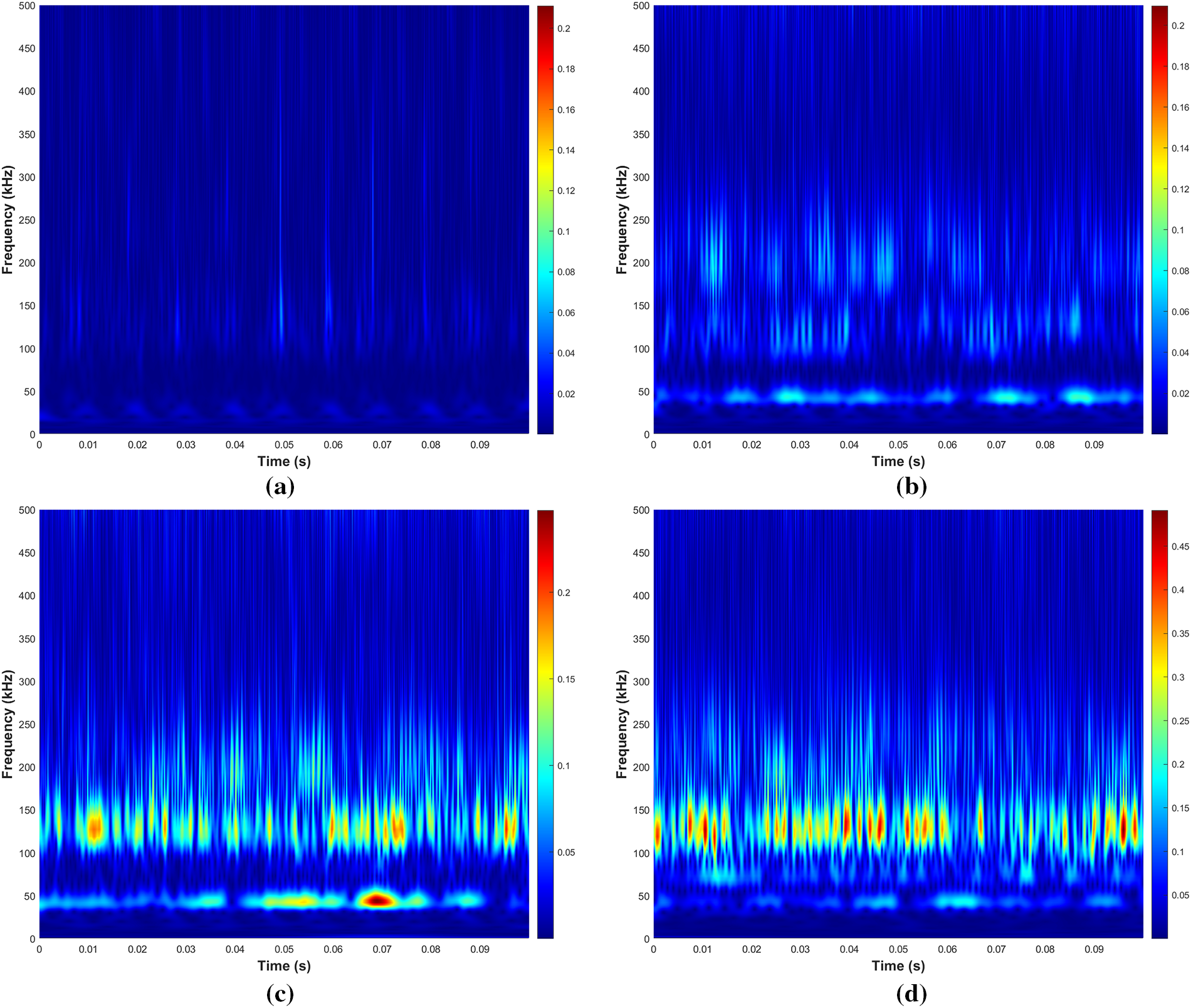
Figure 7: Wavelet time-frequency maps at different leakage rates. (a) 0 mL/min; (b) 200 mL/min; (c) 400 mL/min; (d) 600 mL/min.

As shown in Fig. 7, the time-frequency maps depicts time on the horizontal axis and frequency on the vertical axis, with color intensity representing signal amplitude. Comparing plots under different leakage rates reveals that at zero leakage (0 mL/min), energy distribution is relatively dispersed with low amplitude. At low leakage (200 mL/min), energy noticeably concentrates in the 50–150 kHz subband. For large leaks (400 & 600 mL/min), energy further intensifies within the 150–300 kHz range and exhibits persistent longitudinal stripe textures, corresponding to steady-state turbulent noise induced by the leak. These quantifiable characteristics—including the energy ratio between specific sub-bands (e.g., 50–150 kHz and 150–300 kHz) and the texture continuity index—serve as the key discriminative criteria automatically learned by the deep learning model employed in this paper to distinguish different leakage states.

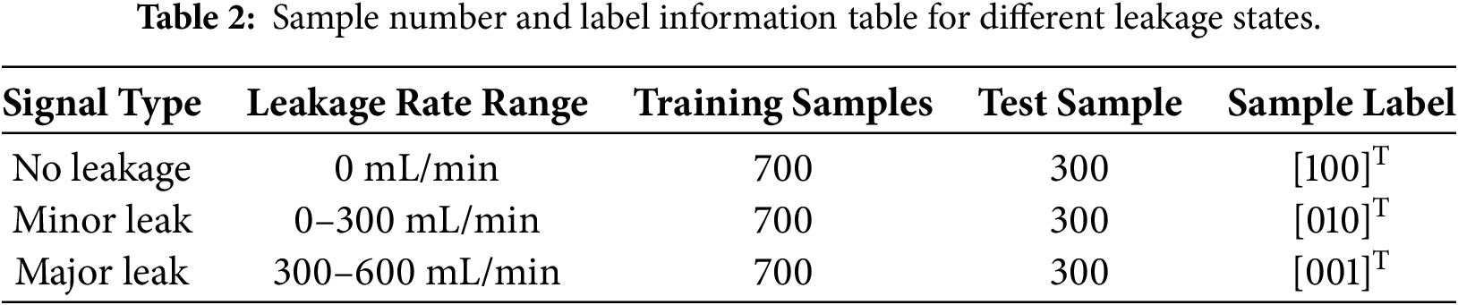
After constructing the wavelet time-frequency maps, the images were categorized according to leakage conditions. The dataset was divided into training and testing samples, and each sample was assigned a corresponding label using one-hot encoding. The dataset partitioning and label assignments for different pipeline leakage conditions are summarized in Table 2.

4.2 Network Architecture Design

The pipeline leakage state recognition model based on Inception-V3 is illustrated in Fig. 8. The Inception-V3 architecture was imported from TensorFlow, and the network weights were initialized using ImageNet pre-trained parameters. A Dense layer with 1024 neurons was first added, using the ReLU activation function. To prevent overfitting, a Dropout layer [18] and a Batch Normalization (BN) layer were introduced after the Dense layer. Subsequently, another Dense layer with 512 neurons and an additional BN layer were added. Finally, a Dense layer with 3 neurons followed by a Softmax classifier was employed to perform the three-category classification of pipeline leakage states. The adaptive moment estimation (Adam) optimizer was used for model training, and the Cross-Entropy Loss function was adopted as the loss criterion.

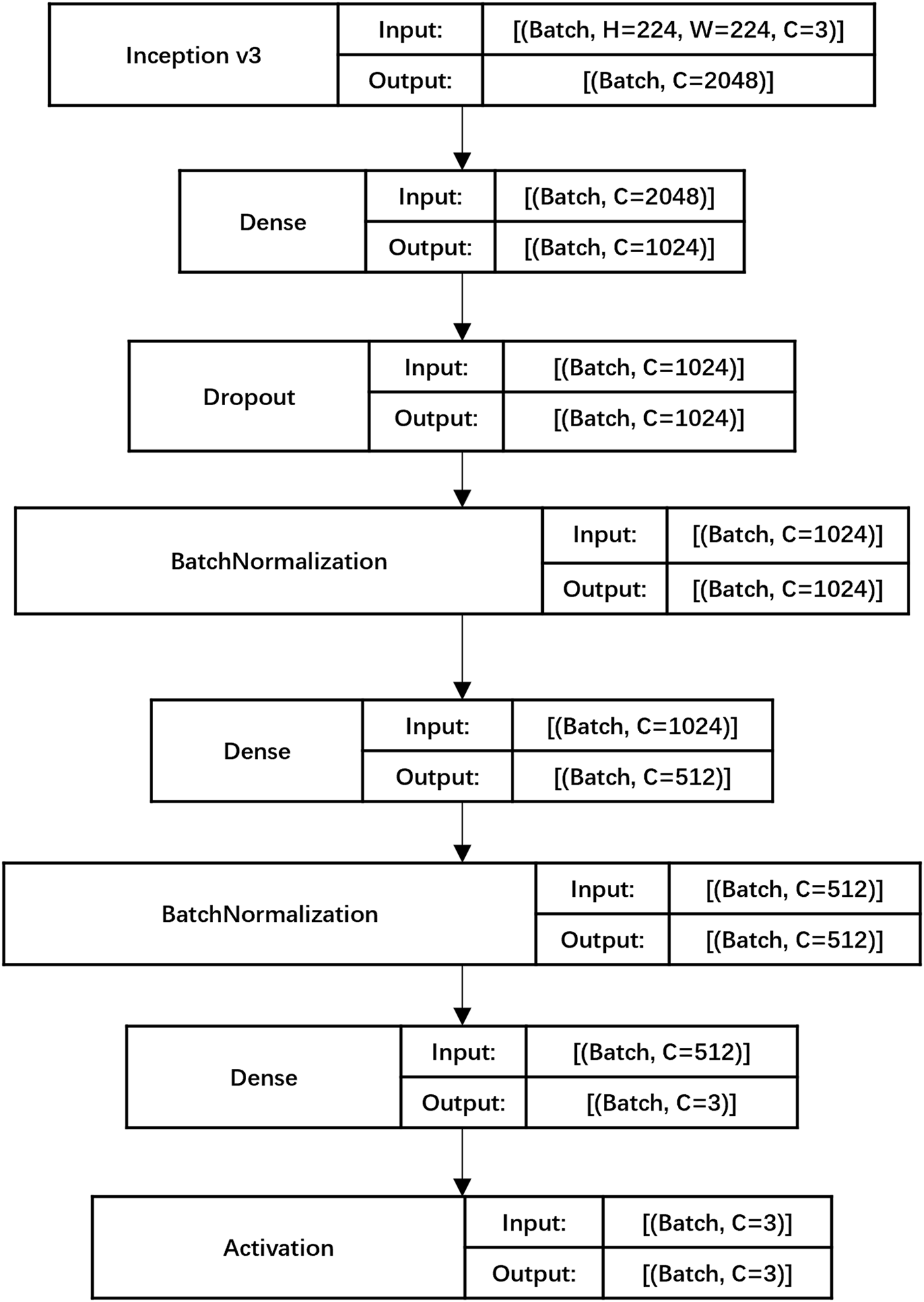
Figure 8: Network structure diagram.

4.3 Experimental Results and Analysis

The training time and accuracy of the network are influenced by the learning rate, number of epochs, and batch size. To achieve optimal classification performance, different combinations of these parameters were tested. The learning rate was fixed at 0.01, while the number of epochs and batch size were varied. The corresponding test set accuracies under different parameter configurations are summarized in Table 3.

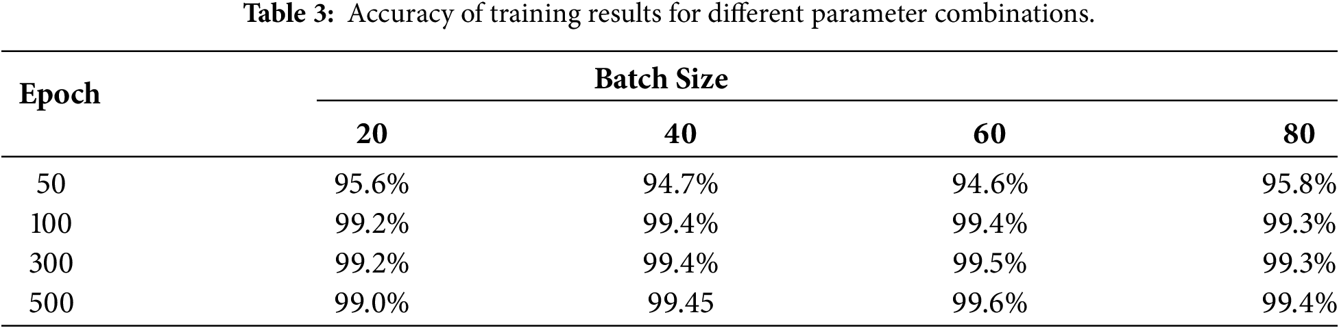
As shown in Table 3, when the number of epochs exceeds 50, the training results remain stable and satisfactory. When the learning rate is set to 0.01, the epoch to 500, and the batch size to 60, the model achieves the highest accuracy of 99.6%. Keeping the number of epochs fixed at 500 and the batch size at 60, the learning rate was then varied, and the corresponding training results are presented in Table 4.

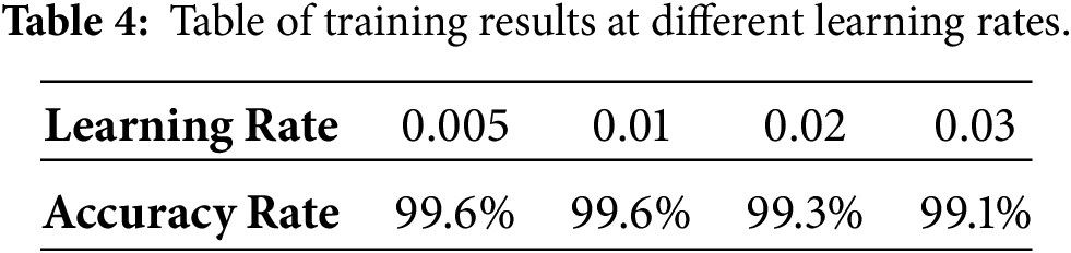
As shown in Table 4, when the learning rate is set to 0.005 or 0.01, the network achieves the highest accuracy of 99.6%. However, when the learning rate is 0.005, the overall training time is significantly longer. Therefore, the final training configuration is as shown in Table 5. The training and testing set loss values and accuracy rates are shown in Fig. 9.

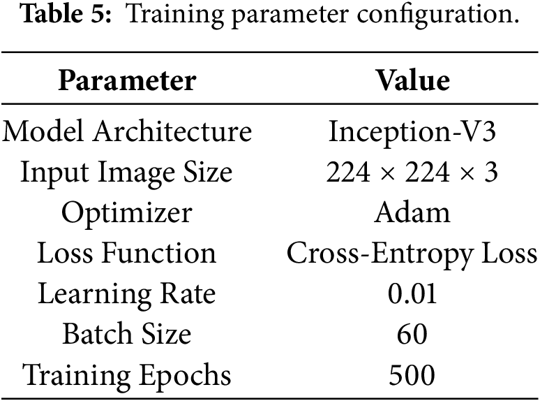
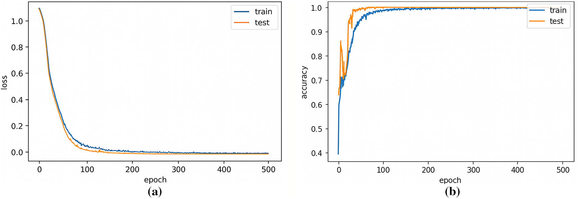
Figure 9: Training results. (a) Loss; (b) Accuracy rate.

From the loss curve of the model, it can be observed that after 500 training epochs, both the training and testing loss values approach zero, indicating that the model converges well without overfitting. As shown in Fig. 9, the final classification accuracy stabilizes at 99.6%, demonstrating that the model constructed using wavelet time-frequency maps and the Inception-V3 network can successfully identify the leakage states of the pipeline. On standard GPU platforms, the Inception-V3 model has a single sample inference time of only 21 ms. This confirms that the method is computationally efficient and fully meets the requirements of real-time industrial leak monitoring.

To validate the classification superiority of the Inception V3 network utilizing wavelet time-frequency maps as inputs, this study compared the accuracy of various deep learning models against a detection model based on feature parameters and SVM. As illustrated in Fig. 10a, the results demonstrate that deep learning models employing wavelet time-frequency maps generally achieve higher recognition accuracy than the SVM model based on feature parameters. Furthermore, among the deep learning models compared, the Inception V3 model exhibits the highest accuracy and stability, indicating superior overall performance.

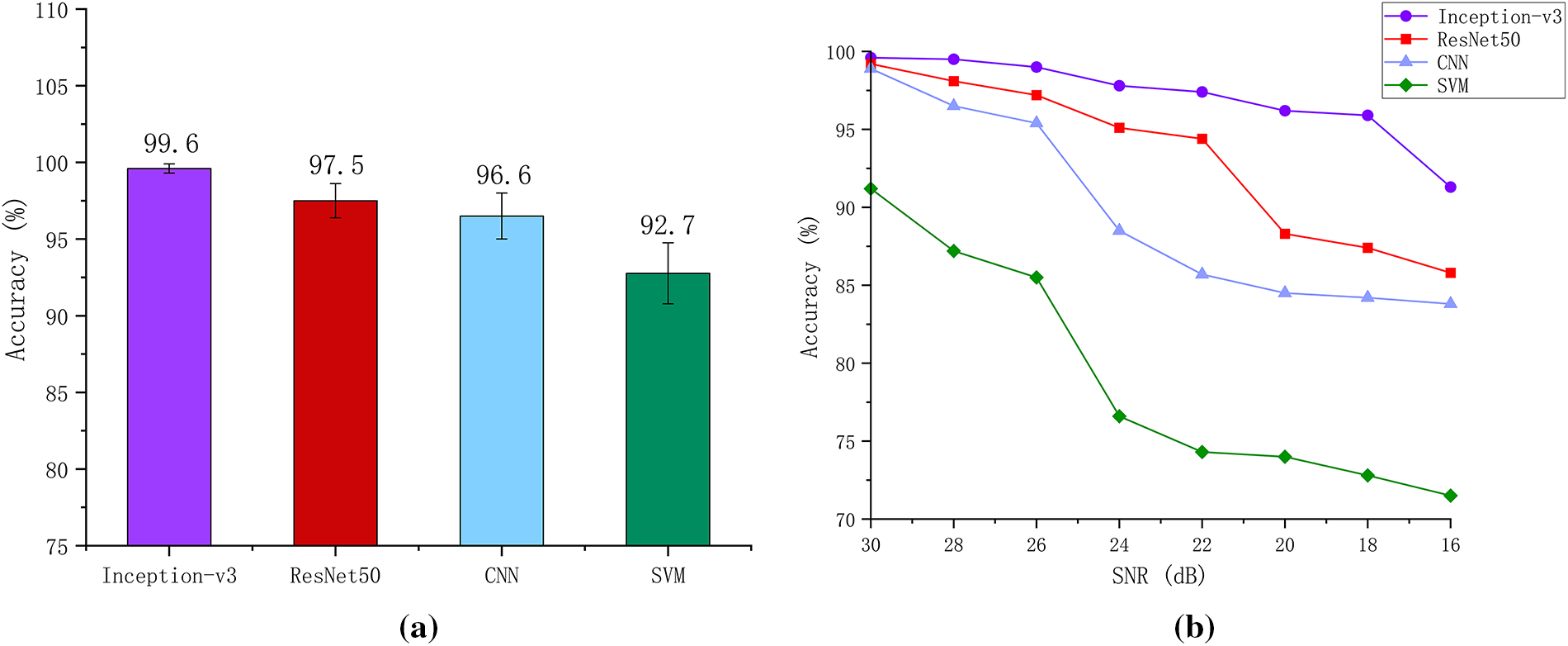
Figure 10: Average accuracy rate from multiple trials under various operating conditions. (a) Comparison across different models; (b) Performance comparison after adding gaussian white noise.

Additionally, considering the prevalence of noise interference in real-world environments, the recognition accuracy and robustness of the neural network models were examined by injecting Gaussian white noise into the original dataset to generate varying SNRs. Specifically, noise levels corresponding to SNRs of 30, 28, 26, 24, 22, 20, 18, and 16 dB were introduced to evaluate stability. The mean accuracy and error intervals were calculated, as presented in Fig. 10b. While the introduction of noise inevitably degrades model accuracy—particularly under low SNR conditions—the Inception V3 model only exhibits a significant decline when the SNR drops to 16 dB, maintaining stability at SNRs above 16 dB. In contrast, other methods experience accuracy degradation at higher SNRs (e.g., 26 and 22 dB). Consequently, it can be concluded that the Inception V3 model based on wavelet time-frequency maps possesses excellent robustness and stability.

For certain critical components in industrial equipment, any micro-leakage must be detected as quickly as possible. To achieve this, leakage states are further subdivided, as shown in Table 6. Data is collected to build an image-based dataset, and the Inception-V3 model is used to identify the refined leakage categories. The confusion matrix for the classification results is shown in Fig. 11.

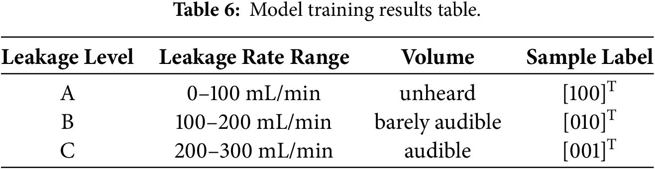
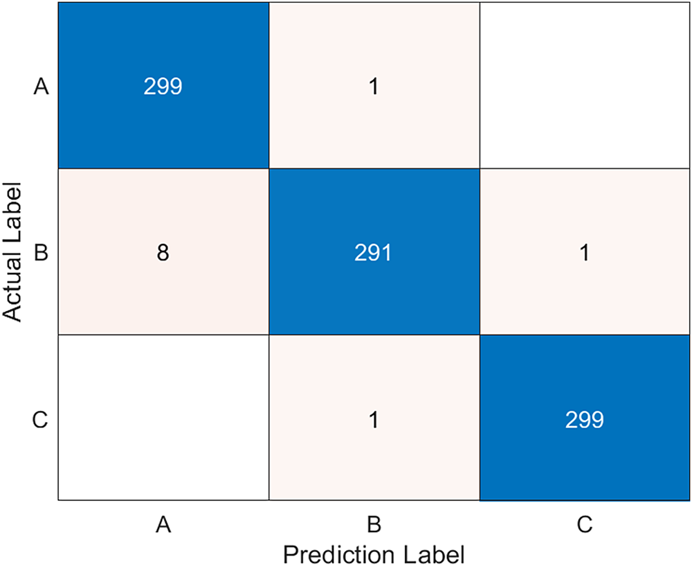
Figure 11: Leak classification confusion matrix.

As observed from the classification confusion matrix, the proposed method achieves a remarkably high accuracy of 98.8%, even under micro-leakage conditions. Specifically, the recognition accuracy is notably high for true leakage levels corresponding to Level A and Level C. Furthermore, misclassifications are restricted to adjacent categories—with no cross-category errors occurring—indicating an ideal prediction performance. The majority of misjudgments are concentrated in Level B, where 8 samples were misclassified as Level A. This is primarily attributed to the high similarity of acoustic features generated at leakage rates near the class boundaries, particularly when the leakage rate is low, which results in increased difficulty in differentiation.

5  Conclusion

To address the issue of pipeline leakage detection, a pipeline leakage experimental platform was established based on an RS-2A AE sensor. Three different leakage conditions were simulated, and the corresponding AE signals were collected and analyzed. The acquired signals were analyzed using MATLAB, and the results indicated that the leakage signals were mainly distributed within the 50–300 kHz frequency band. Wavelet decomposition and reconstruction were then applied to perform denoising pre-processing of the signals. To achieve accurate leakage state identification under complex working conditions, the CWT was employed to convert the signals into wavelet time-frequency maps. A pipeline leakage recognition model was then constructed based on the Inception-V3 network, achieving a recognition accuracy of 99.6%. Through a comparative analysis with alternative deep learning architectures and feature-based SVM models, the proposed Inception V3 framework—utilizing wavelet time-frequency maps—demonstrated superior accuracy and enhanced robustness, particularly in high-noise environments. Notably, high precision was maintained even under micro-leakage conditions. These results substantiate the efficacy and reliability of the proposed method for pipeline leak detection.

Acknowledgement: The author extends their sincere gratitude and appreciation to the School of Mechanical and Power Engineering, East China University of Science and Technology and the School of Artificial Intelligence, Shenzhen Technology University.

Funding Statement: This research was supported by the National Key R&D Program of China (2023YFC3010500).

Author Contributions: The authors confirm contribution to the paper as follows: conceptualization, Siqiang Zheng, Xuetong Xu and Yu Lu; methodology, Siqiang Zheng, Xuetong Xu and Yu Lu; software, Siqiang Zheng and Xuetong Xu; validation, Siqiang Zheng, Lanzhu Zhang, Yu Lu and Zhiqin Qian; formal analysis, Siqiang Zheng, Xuetong Xu and Kai Sun; investigation, Siqiang Zheng, Xuetong Xu and Kai Sun; resources, Lanzhu Zhang and Zhiqin Qian; data curation, Siqiang Zheng and Xuetong Xu; writing—original draft preparation, Siqiang Zheng and Lanzhu Zhang; writing—review and editing, Siqiang Zheng, Lanzhu Zhang and Zhiqin Qian; visualization, Siqiang Zheng; supervision, Lanzhu Zhang and Zhiqin Qian; project administration, Lanzhu Zhang and Zhiqin Qian; funding acquisition, Lanzhu Zhang and Zhiqin Qian. All authors reviewed and approved the final version of the manuscript.

Availability of Data and Materials: The datasets generated during and analyzed during the current study are available from the corresponding authors on reasonable request.

Ethics Approval: Not applicable.

Conflicts of Interest: The authors declare no conflicts of interest.

References

1. Galiatsatos N, Kousiopoulos GP, Petsa A, Kampelopoulos D, Giannopoulos F, Spandonidis C, et al. Industrial Internet of Things platform for leak detection and localization in oil and gas pipelines. In: Proceedings of the 6th Smart Cities Symposium (SCS 2022); 2022 Dec 6–8; Online. p. 296–300. doi:10.1049/icp.2023.0535. [Google Scholar] [CrossRef]

2. Wu H, Jiang Z, Zhang X, Cheng J. Research on a novel unsupervised-learning-based pipeline leak detection method based on temporal Kolmogorov-Arnold network with autoencoder integration. Sensors. 2025;25(2):384. doi:10.3390/s25020384. [Google Scholar] [PubMed] [CrossRef]

3. Zhang Z, Xu C, Xie J, Zhang Y, Liu P, Liu Z. MFCC-LSTM framework for leak detection and leak size identification in gas-liquid two-phase flow pipelines based on acoustic emission. Measurement. 2023;219:113238. doi:10.1016/j.measurement.2023.113238. [Google Scholar] [CrossRef]

4. Wang L, Gao Y, Li X, Gao L. Self-supervised-enabled open-set cross-domain fault diagnosis method for rotating machinery. IEEE Trans Ind Inform. 2024;20(8):10314–24. doi:10.1109/TII.2024.3396335. [Google Scholar] [CrossRef]

5. An G, Huang Z, Li Y. Constant false alarm rate detection of pipeline leakage based on acoustic sensors. Sci Rep. 2023;13(1):14149. doi:10.1038/s41598-023-41177-3. [Google Scholar] [PubMed] [CrossRef]

6. Dao F, Zeng Y, Qian J. Fault diagnosis of hydro-turbine via the incorporation of Bayesian algorithm optimized CNN-LSTM neural network. Energy. 2024;290:130326. doi:10.1016/j.energy.2024.130326. [Google Scholar] [CrossRef]

7. Huang Y, Tao J, Sun G, Wu T, Yu L, Zhao X. A novel digital twin approach based on deep multimodal information fusion for aero-engine fault diagnosis. Energy. 2023;270:126894. doi:10.1016/j.energy.2023.126894. [Google Scholar] [CrossRef]

8. Zhang B, Yuan H, Ge J, Cheng L, Li X, Xiao C. Weak appearance aware pipeline leak detection based on CNN-transformer hybrid architecture. IEEE Trans Instrum Meas. 2025;74:5002009. doi:10.1109/TIM.2024.3504562. [Google Scholar] [CrossRef]

9. Ullah S, Ullah N, Siddique MF, Ahmad Z, Kim JM. Spatio-temporal feature extraction for pipeline leak detection in smart cities using acoustic emission signals: a one-dimensional hybrid convolutional neural network-long short-term memory approach. Appl Sci. 2024;14(22):10339. doi:10.3390/app142210339. [Google Scholar] [CrossRef]

10. Yu Y, Li Y, Yang P, Pu F, Ben Y. TFC-TFECR feature extraction and state recognition of acoustic emission signal of cylindrical roller bearing. Nondestruct Test Eval. 2025;40(3):1034–52. doi:10.1080/10589759.2024.2338480. [Google Scholar] [CrossRef]

11. Naseem S, Mahmood T, Khan AR, Farooq U, Nawazish S, Alamri FS, et al. Image fusion using wavelet transformation and XGboost algorithm. Comput Mater Contin. 2024;79(1):801–17. doi:10.32604/cmc.2024.047623. [Google Scholar] [CrossRef]

12. Saleem F, Ahmad Z, Kim JM. Real-time pipeline leak detection: a hybrid deep learning approach using acoustic emission signals. Appl Sci. 2024;15(1):185. doi:10.3390/app15010185. [Google Scholar] [CrossRef]

13. Siddique MF, Ahmad Z, Ullah N, Kim J. A hybrid deep learning approach: integrating short-time Fourier transform and continuous wavelet transform for improved pipeline leak detection. Sensors. 2023;23(19):8079. doi:10.3390/s23198079. [Google Scholar] [PubMed] [CrossRef]

14. Song L, Cui X, Han X, Gao Y, Liu F, Yu Y, et al. A non-metallic pipeline leak size recognition method based on CWT acoustic image transformation and CNN. Appl Acoust. 2024;225(8):110180. doi:10.1016/j.apacoust.2024.110180. [Google Scholar] [CrossRef]

15. Siddique M, Ahmad Z, Ullah N, Ullah S, Kim J. Pipeline leak detection: a comprehensive deep learning model using CWT image analysis and an optimized DBN-GA-LSSVM framework. Sensors. 2024;24(12):4009. doi:10.3390/s24124009. [Google Scholar] [PubMed] [CrossRef]

16. Sahoo GR, Freed JH, Srivastava M. Optimal wavelet selection for signal denoising. IEEE Access. 2024;12:45369–80. doi:10.1109/access.2024.3377664. [Google Scholar] [PubMed] [CrossRef]

17. Wang L, Zheng W, Ma X, Lin S. Denoising speech based on deep learning and wavelet decomposition. Sci Program. 2021;2021(1):8677043. doi:10.1155/2021/8677043. [Google Scholar] [CrossRef]

18. Zhang Z, Xu ZJ. Implicit regularization of dropout. IEEE Trans Pattern Anal Mach Intell. 2024;46(6):4206–17. doi:10.1109/TPAMI.2024.3357172. [Google Scholar] [PubMed] [CrossRef]