
 Submit a Paper
 Propose a Special lssue
 Open Access
ARTICLE

Context-Adaptive and Physics-Consistent Constrained Multimodal Interpretable Remaining Useful Life Prediction
1 Department of Command and Management, Shijiazhuang Campus, Army Engineering University of PLA, Shijiazhuang, China
2 Hebei Provincial Key Laboratory of Condition Monitoring and Evaluation of Machinery and Equipment, Hebei Provincial Department of Science and Technology, Shijiazhuang, China
* Corresponding Author: Zhonghua Cheng. Email:
Computers, Materials & Continua 2026, 87(3), 77 https://doi.org/10.32604/cmc.2026.077026
Received 01 December 2025; Accepted 13 February 2026; Issue published 09 April 2026
 View Full Text
 Download PDF
Abstract
Remaining useful life (RUL) prediction for complex equipment is a critical technology for ensuring the safe and reliable operation of industrial systems. However, existing data-driven models commonly suffer from limitations such as weak cross-operational condition generalization, insufficient physical interpretability, and unstable training on non-stationary time-series data. To address these challenges, this paper proposes a temporal degradation prediction model that integrates context adaptation and physics-consistent constraints, named the Context-Adaptive Physics-informed Time-aware meta-Network (CAPTAIN). The model incorporates four core components: a Context-Aware Meta-Learning (CAML) module that enables lightweight parameter adaptation to diverse scenarios; Physics-Informed Neural Network (PINN) constraints that uniformly characterize deterministic degradation dynamics and stochastic Wiener process perturbations; a three-layer dynamic stabilization training strategy comprising temporal meta-training, residual adaptive refinement, and exponential moving average to ensure training stability; and a multimodal interpretability framework integrating LIME, GradCAM, GradCAM_LW, Integrated Gradients, and KernelSHAP to enhance prediction transparency. Extensive experiments on the NASA C-MAPSS datasets (FD001–FD004) demonstrate that CAPTAIN achieves state-of-the-art performance under both single/multiple failure modes and steady/varying operating conditions, with an average RMSE of 12.02 ± 0.98 and an average SCORE of 487.50 ± 23.0, outperforming ten advanced baseline models. The model exhibits exceptional generalization capability across different operational conditions and strong robustness in scenarios with coupled multiple faults. Multimodal visualizations and quantitative assessments verify its interpretability advantages, showing high consistency with the physical degradation laws of engines. This work provides a reliable paradigm for RUL prediction of complex equipment, combining the flexibility of data-driven modeling with the credibility of physical modeling.Keywords
With the rapid advancement of industrial intelligence, Prognostics and Health Management (PHM) has become a core technology for ensuring the safe and reliable operation of complex equipment and reducing maintenance costs. As a key component of PHM, Remaining Useful Life (RUL) prediction directly affects the scientific validity and timeliness of maintenance decisions, holding indispensable engineering value in critical fields such as aerospace, new energy, and nuclear power. Taking aircraft engines as an example, their complex and variable operating environments, highly nonlinear degradation processes, and coupled multiple failure modes impose stringent requirements on the accuracy, generalization capability, and physical consistency of RUL prediction models [1].
Existing RUL prediction methods can be broadly categorized into data-driven, physics-model-driven, and hybrid-driven approaches, yet each exhibits notable limitations. Traditional data-driven methods (e.g., CNN, LSTM) can capture temporal features but heavily rely on large amounts of labeled data and show weak generalization across multiple operating conditions and fault scenarios. Meta-learning and adaptive models (e.g., Meta-LSTM, Transformer variants) attempt to improve cross-scenario adaptability, but their parameter adjustment mechanisms are often simplistic, struggling to balance computational cost and adaptation range. Physics-model-driven methods, grounded in explicit degradation mechanisms, offer strong interpretability; however, they face high modeling complexity and poor noise resistance when dealing with the nonlinear degradation processes of complex equipment. Hybrid-driven methods, particularly Physics-Informed Neural Networks (PINN), seek to combine the strengths of both, yet most current studies adopt simplistic physical constraint embedding, failing to achieve deep integration of data features and physical laws. They also exhibit significant shortcomings in uncertainty quantification and adaptability to multi-failure scenarios. Moreover, most intelligent prediction models remain “black boxes,” whose lack of interpretability hinders trust from engineering practitioners, limiting their practical deployment in critical industrial applications [2].
To address these issues, this paper proposes a temporal degradation prediction model named CAPTAIN (Context-Adaptive Physics-informed Time-aware meta-Network), which integrates physics-consistent constraints and context adaptation. The core innovations of the model include four aspects: first, the design of a Context-Aware Meta-Learning (CAML) module that enables lightweight parameter adaptation to enhance generalization across varying conditions; second, the construction of a physics-constrained loss that integrates state-dependent dynamics and a Wiener stochastic process to ensure the physical consistency of predictions; third, the proposal of a three-layer dynamic stabilization training strategy comprising Sequential Meta-Training (SMT), Residual-based Adaptive Refinement (RAR), and Exponential Moving Average (EMA) to enhance training stability; and fourth, the integration of a multimodal interpretability framework (including Grad-CAM, LIME, SHAP, etc.) to improve the transparency and engineering credibility of the predictions.
Experimental results based on the NASA C-MAPSS benchmark dataset demonstrate that the CAPTAIN model achieves excellent performance under both multiple operating conditions and multiple fault scenarios, with average RMSE and SCORE metrics surpassing those of existing advanced methods. The main contributions of this paper are as follows:
(1) Proposal of a data- and physics-dual-driven adaptive fusion framework that balances operational condition adaptability and physical consistency;
(2) Development of a systematic dynamic stabilization training mechanism that significantly enhances model robustness and generalization capability;
(3) Establishment of a multi-dimensional interpretability system that aligns prediction results with physical meaning.
The remainder of this paper is organized as follows: Section 2 reviews related research work; Section 3 details the architecture design and training mechanism of the CAPTAIN model; Section 4 describes the experimental design, dataset preprocessing, and evaluation metrics, followed by analysis of the results and validation of the model’s effectiveness; Section 5 concludes the paper and outlines future research directions.
2.1 Temporal Data-Driven RUL Prediction Models
Temporal data-driven models are central to RUL prediction. Compared to traditional statistical methods (e.g., HMM, regression) that suffer from poor generalization, deep models like CNNs, LSTMs, and GRUs offer superior feature extraction. For instance, Sharma et al. [3] combined 1D-CNN attention with GRU for turbofan engines; however, fixed parameters and sensitivity to condition variations limit their multi-scenario efficacy.
To improve feature representation, GNNs and multi-modal fusion have emerged. Xiao et al. [4] used HGCN-CIP with heterogeneous graphs to model sensor interactions, though cross-window context and long-term degradation remain under-exploited. Xu et al. [5] developed STDD-Net, integrating CEEMD and capsule networks for pattern disentanglement, albeit with high computational costs. In battery applications, Chen et al. [6] employed a CNN-PCC extractor for joint SOH–RUL prediction but required complete charging records. Wang et al. [7] fused impedance features with ResMLP and TCN-Attention to avoid heavy computation, yet relied on specialized measurements. Rengarajan and Anuradha [8] combined TFT and ND-RNN with the Vulture Optimization Algorithm, though the high parameter count hinders real-time deployment.
Meta-learning and adaptive frameworks further address cross-condition and few-shot challenges. Wang et al. [9] proposed MKDPINN, using physics-guided regulators and meta-learning for domain transfer, but lacked fine-grained parameter-level adaptation. Zheng et al. [10] utilized Meta-LSTM to model stochastic degradation, neglecting sample-level context. Hu et al. [11] introduced DSCN-AttnPINN for enhanced feature extraction, yet remained dependent on preprocessing. Lastly, Jiang et al. [12] used an improved Transformer with window fusion to capture cross-phase dependencies, though fixed rules struggle with diverse degradation rhythms. Despite progress, current models lack lightweight parameter-level adaptivity and multi-scale temporal modeling. Their loose integration with meta-learning continues to limit generalization under complex, few-shot scenarios.
2.2 Physics-Informed Fusion Prediction Methods
Physics-informed fusion methods integrate domain knowledge with data features to balance accuracy and physical consistency. PINNs, as a core framework, embed physical equations into loss functions to enhance interpretability. For example, Li et al. [13] proposed a lightweight BiMamba-PINN for efficient long-sequence modeling, but it relies on simple equations and struggles with stochastic degradation under noise. Hu et al. [14] combined residual connections with DeepHPM for SOH and RUL prediction, yet their battery-specific constraints lack cross-equipment generality. Similarly, Wang et al. [15] embedded reliability knowledge and Weibull distributions into a PINN for bearing RUL, but assumed a single failure mode. Kim et al. [16] fused Weibull and Arrhenius-based models using a composite loss, though the physical and data-driven components were only loosely coupled.
Recent improvements focus on constraint forms and uncertainty quantification. Xie et al. [17] introduced BPINN with iterative Ensemble Kalman Inversion for joint RUL and uncertainty estimation; however, fixed loss weights often lead to over-constraint or data-dominance. Dersin and Rocchetta [18] linearized Mean Residual Life for explicit confidence intervals but relied on specific distributions (e.g., Weibull), limiting flexibility. Ma et al. [19] utilized charging-time and voltage-plateau parameters to reduce data dependence, but performance drops significantly with missing data or charging interruptions.
Beyond PINNs, hybrid fusion strategies offer alternative paths. Wang et al. [7] integrated impedance-derived features with ResMLP and TCN-Attention to improve interpretability, though real-time acquisition of impedance data remains difficult. Overall, current physics-informed methods are hindered by fixed-form constraints, non-adaptive loss balancing, and high-cost uncertainty quantification, limiting their robustness in complex, stochastic degradation processes.
2.3 Generalization, Optimization, and Interpretability of RUL Models
Generalization and interpretability are vital for practical RUL deployment, yet current research faces significant limitations. While Chen et al. [6] and Rengarajan and Anuradha [8] improved generalization via expert-based preprocessing and heuristic hyperparameter tuning, their methods remain device-specific or computationally expensive. Similarly, XAI applications by Sharma et al. [3] (LIME) and Yuktha and Manimaran [2] (SHAP) provide feature-level insights but lack physical consistency and stage-wise clarity. These gaps manifest as a persistent struggle to balance multi-condition adaptability with physical constraints, a lack of stabilization mechanisms for non-stationary temporal data, and a reliance on singular interpretability frameworks that decouple data-driven results from physical degradation laws. To bridge these gaps, the proposed CAPTAIN model integrates a CAML–physics coupled architecture for joint adaptation and consistency, employs a three-layer dynamic stabilization strategy (SMT + RAR + EMA) tailored for non-stationary degradation, and implements a multimodal interpretability framework with seven metrics to achieve “local–global–physical” explanations aligned with equipment degradation mechanisms.
This paper proposes the Context-Adaptive Physics-informed Time-aware meta-Network (CAPTAIN), a temporal degradation prediction model that seamlessly integrates physics-consistent constraints with context adaptation. Its objective is to learn a mapping function through the following core components:
here, x ∈ RT×F represents a sensor time-series segment, t ∈ [0, 1] is the normalized time variable, and
The model architecture, illustrated in Fig. 1, integrates a data encoder, a context adaptation module, a physics-constrained head, and a dynamic stabilization training mechanism. The overall workflow can be divided into three stages: (1) Feature Encoding and Contextual Adaptation, (2) Physics-Consistent Prediction and Constraint Calculation, and (3) Dynamic Stabilization Optimization (SMT + RAR + EMA).

Figure 1: CAPTAIN overall structure and information flow.
3.1 Context Attention and Parameter Lightweight Adaptation Mechanism
Conventional PINN or RUL prediction models often rely on fixed parameters and are highly sensitive to varying operational conditions, thereby struggling to achieve sample-level generalization, as shown in Fig. 2. To address this limitation, the CAPTAIN model incorporates a CAML module, which performs adaptive adjustment based on the contextual information of samples from different time windows. Let the input sequence be denoted as x = [x1, …, xT]. The CAML module first generates temporal attention weights as follows:
where
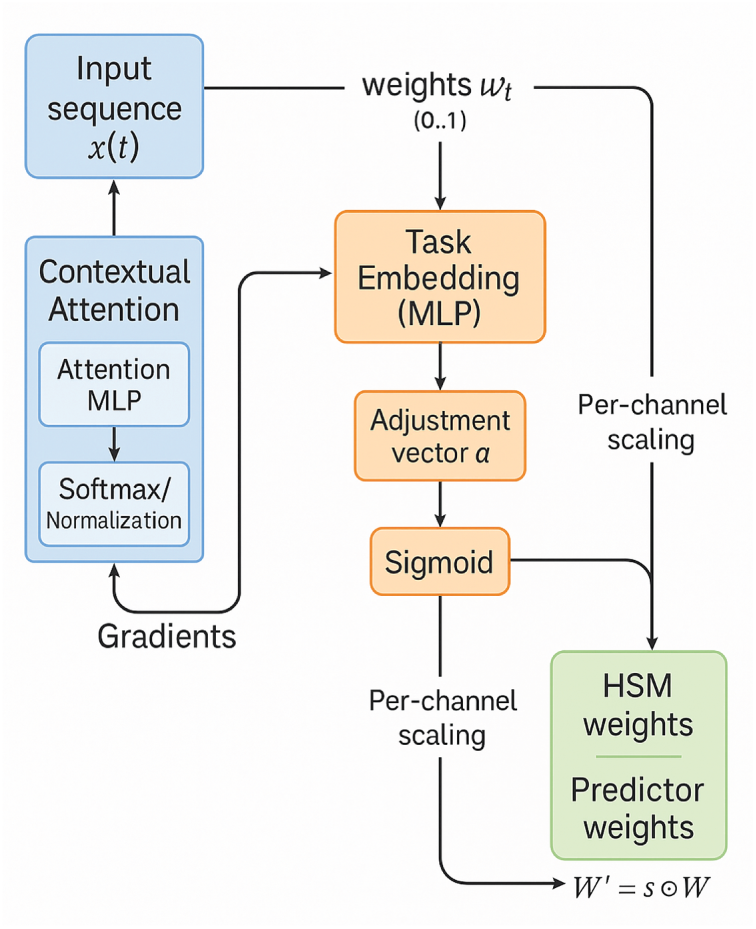
Figure 2: CAML module structure and parameter adjustment mechanism.
And normalize to get the context vector:
where
Through the task embedding mapping ϕ: RF → Rd, the adaptive adjustment vector a = ϕ(c) is generated, and the scaling factor is obtained by Sigmoid
This factor is applied to part of the parameter matrix, such as a convolutional or linear layer:
The subset of the parameter matrix (e.g., depthwise separable convolution kernels and linear prediction layers) is selected for scaling based on two primary criteria: (1) Sensitivity Criterion: priority is given to layers directly processing raw sensor feature maps, as they are most affected by operational fluctuations; (2) Computational Efficiency Criterion: by adjusting only approximately 5%–10% of the critical parameters, the model can achieve rapid task migration while maintaining low inference latency. Thus, the lightweight adaptive adjustment of parameters is realized in the stage of feature extraction and prediction.
This context-parameter coupling mechanism enables the model to migrate quickly under different working conditions. This is equivalent to adding a conditional modulation function to the original network fθ(x, t) as follows:
The gradient of s(c) can be learned directly via backpropagation.
Furthermore, the CAML mechanism exhibits high architectural scalability. In deeper or more complex networks (such as deep residual networks or Transformers), this mechanism can be seamlessly integrated into the scaling factors of residual connections or the projection matrices of self-attention mechanisms. Such a design not only enhances the cross-domain generalization capability of deep networks under multiple operating conditions but also effectively mitigates training instability issues common in meta-learning within deep structures.
3.2 Physics Consistency Constraints and PINN Loss Function
CAPTAIN treats the RUL prediction as a continuous-time degradation process
where k > 0 is the degradation coefficient, α ∈ [1, 2] controls the degree of nonlinearity of the degradation rate, and η(t) represents the noise disturbance term, and

Figure 3: Schematic representation of the physical meaning of PINN constraints with the residual path.
3.2.1 Deterministic Constraint Term
Compute the first and second derivatives of the model prediction
And construct three kinds of physical residuals:
The total residual is as follows.
where
In order to capture the operating fluctuations, the noise term based on Wiener process is constructed as follows.
where μ and σ are learnable drift and diffusion parameters.
Final combined residual:
Among them, the weight λ gradually decays to λmin with training, which enhances the randomness in the initial stage and strengthens the certainty in the later stage.
3.2.3 Loss Function Weighted with Uncertainty
The total loss uses a learnable log-variance trade-off mechanism:
The LIC initial value continuity term is used to keep the prediction of adjacent time Windows smoothly connected:
The loss function constructed above makes the model optimize the supervised error and the physical residual at the same time in the learning process, realizing the adaptive balance of data-physical dual driving.
3.3 Training Strategies for Dynamic Stabilization
To achieve convergence stabilization and cross-window generalization on non-stationary time series, CAPTAIN introduces a three-layer stabilization strategy, as shown in Fig. 4.

Figure 4: Dynamic stabilization training mechanism (SMT, RAR, EMA) process.
Firstly, SMT is used to divide the timeline into multiple Windows [tb, te], and each window trains independently and inherits the parameter snapshot θw−1 of the previous window, so as to achieve consistent parameter transfer across stages. The objective function for the current window is:
where
The regularization term ensures that the prediction behavior is continuous and stable in different stages.
Secondly, residual-based Adaptive Refinement (RAR) mechanism is used to randomly sample M time points {ti} in every few training steps, calculate the Residual modulus length ∣r(ti)∣, and select the maximum residual value t∗ = argmaxi∣r(ti)∣, and add the reinforcement term at this point:
where
This difficult-driven strategy can adaptively focus on physically inconsistent regions and improve the physical smoothness of boundary prediction and degradation turning points. Finally, the Exponential Moving Average (EMA) parameter smoothing strategy is used in training to maintain shaded variables for each parameter:
In the validation and testing phase, the parameter θ(EMA) is temporarily replaced to obtain smooth and stable performance. This three-layer mechanism forms a closed loop of sequential pass-hard focus-smooth evaluation during the optimization process, which enables the model to maintain stable training and cross-stage generalization under complex degradation curves.
This three-layer strategy not only theoretically achieves joint optimization across temporal and residual dimensions but also practically provides convergence stability similar to second-order optimization through parameter snapshot inheritance (SMT) and weight smoothing (EMA).
3.4 Mechanisms for Model Interpretability
To improve the transparency and diagnostics of the model in engineering applications, CAPTAIN integrates a multi-modal interpretable analysis framework, as shown in Fig. 5.
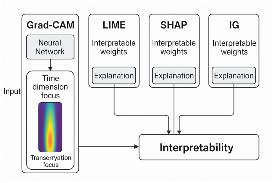
Figure 5: Mechanisms for multimode interpretability.
At the gradient level, a handwritten Grad-CAM mechanism is used to calculate the channel weights by capturing the convolutional layer feature map F with the gradient ∇Fy.
And generate a time heatmap:
Meanwhile, weighted Grad-CAM fuses multi-layer feature maps by weight ωl:
In addition, LIME, SHAP and IG interpreters are built-in in the model, which are used to analyze the feature importance from three perspectives of local linearity, global contribution and path integral. This multi-mode interpretation system forms a complementary structure of gradient saliency, local additivity and global fair decomposition, which makes the physical quantities output by the model traceable and interpretable.
To quantitatively evaluate the faithfulness of these explanations, we employ a refined Fidelity metric. Unlike traditional classification-based fidelity that uses zero-masking, we adopt a perturbation-based approach. This is crucial for physics-informed models like CAPTAIN, as zeroing out sensor values would violate the state-dependent dynamics equation, leading to numerical instability. By applying small Gaussian perturbations to identified ‘important’ features, we measure the sensitivity of the RUL prediction to ensure the explanations reflect the model’s true internal reasoning.
In summary, the proposed CAPTAIN framework integrates data-driven modeling and physics-based principles in a unified architecture and training scheme. CAML provides lightweight window-level context-aware parameter adaptation, while a PINN with state-dependent terms and a Wiener process jointly models deterministic and stochastic degradation, supported by an SMT–RAR–EMA strategy that stabilizes time-series meta-learning. Combined with a multimodal interpretability framework (Grad-CAM, LIME, SHAP, IG), CAPTAIN forms a physics-consistent, interpretable, and temporally stable RUL prediction paradigm with strong generalizability for complex equipment.
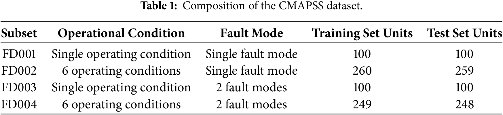
To validate the proposed CAPTAIN framework, we employed the Commercial Modular Aero-Propulsion System Simulation (C-MAPSS) dataset provided by NASA. This dataset is a widely adopted public benchmark in the PHM domain, comprising multiple sets of run-to-failure simulation data generated for turbofan engines via the C-MAPSS platform [20].
C-MAPSS is typically divided into four subsets (FD001–FD004), each corresponding to distinct operational condition combinations and fault modes. Each subset further consists of a training set and a test set. The training set records the complete life cycles of multiple engine units from initial operation to failure, while the test set provides observation sequences from another set of engines over specified operational intervals.
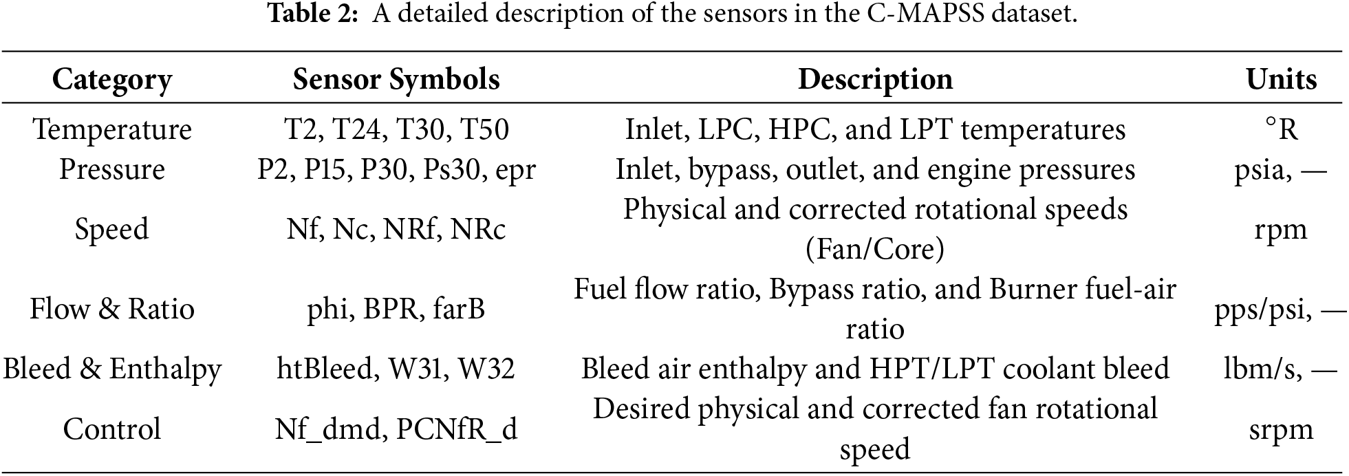
Each data sample includes the engine unit identifier, current flight cycle, three operational setting parameters, and readings from 21 sensors. These sensors are distributed across different components of the engine, monitoring critical variables such as temperature, pressure, and rotational speed, which collectively characterize the system’s health status. A summary of the dataset is provided in Table 1, and a detailed sensor list with descriptions is presented in Table 2.
4.2 Data Preprocessing and Training Configuration
Among 21 sensors in the C-MAPSS dataset, seven with constant readings were excluded to reduce complexity and focus on degradation information. The remaining 14 dynamic sensors (S2, S3, S4, S7, S8, S9, S11, S12, S13, S14, S15, S17, S20, S21) were selected for training. To mitigate operational condition interference, an operational-regime-based normalization method [21] was applied, followed by Locally Weighted Regression (LOESS) [22] to smooth time-series data and extract long-term degradation trends. The LOESS smoothing process employs a weighted least squares approach to minimize fitting errors within local neighborhoods.
Data were processed using a sliding-window strategy with a length of 15 and a step size of 1, resulting in (15, 14) sample matrices. RUL labels were truncated at 125 cycles to focus on active degradation stages. For optimization, the CAPTAIN model employs a dual-loop meta-learning framework: the inner loop uses AdamW (
In this study, the dataset is strictly divided into training and test sets. The test set contains time-series data from engines running to an unknown termination point, and a zero-shot testing paradigm is adopted: the model is first trained on the full training set, then directly applied to the test set for RUL prediction without any fine-tuning, adaptation, or information leakage, thereby objectively reflecting its generalization to unseen operating conditions.
For performance evaluation on the C-MAPSS dataset, RMSE and SCORE are used as the primary metrics, corresponding to error magnitude and risk-weighted assessment in engineering practice. In addition, MAE and the coefficient of determination R2 are introduced to reduce the influence of outliers and to quantify goodness of fit, together forming a multi-dimensional evaluation system covering error magnitude, risk weighting, robustness, and fitting quality.
The root mean square error amplifies the weight of the sample with large error by the difference square operation, which effectively reflects the RUL prediction accuracy of the model. RMSE is mathematically expressed as:
where N is the total number of samples;
The scoring function is defined based on the ground truth. For RUL prediction problem, early prediction can maintain or terminate industrial equipment in advance, which can reduce the accident rate and reduce economic losses. Late prediction may cause equipment failure before the prediction time, which may lead to serious consequences. Thus, the scoring function will have more severe consequences for late predictions than for early predictions. The mathematical expression for SCORE is:
MAE mainly measures the average absolute deviation between the predicted value and the true value, which can intuitively reflect the absolute size of the prediction error, and is suitable for industrial forecasting tasks that need to directly understand the average deviation amplitude. The MAE mathematical expression is:
R2 is a dimensionless indicator that represents the proportion of the variation in the true value explained by the model prediction, and a value closer to 1 indicates a better fitting ability of the model. R2 reveals the ability of the model to capture the data distribution trend, and is suitable for assessing the overall goodness of fit of the model to the degradation trend. The mathematical expression for R2 is:
where the mean of
4.4 Experimental Results and Analysis
4.4.1 Performance Validation on Standard C-MAPSS Subsets
The proposed CAPTAIN framework demonstrates remarkable effectiveness in the final RUL prediction task for engines across all four subsets (FD001–FD004) of the C-MAPSS dataset. Experimental analyses indicate that the predicted RUL values of the framework exhibit a high degree of fitting with the actual observed values, and the prediction errors of most test units consistently remain within a low-range interval. From the perspective of error distribution characteristics, the error values are tightly clustered around the zero-error baseline, with no significant deviation or dispersion observed. This strongly validates the core advantages of the CAPTAIN framework from a data-driven perspective.
On one hand, the framework exhibits excellent generalization capability, enabling adaptation to the diverse operating conditions covered by each C-MAPSS subset (e.g., the variable-condition scenarios of FD002 and FD004). On the other hand, it demonstrates outstanding robustness: even in complex scenarios involving coupled multi-fault modes (such as FD003 and FD004), the framework can still stably output accurate final RUL predictions for engines. As illustrated by the multiple comparative visualizations in Fig. 6, the predicted values and actual values of all test units in each subset at the end of their operation show a high degree of fitting, with tightly overlapping data point distributions. This intuitively confirms the reliability and accuracy of the CAPTAIN framework in the final RUL prediction task for engines.

Figure 6: RUL prediction results of MPIE-PINN on C-MAPSS dataset: (a) FD001; (b) FD002; (c) FD003; (d) FD004.
4.4.2 Comparative Analysis with State-of-the-Art Models
To comprehensively evaluate CAPTAIN on engine RUL prediction, we compare it with ten state-of-the-art models (CNN, LSTM, RVE, ED-LSTM, AttnPINN, MSTSDN, ARR, Meta-Transformer, MGCAL-UQ, DAM) on all four C-MAPSS subsets (FD001–FD004), using RMSE and SCORE, plus SD and 95% CI over five runs. The experimental results are shown in Table 3. To ensure a fair evaluation, all comparison models in this study adopted a strictly uniform data preprocessing pipeline. Specifically, all models were trained and tested on the same dataset that had undergone LOESS smoothing and operating condition normalization. This strict consistency eliminates the impact of preprocessing variations on predictive performance, ensuring that the experimental results objectively reflect the inherent strengths and weaknesses of different model architectures in handling complex degradation features.
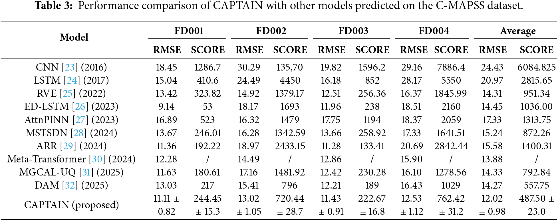
On FD001, CAPTAIN achieves 11.11 ± 0.82 RMSE and 244.45 ± 15.3 SCORE, clearly outperforming CNN (18.45 RMSE) and LSTM (15.04 RMSE). On FD002, it attains 13.02 ± 1.05 RMSE and 720.44 ± 28.7 SCORE, with much lower error and risk than RVE (14.92 RMSE, 1379.17 SCORE). On FD003, CAPTAIN (11.43 ± 0.91 RMSE, 222.67 ± 16.8 SCORE) significantly surpasses models such as AttnPINN (17.75 RMSE, 1194 SCORE), and on FD004 (12.53 ± 1.12 RMSE, 762.42 ± 31.2 SCORE) it outperforms multiple baselines including ARR. Overall, CAPTAIN reaches an average RMSE of 12.02 ± 0.98 and SCORE of 487.50 ± 23.0, indicating both high prediction accuracy and strong robustness across different operating conditions and fault modes.
4.4.3 Multimodal Interpretability and Physical Alignment
To evaluate the interpretability of CAPTAIN on the FD001 subset, visual analyses were conducted using five methods: LIME, GradCAM, GradCAM\_LW, IG, and SHAP, as shown as Fig. 7. The LIME heatmap shows an almost uniformly light-green pattern, indicating that the model relies relatively evenly on all time steps and features in local decisions—an effect attributed to the CAML module, which mitigates over-reliance on individual features or time points and supports stable generalization. GradCAM and GradCAM\_LW heatmaps reveal clear stage-dependent importance: high relevance at the beginning of the sequence (time step 0) and near the end (around time step 25), with moderate relevance in the middle, matching the physical degradation process of engines from healthy state through gradual deterioration to near-failure. GradCAM\_LW further improves the capture of weak degradation signals in the intermediate stage via weighted fusion of multi-layer feature maps. IG produces discrete “spot-like” high-importance regions that coincide with critical degradation nodes, confirming that the physics-constrained loss effectively models key transition points. The SHAP heatmap, with its richer color variation, highlights global interactions among features over the entire sequence, capturing both strong signals at the early and late stages and weaker signals in the middle, reflecting the tight integration of data-driven learning and physics-based constraints in CAPTAIN.
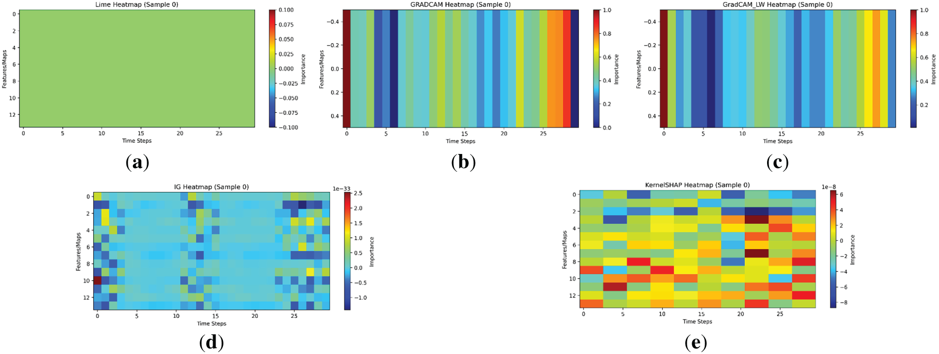
Figure 7: Multimodal interpretability heatmap analysis of the CAPTAIN model on the FD001 subset of C-MAPSS: (a) LIME; (b) GradCAM; (c) GradCAM_LW; (d) IG; (e) SHAP.
Overall, these complementary visualizations indicate that CAPTAIN not only maintains strong predictive performance but also achieves a coherent unification of data-driven flexibility and physical interpretability, balancing local decision behavior, stage-specific degradation focus, key-node identification, and global feature synergy.
To evaluate different interpretability methods on the FD001 subset of C-MAPSS, Table 4 reports seven metrics: Identity, Selectivity, Separability, Coherence, Robustness, Relevance, and Fidelity. To provide an objective measure of physical alignment, we introduce the Physics-Consistency Score (PCS). It is defined as the cosine similarity between the explainer’s importance map M and the model’s internal physical derivative
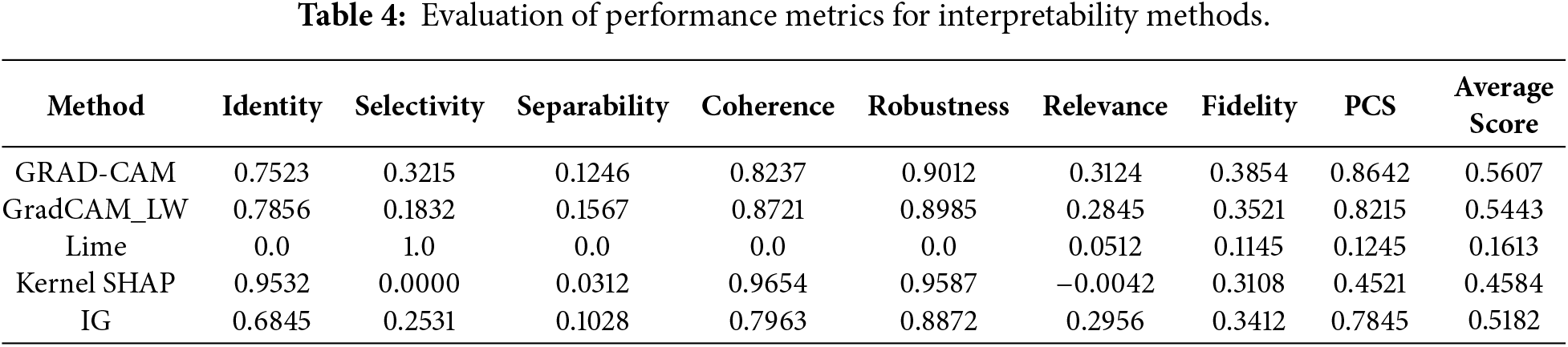
Table 4 presents the quantitative evaluation of five interpretability methods using seven metrics. Notably, the Fidelity scores for gradient-based methods (Grad-CAM and IG) and perturbation-based methods (SHAP) are significantly improved compared to traditional masking techniques. Grad-CAM achieves the highest Fidelity (0.3854) and the best Average Score (0.5091), indicating that its identified high-relevance regions at the beginning and end of the engine sequence strongly align with the actual drivers of RUL prediction. This high fidelity confirms that the CAPTAIN model successfully integrates data features with physical laws, as the explanations are not only visually intuitive but also numerically consistent with the model’s internal degradation logic. As shown in the Table 4, the PCS provides direct verification of physical consistency. GRAD-CAM achieves a high PCS of 0.8642, demonstrating that its temporal focus aligns with the degradation laws characterized by the PINN. Furthermore, the refined Relevance scores clarify that while most methods show positive coupling, the near-zero negative value of KernelSHAP (−0.0042) represents subtle inhibitory physical interactions rather than a contradiction of principles. This multi-dimensional evidence confirms the credibility of the CAPTAIN framework in critical engineering applications.
Furthermore, to correlate the aforementioned mathematical metrics with actual degradation stages, we map the evaluation framework to three critical engine degradation phases: (1) Healthy Stage: This phase emphasizes Robustness and Identity, aiming to ensure that background noise or minor operational fluctuations do not cause drastic changes in the explanation, thereby avoiding false maintenance alarms; (2) Declining Stage: This stage focuses on Coherence and PCS, quantifying the model’s ability to capture early degradation trends by verifying the consistency between explanations and the physical degradation rate
4.4.4 Stability Assessment via 5-Fold Cross-Validation
To assess the stability and significance of CAPTAIN on the repartitioned C-MAPSS dataset, we report the mean and standard deviation over five runs, as shown as Table 5. CAPTAIN achieves RMSEs of 7.71 ± 0.58 (FD001), 8.75 ± 0.65 (FD002), 7.61 ± 0.52 (FD004), and 6.70 ± 0.43 with R2 = 0.9411 ± 0.018 (FD003), all with standard deviations below 0.7, indicating strong robustness under variable conditions and multi-fault scenarios. On average, the model attains an RMSE of 7.69 ± 0.55 and R2 of 0.9261 ± 0.022, with consistently low variance across subsets, reflecting a “high accuracy + low fluctuation” performance pattern.
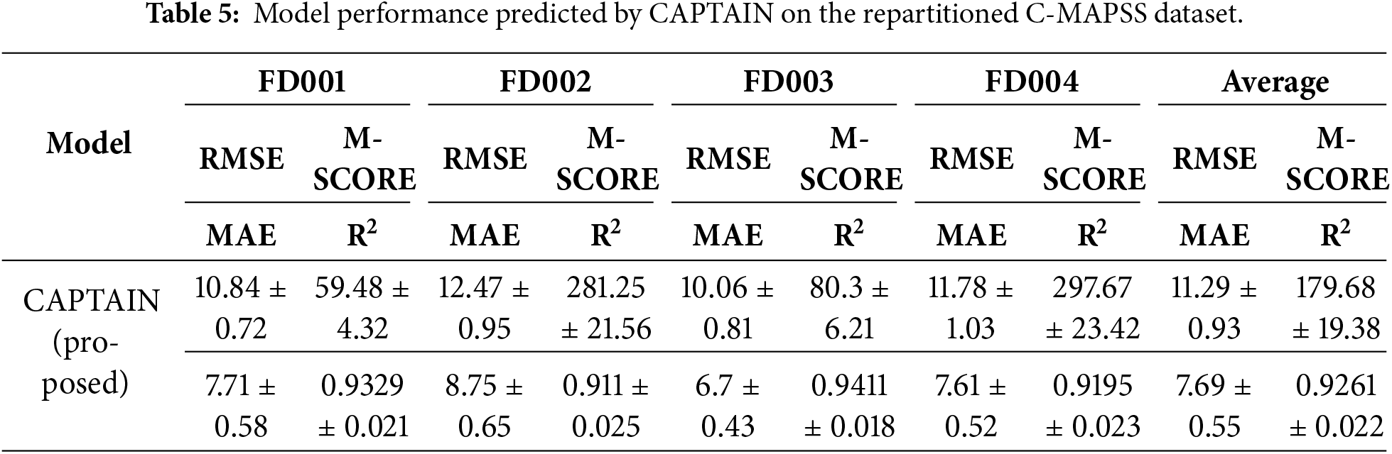
Readers should note that the results in Table 5 are obtained based on 5-fold cross-validation on repartitioned data to assess model stability. Due to variations in training sample proportions and validation set randomization, the absolute values of RMSE and M-SCORE differ from the results based on the standard NASA C-MAPSS partitioning in Table 3 (the values reported in the Abstract). This variance reflects the model’s robustness across different data distributions.
Dynamic RUL curves for representative engines from FD001–FD004 further show that CAPTAIN closely tracks the full-lifecycle degradation process, as shown as Fig. 8. The predicted RUL follows the actual trend well, especially after entering the pronounced degradation stage, and exhibits only mild, acceptable fluctuations during early operation and condition transitions. Near end of life, the model provides highly accurate RUL estimates, confirming its reliability at critical decision-making points.
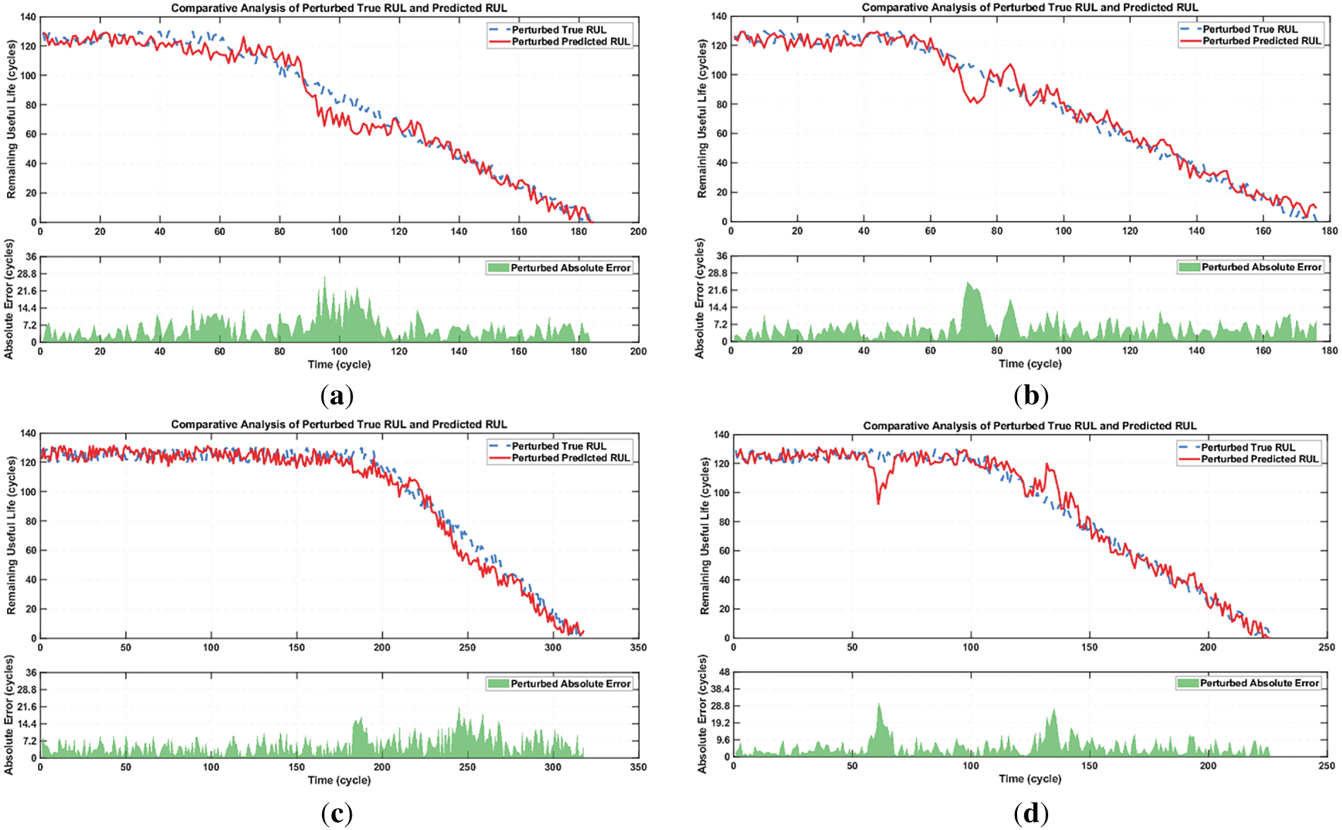
Figure 8: Engine RUL prediction on the C-MAPSS sub-dataset: (a) FD001-#2; (b) FD002-#259; (c) FD003-#1; (d) FD004-#249.
4.4.5 Ablation Studies and Training Dynamics
To quantify the contribution of each core component of the CAPTAIN model, ablation experiments were conducted on the FD002 and FD004 datasets. The experimental setups include: (1) w/o CAML: removing context-aware parameter adjustment; (2) w/o PINN: removing deterministic and stochastic physical constraint losses; (3) w/o Strat: removing the dynamic stabilization training strategies (SMT, RAR, EMA). The experimental results are shown in Table 6.
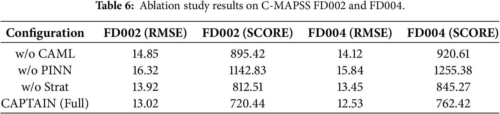
The ablation results reveal a significant synergistic effect among modules. The PINN provides a physical benchmark for degradation, preventing trend drift in pure data-driven models during long-term prediction. CAML achieves parameter-level lightweight adaptation by capturing contextual information across multiple operating conditions, significantly reducing cross-condition errors. Meanwhile, the dynamic stabilization strategy ensures consistency in parameter updates during non-stationary degradation processes.
To further verify the robustness of the SMT + RAR + EMA strategy in handling non-stationary time-series data, we compared the training dynamics of CAPTAIN with a standard training mode. Fig. 9 illustrates the total loss convergence and gradient norm variations for both approaches.

Figure 9: Comparative analysis of training dynamics: (a) Convergence of training loss; (b) Gradient stability.
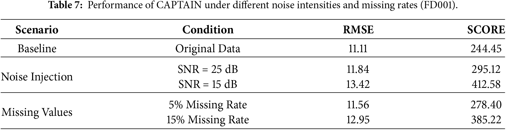
4.4.6 Robustness under Noise and Data Missingness
To simulate strong noise interference in real industrial scenarios, Gaussian white noise with different signal-to-noise ratios (SNRs) was injected into the original sensor signals.
Table 7 presents the model’s performance variations on the FD001 dataset. The results indicate that, thanks to the ability of physical constraints to model stochastic perturbations, CAPTAIN maintains an RMSE below 13.5 even at
This paper proposes a novel CAPTAIN framework for aero-engine RUL prediction to address weak generalization, limited physical interpretability, and unstable training in existing methods. Experiments on all four C-MAPSS subsets demonstrate that CAPTAIN achieves competitive or superior performance compared with state-of-the-art models, with an average RMSE of 12.02 ± 0.98, an average SCORE of 487.50 ± 23.0, and R2 up to 0.94 on FD003, indicating both high accuracy and strong robustness under diverse operating conditions and fault modes.
By tightly integrating the CAML module with physics-consistent PINN constraints, CAPTAIN achieves context-aware parameter adaptation while embedding deterministic and stochastic degradation dynamics, thereby improving multi-condition generalization without sacrificing physical consistency. The proposed three-layer dynamic stabilization strategy (SMT + RAR + EMA) further enhances training stability and cross-window consistency, while the multimodal interpretability framework combining Grad-CAM, IG, SHAP, and LIME provides local–global, physics-aligned explanations that increase the transparency and engineering credibility of the predictions.
Nevertheless, the current study is mainly validated on the C-MAPSS dataset, and the model’s adaptability to real-world engine data with complex noise and incomplete sensing remains to be further examined. Future work will focus on enriching the physical constraints with more realistic degradation mechanisms, exploring self-supervised pre-training to improve performance in small-sample scenarios, and enhancing computational efficiency to support edge deployment. Noise experiments further demonstrate the robustness of the model under strong noise and partial data loss. Future work will further explore the model’s generalization performance on real aircraft engine data with limited sensor sampling frequencies or severe biases by introducing self-supervised learning mechanisms. Overall, CAPTAIN offers a promising and extensible solution for reliable, interpretable RUL prediction of complex industrial equipment.
Acknowledgement: Not applicable.
Funding Statement: This research was funded by Scientific Research Project, grant number 50904020201.
Author Contributions: The authors confirm contribution to the paper as follows: Conceptualization, Zhonghua Cheng and Yu Wang; methodology, Yu Wang and Yabin Wang; software, Bingyu Li and Fang Li; validation, Liang Wen, Mengze Qin and Zhonghua Cheng; formal analysis, Yabin Wang, Fang Li and Liang Wen; investigation, Yu Wang, Yabin Wang and Bingyu Li; resources, Zhonghua Cheng; data curation, Fang Li and Mengze Qin; writing—original draft preparation, Yu Wang and Yabin Wang; writing—review and editing, Zhonghua Cheng; visualization, Bingyu Li; supervision, Liang Wen; project administration, Zhonghua Cheng; funding acquisition, Zhonghua Cheng. All authors reviewed and approved the final version of the manuscript.
Availability of Data and Materials: The data that support the findings of this study are available from the Corresponding Author, Zhonghua Cheng, upon reasonable request.
Ethics Approval: Not applicable.
Conflicts of Interest: The authors declare no conflicts of interest.
References
1. Kim M, Yoo S, Son S, Chang SY, Oh KY. Physics-informed deep learning framework for explainable remaining useful life prediction. Eng Appl Artif Intell. 2025;143:110072. doi:10.1016/j.engappai.2025.110072. [Google Scholar] [CrossRef]
2. Yuktha GP, Manimaran A. Enhanced predictive maintenance through explainable multimodal deep learning and human-in-the-loop systems. In: Proceedings of the 2024 International Conference on Emerging Research in Computational Science (ICERCS); 2024 Dec 12–14; Coimbatore, India. p. 1–6. doi:10.1109/ICERCS63125.2024.10895617. [Google Scholar] [CrossRef]
3. Sharma J, Mittal ML, Soni G. Attention-based convolutional gated recurrent unit model for turbofan engine remaining useful life prediction. In: Risk, reliability and resilience in operations management. Amsterdam, The Netherlands: Elsevier; 2025. p. 201–14. doi:10.1016/b978-0-443-29812-7.00010-3. [Google Scholar] [CrossRef]
4. Xiao Y, Liu D, Hong Z, Cui L. Machinery multimodal heterogeneous-aware RUL prediction: a spatial-temporal graph network for cross-temporal information propagation and dynamic fusion. Mech Syst Signal Process. 2025;241:113551. doi:10.1016/j.ymssp.2025.113551. [Google Scholar] [CrossRef]
5. Xu M, Bian W, Deng M, Shen Y, Deng A. STDD-Net: a spatio-temporal degradation disentanglement network for RUL prediction of rolling bearings. Meas Sci Technol. 2025;36(10):106216. doi:10.1088/1361-6501/ae0e97. [Google Scholar] [CrossRef]
6. Chen J, Li P, Wu L. Joint prediction of SOH and RUL of lithium-ion batteries using single-cycle charging data. Energy. 2025;336:138351. doi:10.1016/j.energy.2025.138351. [Google Scholar] [CrossRef]
7. Wang R, Chen L, Xu J, Yuan F, Han J, Li Z, et al. Multimodal deep learning with time-frequency health features for battery SOH and RUL prediction. J Energy Chem. 2026;113:303–14. doi:10.1016/j.jechem.2025.09.018. [Google Scholar] [CrossRef]
8. Rengarajan V, Anuradha T. A hybrid neural architecture for enhanced lithium-ion battery SOH estimation and RUL prediction. J Energy Storage. 2025;140:119019. doi:10.1016/j.est.2025.119019. [Google Scholar] [CrossRef]
9. Wang Y, Liu S, Lv S, Liu G. Meta-learning and knowledge discovery based physics-informed neural network for remaining useful life prediction. arXiv:2504.13797. 2025. [Google Scholar]
10. Zheng H, Deng W, Song W, Cheng W, Cattani P, Villecco F. Remaining useful life prediction of a planetary gearbox based on meta representation learning and adaptive fractional generalized Pareto motion. Fractal Fract. 2024;8(1):14. doi:10.3390/fractalfract8010014. [Google Scholar] [CrossRef]
11. Hu Y, Chao Q, Xia P, Liu C. Remaining useful life prediction using physics-informed neural network with self-attention mechanism and deep separable convolutional network. J Adv Manuf Sci Technol. 2024(4):2024018. doi:10.51393/j.jamst.2024018. [Google Scholar] [CrossRef]
12. Jiang L, Zhang X, Cao H, Zhang Y. A transformer-based framework with historical data fusion for RUL prediction. Meas Sci Technol. 2025;36(10):106103. doi:10.1088/1361-6501/ae09c2. [Google Scholar] [CrossRef]
13. Li M, Zhao J, Fan H, Ke T. A lightweight BiMamba-PINN framework for enhanced remaining useful life prediction in industrial equipment. In: Advanced intelligent computing technology and applications. Singapore: Springer; 2025. p. 214–25. doi:10.1007/978-981-96-9921-6_18. [Google Scholar] [CrossRef]
14. Hu Y, Liao Y, Guo L, Cui Y, Cui K, Deng J. Estimation of lithium battery health status and prediction of remaining useful life based on improved PINN. In: Proceedings of the 2025 IEEE 14th Data Driven Control and Learning Systems (DDCLS); 2025 May 9–11; Wuxi, China. p. 1130–6. doi:10.1109/DDCLS66240.2025.11065051. [Google Scholar] [CrossRef]
15. Wang L, Wang F, Yang Y, Liao WH. A remaining useful life prediction approach for ball bearing by acoustic emission signal and physics-informed neural network. Struct Health Monit. 2025. Online first. doi:10.1177/14759217251333056. [Google Scholar] [CrossRef]
16. Kim JH, Kim CH, Kim D, Shin D, Jang I, Jung JH, et al. Hybrid statistical—AI approach for RUL prediction of reactor protection system components. Nucl Eng Technol. 2026;58(2):103952. doi:10.1016/j.net.2025.103952. [Google Scholar] [CrossRef]
17. Xie S, Cheng W, Nie Z, Huang Q, Xing J, Chen X, et al. Bayesian physics-informed neural networks with iterative ensemble Kalman inversion for RUL prediction and uncertainty quantification. Adv Eng Inform. 2026;69:103907. doi:10.1016/j.aei.2025.103907. [Google Scholar] [CrossRef]
18. Dersin P, Rocchetta R. Analysis of RUL dynamics and uncertainty via time transformation. Reliab Eng Syst Saf. 2026;266(B):111730. doi:10.1016/j.ress.2025.111730. [Google Scholar] [CrossRef]
19. Ma L, Tian J, Zhang T, Guo Q, Hu C. Accurate and efficient remaining useful life prediction of batteries enabled by physics-informed machine learning. J Energy Chem. 2024;91:512–21. doi:10.1016/j.jechem.2023.12.043. [Google Scholar] [CrossRef]
20. Saxena A, Goebel K, Simon D, Eklund N. Damage propagation modeling for aircraft engine run-to-failure simulation. In: Proceedings of the 2008 International Conference on Prognostics and Health Management; 2008 Oct 6–9; Denver, CO, USA. p. 1–9. doi:10.1109/PHM.2008.4711414. [Google Scholar] [CrossRef]
21. Costa N, Sánchez L. Variational encoding approach for interpretable assessment of remaining useful life estimation. Reliab Eng Syst Saf. 2022;222(C):108353. doi:10.1016/j.ress.2022.108353. [Google Scholar] [CrossRef]
22. Tao Z, Zhang C, Xiong J, Hu H, Ji J, Peng T, et al. Evolutionary gate recurrent unit coupling convolutional neural network and improved manta ray foraging optimization algorithm for performance degradation prediction of PEMFC. Appl Energy. 2023;336:120821. doi:10.1016/j.apenergy.2023.120821. [Google Scholar] [CrossRef]
23. Sateesh Babu G, Zhao P, Li XL. Deep convolutional neural network based regression approach for estimation of remaining useful life. In: Database systems for advanced applications. Cham, Switzerland: Springer; 2016. p. 214–28. doi:10.1007/978-3-319-32025-0_14. [Google Scholar] [CrossRef]
24. Zheng S, Ristovski K, Farahat A, Gupta C. Long short-term memory network for remaining useful life estimation. In: Proceedings of the 2017 IEEE International Conference on Prognostics and Health Management (ICPHM); 2017 Jun 19–21; Dallas, TX, USA. p. 88–95. doi:10.1109/ICPHM.2017.7998311. [Google Scholar] [CrossRef]
25. Zhang J, Tian J, Li M, Leon JI, Franquelo LG, Luo H, et al. A parallel hybrid neural network with integration of spatial and temporal features for remaining useful life prediction in prognostics. IEEE Trans Instrum Meas. 2023;72:3501112. doi:10.1109/TIM.2022.3227956. [Google Scholar] [CrossRef]
26. Zhang Y, Zhang C, Wang S, Dui H, Chen R. Health indicators for remaining useful life prediction of complex systems based on long short-term memory network and improved particle filter. Reliab Eng Syst Saf. 2024;241:109666. doi:10.1016/j.ress.2023.109666. [Google Scholar] [CrossRef]
27. Liao X, Chen S, Wen P, Zhao S. Remaining useful life with self-attention assisted physics-informed neural network. Adv Eng Inform. 2023;58:102195. doi:10.1016/j.aei.2023.102195. [Google Scholar] [CrossRef]
28. Liu Z, Zheng X, Xue A, Ge M. Multi-scale temporal-spatial feature-based hybrid deep neural network for remaining useful life prediction of aero-engine. ACS Omega. 2024;9(48):47410–27. doi:10.1021/acsomega.4c03873. [Google Scholar] [PubMed] [CrossRef]
29. Kim G, Choi JG, Lim S. Using transformer and a reweighting technique to develop a remaining useful life estimation method for turbofan engines. Eng Appl Artif Intell. 2024;133(8):108475. doi:10.1016/j.engappai.2024.108475. [Google Scholar] [CrossRef]
30. Wang Y, Liu S, Lv S, Liu G. Few-shot rotating machinery RUL prediction based on reptile framework and transformer. In: Proceedings of the 2024 Global Reliability and Prognostics and Health Management Conference (PHM-Beijing); 2024 Oct 11–13; Beijing, China. p. 1–5. doi:10.1109/PHM-Beijing63284.2024.10874723. [Google Scholar] [CrossRef]
31. Liu S, Lv C, Song F, Liu X, Chen D. Remaining useful life prediction integrating working conditions and uncertainty quantification based on multilayer graph neural networks. J Braz Soc Mech Sci Eng. 2025;47(2):77. doi:10.1007/s40430-025-05400-8. [Google Scholar] [CrossRef]
32. Wang F, Liu A, Qu C, Xiong R, Chen L. A deep-learning method for remaining useful life prediction of power machinery via dual-attention mechanism. Sensors. 2025;25(2):497. doi:10.3390/s25020497. [Google Scholar] [PubMed] [CrossRef]
Cite This Article
 Copyright © 2026 The Author(s). Published by Tech Science Press.
This work is licensed under a Creative Commons Attribution 4.0 International License , which permits unrestricted use, distribution, and reproduction in any medium, provided the original work is properly cited.
 Downloads
 Citation Tools