AgroGeoDB-Net: A DBSCAN-Guided Augmentation and Geometric-Similarity Regularised Framework for GNSS Field–Road Classification in Precision Agriculture

1  Introduction

Field-road classification is a key task in smart agriculture, which distinguishes Global Navigation Satellite System (GNSS) trajectory points during in-field operations (field points) from those during road travel (road points). Accurate classification reduces manual interpretation and enhances field monitoring, route planning, and cultivated-area estimation [1,2]. However, GNSS trajectory data present three major challenges: (i) strong class imbalance, since agricultural machinery operates much longer within fields than on roads (Fig. 1); (ii) diverse operational heterogeneity across different machinery types and field conditions; and (iii) complex spatiotemporal dependencies that couple nonlinear motion behaviors with fine-grained spatial patterns. These characteristics make reliable classification particularly difficult.

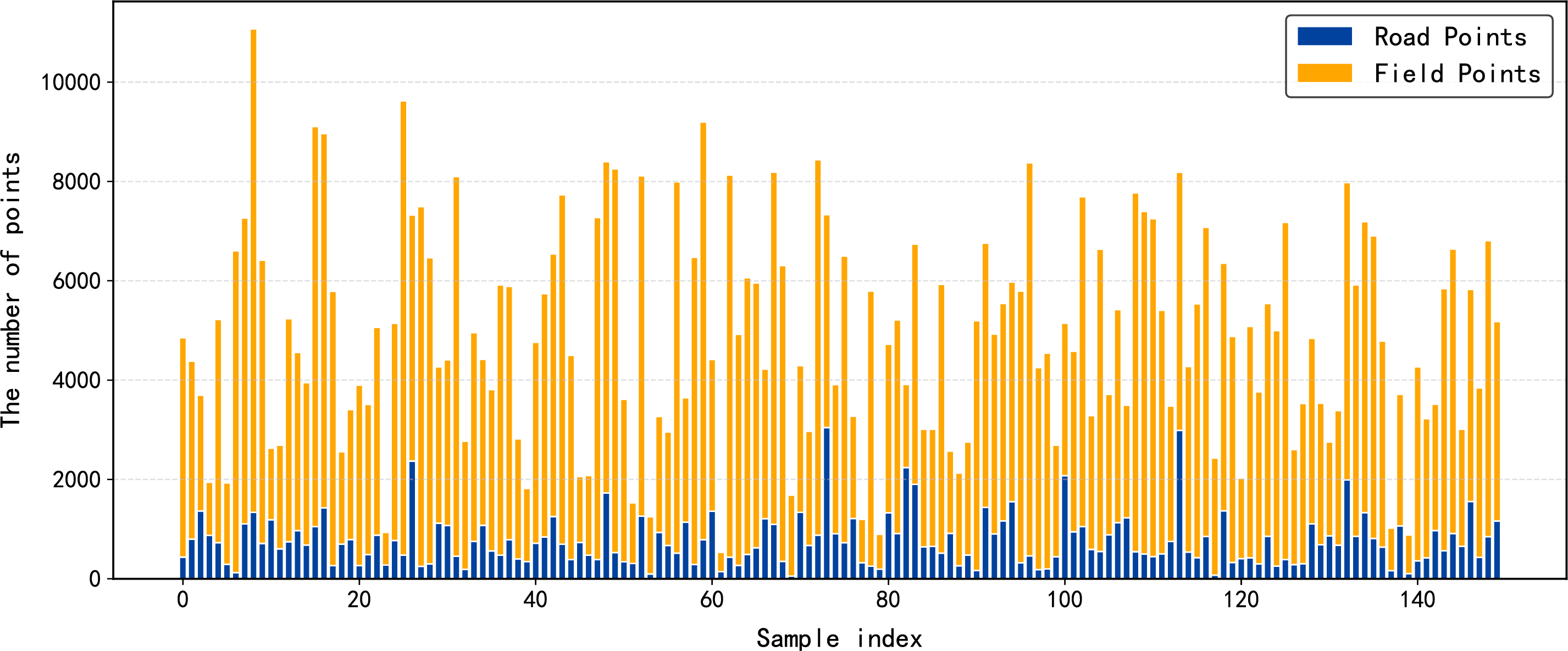
Figure 1: Illustration of class imbalance in GNSS trajectory data.

Trajectory classification has been extensively studied in the broader field of spatial trajectory data mining, with early work focusing on understanding human mobility patterns and extracting semantic movement information from GPS data through statistical analysis and pattern mining [3–5]. Building on these foundations, trajectory classification has been further explored in domains such as maritime surveillance, urban mobility [6], and traffic behaviour analysis [7]. In the transportation and public-safety literature, a substantial body of work has focused on learning discriminative trajectory representations to characterise movement patterns and distinguish between different agents or behaviours. Representative studies include trajectory embedding methods for human mobility identification [8], trajectory–user linking via generative or attention-based models [9,10], and hierarchical spatio-temporal architectures that jointly exploit local motion and long-range temporal context. These approaches demonstrate that deep representation learning can effectively capture semantic information from raw or weakly processed trajectories, often outperforming traditional handcrafted feature pipelines.

Despite these advances, agricultural trajectory classification presents a distinctly different problem setting. Field–road discrimination in agricultural operations is characterised by extreme class imbalance, sparse and irregular sampling, strong spatial heterogeneity, and operation-specific motion patterns that differ fundamentally from urban or transportation scenarios. In particular, agricultural GNSS trajectories are typically low-information-density signals [11], where semantic cues must be inferred from subtle geometric and density characteristics rather than from rich contextual information. These differences necessitate dedicated modelling strategies that go beyond directly transferring existing traffic-trajectory classification methods.

Existing studies on field–road classification can be broadly divided into two methodological categories: traditional machine learning and deep learning approaches. Traditional methods commonly rely on handcrafted descriptors and classical classifiers. For example, Chen et al. [12] combined a clustering strategy (DBSCAN [13]) with rule-based inference, while Poteko et al. [14] employed decision-tree classifiers based on motion statistics. These methods provide interpretable decision processes and are computationally lightweight, but their effectiveness depends strongly on expert-designed features and parameter calibration. Consequently, they often fail to capture the nonlinear spatial–temporal dependencies and behavioral variability inherent in agricultural trajectory data. With the growing availability of GNSS observations, deep learning models have been increasingly applied to this task. Bian et al. [15] integrated convolutional layers, Transformer encoders, and bidirectional LSTM networks to enhance sequential modelling. Related studies have further explored BiLSTM-based designs for agricultural trajectory analysis, including velocity-enhanced and graph-aware variants, to better capture motion dynamics and temporal continuity [16–18], while Chen et al. [19] transformed trajectories into spatial–temporal images and applied an Attention U-Net for feature extraction. Zhai et al. [20] proposed a dual-domain context-aware network for agricultural machinery trajectory operation mode identification, modelling trajectory data as multivariate time series and integrating enriched kinematic features with temporal and contextual representations. Although these models demonstrate superior performance compared with conventional approaches, they still face common limitations: inadequate treatment of severe class imbalance between field and road samples, limited incorporation of spatial distribution cues such as point density and directional consistency, and insufficient interpretability when applied to heterogeneous agricultural environments. These issues continue to motivate the development of more robust and geometry-aware frameworks for field–road classification.

Our earlier deep learning approach [21] introduced a density-guided method for field–road classification. However, that work processed trajectory points largely in isolation, under-utilising long-range temporal context, and its variational encoder lacked a unified mechanism to jointly capture spatial distribution cues and motion dynamics. Building on these insights, this article presents AgroGeoDB-Net, a framework that incorporates comprehensive spatio-temporal representation learning and geometry-aware regularisation for robust field–road classification.

The main contributions of this work are summarized as follows:

1.   We design a Density-Aware Local Interpolator (DALI) and an accompanying spatial–motion descriptor module that, respectively, oversample minority road points via cluster-wise interpolation and encode each point’s local density, directional alignment, inter-point spacing, and kinematic derivatives, thus alleviating class imbalance while supplying geometry-rich inputs for downstream modelling.

2.   We present AgroGeoDB-Net, which integrates a geometry-aligned hybrid motion–spatial encoder trained with a density-weighted focal loss and a density-regularised KL term to balance temporal modelling and spatial structure preservation.

3.   We validate AgroGeoDB-Net on five trajectory datasets, demonstrating superior classification accuracy and robustness to sparse sampling, GNSS noise, and operational heterogeneity when compared with both traditional classifiers and recent deep-learning baselines.

Beyond individual architectural components, the core novelty of this work lies in formulating a density-centric modeling framework for GNSS-based field–road discrimination, in which local point density is embedded as an explicit inductive bias across multiple stages of the network. Unlike prior approaches that use density as an isolated feature, heuristic rule, or post hoc reweighting factor, AgroGeoDB-Net integrates density coherently into representation learning and objective design. In particular, a KL-regularised latent encoder aligns feature distributions with local density structure, while a residual BiLSTM jointly exploits this geometry-aligned representation and long-range temporal context for robust sequence modelling. This coordinated interaction between density-aware latent encoding and residual temporal modelling distinguishes the proposed framework from ad hoc combinations of clustering, loss reweighting, and sequence models, and goes beyond an incremental integration of standard components, as summarised in Table 1.

2  Methods

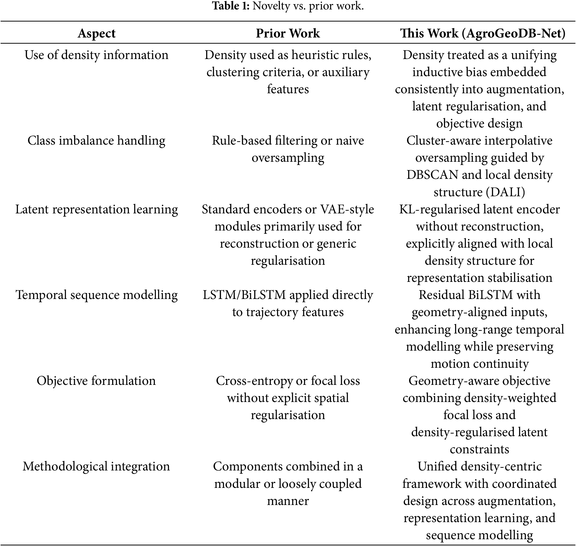
Fig. 2 summarises the overall workflow. Starting from raw GNSS trajectories, the Density-Aware Local Interpolator first removes duplicated or noisy points, smooths small-scale fluctuations, and performs DBSCAN-guided local interpolation to balance field–road samples, with detailed implementation described in Appendix A. The cleaned and augmented trajectories are then transformed into a Motion–Spatial Descriptor Module that combines kinematic attributes (speed, acceleration, angular velocity) with spatial descriptors (local density, parallel relation, inter-point distance), resulting in a 14-dimensional representation for every trajectory point. These feature sequences serve as the input for model training: the KL-regularised latent encoder produces geometry-aware latent embeddings, and the residual BiLSTM sequence modeller captures bidirectional temporal structure. A linear classifier is finally applied to the learned contextual representations, and the trained AgroGeoDB-Net is used to infer field–road labels for unseen trajectories.

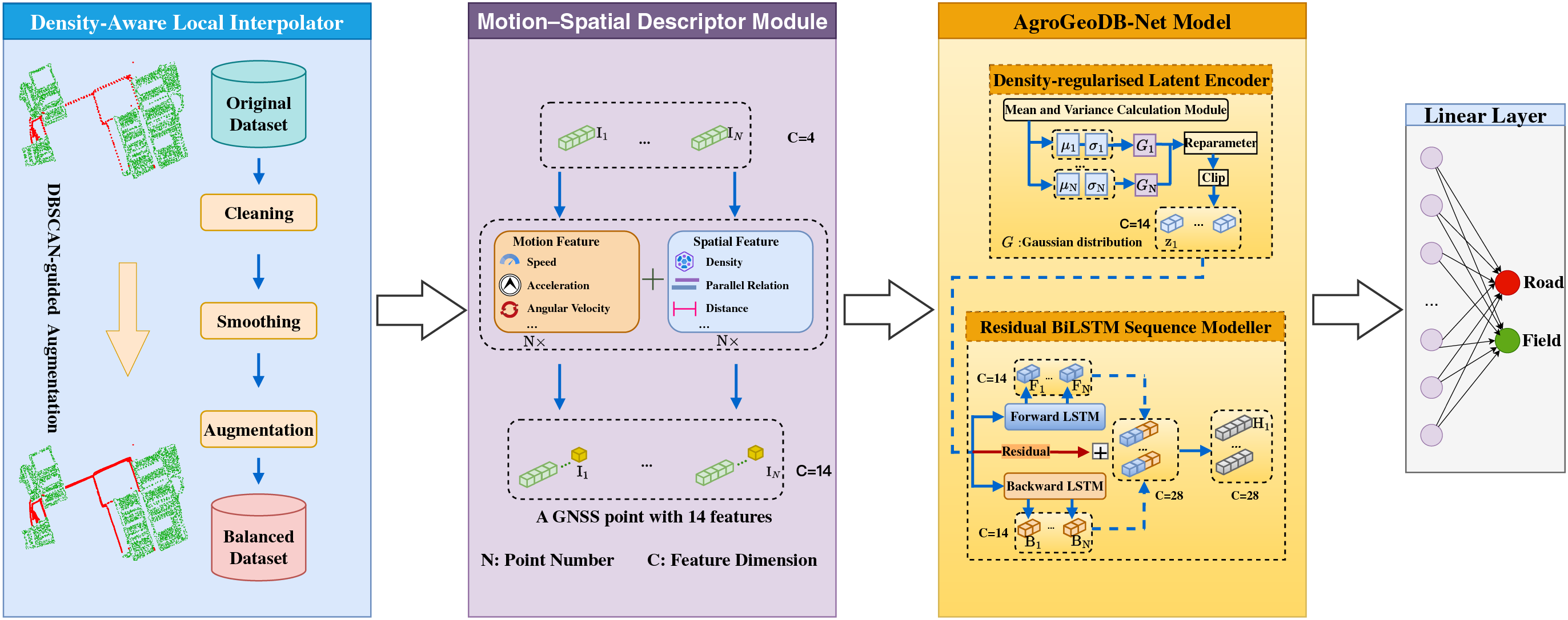
Figure 2: Overall framework of the proposed method.

2.1 Density-Aware Local Interpolator (DALI)

Let the raw trajectory be 𝒫={pi=[loni,lati,ti]}i=1n, where each point records longitude, latitude and timestamp. By deriving the instantaneous speed vi and heading angle θi from successive positions and times, we obtain the enriched sequence 𝒫~={p~i=[loni,lati,vi,θi]}i=2n, in which vi measures the travel speed between pi−1 and pi, and θi denotes the bearing of motion at pi. This four-dimensional representation serves as the input. DALI then proceeds in two sequential steps: (i) DBSCAN-based road clustering that groups geometrically contiguous road points, followed by (ii) cluster-wise linear interpolation that densifies each road fragment while preserving its spatial coherence.

2.1.1 DBSCAN-Based Road Clustering

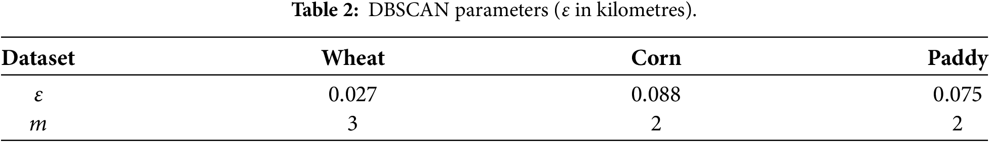
DBSCAN partitions 𝒫~ into coherent road fragments according to two parameters: neighbourhood radius ε and minimum samples m

Nε(p)={q∈𝒫~∣‖q−p‖≤ε},p core ⟺ |Nε(p)|≥m.(1)

Neighbourhood radius ε. A proper ε must be large enough to bridge successive points on the same road but smaller than the gap that separates different roads. Formally,

dmax<ε<dmin,(2)

where dmax is the largest inter-point spacing within a single road and dmin the smallest distance between two parallel or intersecting roads. As a general trend, smaller ε yields finer, more fragmented clusters, whereas larger ε produces coarser, more aggregated clusters, as illustrated in Fig. 3.

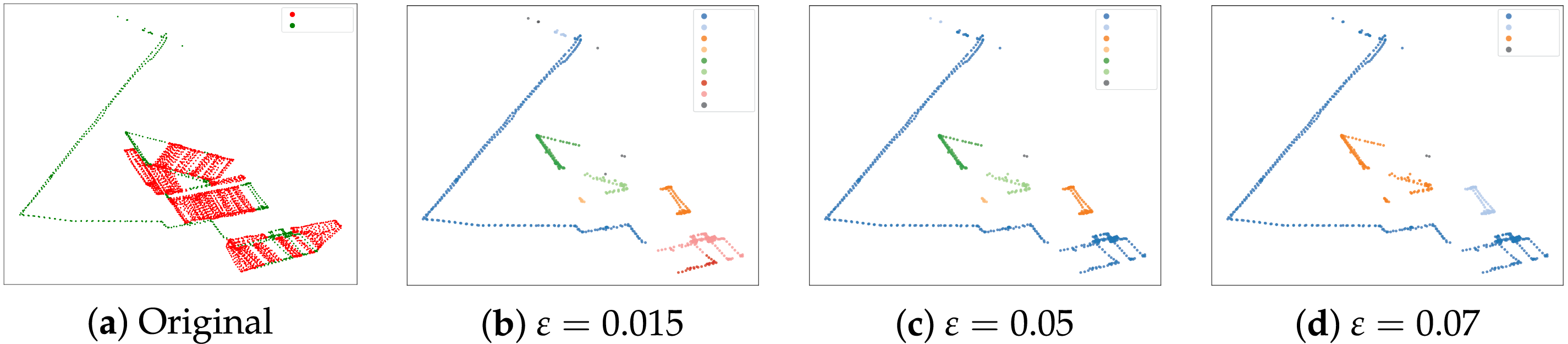
Figure 3: Effect of neighbourhood radius ε on clustering granularity.

Automatic selection. Step 1–3—distance curve. For each p~i, compute k-dist (p~i), the distance to its third-nearest neighbour (k=3). Sorting these values in descending order yields the 3-distance curve; its point of maximum curvature, denoted εknee, provides a data-driven estimate of dmax.

Step 2—stability search. Set ε=αεknee with a scale factor α∈[0.7,1.3]. This interval corresponds to a ±30% variation around the knee-point estimate, reflecting the empirically observed stability range of density-based clustering. It ensures that ε remains close enough to the intrinsic neighbourhood scale to avoid both over-segmentation (α<0.7) and over-merging (α>1.3). Such proportional adjustment has been widely adopted as a heuristic in automatic parameter tuning of DBSCAN and its variants [13,22,23]. Run DBSCAN; increase (decrease) α when a physical road is split (merged) until each real-world road forms one cluster. Because ε never exceeds the first inter-road gap encountered, the condition ε<dmin is satisfied implicitly.

Step 3—dataset-level fixing. The resulting ε values are fixed per dataset (Table 2).

Under these dataset-fixed settings, we further examine the statistical relationship between local neighbourhood density Nε(⋅) and operational labels (field vs. road) at dataset levels. The corresponding empirical analysis is reported in Appendix B.

Minimum samples m. To maintain a consistent notion of local density across datasets with different spatial resolutions, the minimum samples parameter m is determined adaptively from the nominal sampling rate of road points. Let froad∈[0.1,1] Hz denote the average GNSS sampling frequency along the road, and set a safety factor β=2 to tolerate occasional gaps or positioning jitters. Then

m=⌈βfroad⌉.(3)

This formulation ensures that each core point must have at least two to three neighbours within its ε-neighbourhood, i.e., m∈{2,3} (Table 2). In essence, m scales with the effective sampling density of the road, providing an adaptive density threshold that prevents over-fragmentation in sparsely sampled areas while avoiding excessive merging in dense regions.

2.1.2 Cluster-Wise Linear Interpolation

For every road fragment 𝒞={p~(1),…,p~(|𝒞|)} retrieved by DBSCAN, points are first ordered by their timestamps. Let

dj=‖p~(j+1)−p~(j)‖,Δθj=|θ(j+1)−θ(j)| (mod360∘),(4)

denote the inter-point distance and heading difference of successive samples. Interpolation between p~(j) and p~(j+1) is carried out only when both geometric consistency conditions defined by the clustering configuration are satisfied:

dj≤ε,Δθj≤Θmax=30∘.(5)

Distance constraint. The condition dj≤ε ensures that all interpolated points remain within the same ε-neighbourhood established during DBSCAN clustering. This constraint preserves the original local connectivity of the density graph and prevents interpolation across spatial gaps that violate the clustering structure.

Direction (course difference) constraint. The angular bound Θmax=30∘ limits the maximum allowable change in heading between consecutive trajectory points. It serves as a geometric consistency constraint that prevents physically implausible direction changes during interpolation, such as abrupt turns or spurious shortcuts across non-collinear road segments, while preserving local directional coherence along realistic vehicle motion.

Interpolation density and placement. Let vavg be the global mean nearest-neighbour spacing of road points. The number of interpolated points is

nj=⌊dj/vavg⌋,(6)

and their positions are distributed uniformly:

xj,k=p~(j)+knj+1(p~(j+1)−p~(j)),k=1,…,nj.(7)

Because nj scales with the actual gap dj, denser sampling is introduced only where the trajectory is genuinely sparse; conversely, closely spaced pairs remain unchanged.

2.2 Motion–Spatial Descriptor Module

Following the density-aware augmentation in Section 2.1, the enriched trajectory 𝒫~={p~i=[loni,lati,vi,θi]} provides a geometrically coherent and densified representation of each trajectory segment identified by DBSCAN. Based on this representation, the Motion–Spatial Descriptor Module maps each enriched trajectory point to a 14-dimensional feature vector fi∈R14, which serves as the input to the downstream geometry-aligned latent encoder.

The purpose of this module is not to perform feature selection, but to explicitly encode physically meaningful motion and spatial cues that are difficult to infer reliably from sparse GNSS observations alone. Given the limited raw signals available (longitude, latitude, timestamp, speed, and bearing), the constructed descriptors provide a structured and informative representation that complements subsequent representation learning. Potential correlations or partial redundancy among feature dimensions are therefore intentionally permitted, allowing the learning model to automatically exploit, reweight, or suppress correlated information during training.

Specifically, the 14-dimensional feature vector fi is organised into three complementary groups of descriptors:

•   Motion kinematics (9 dims)

      –   Speed profile: Δvi=vi−vi−1, ai=Δvi/Δti.

      –   Heading dynamics: Δθi=(θi−θi−1)mod360∘, angular velocity ωi=Δθi/Δti, angular acceleration αi=(ωi−ωi−1)/Δti.

      –   Displacements: Δlati, Δloni between successive samples.

      –   Path geometry: geodesic distance di and curvature ki=(θi−θi−1)/[(di+di−1)/2].

•   Local spatial distribution (3 dims)

      –   Point density Ni inside a 40 m × 20 m rectangle centred on p~i and aligned with θi.

      –   Directional coherence: mean θmeani and standard deviation θstdi of heading differences within the same rectangle.

•   Multi-scale spacing context (2 dims)

      –   Short-window spacing SD(i) over Lshort=5 points.

      –   Long-window spacing LD(i) over Llong=10 points.

These fourteen features jointly encode instantaneous movement, local geometry, and broader spacing trends, forming a compact representation for field–road classification.

2.3 AgroGeoDB-Net Model

Given the 14-dimensional motion–spatial descriptors ℱ={fi}i=2n constructed from the DALI-enhanced trajectory 𝒫~, AgroGeoDB-Net maps each point to field–road logits through three core components: (i) a density-regularised latent encoder that maps each descriptor fi to a latent embedding zi, forming the sequence {zi}; (ii) a residual bidirectional LSTM that captures bidirectional temporal dependencies and outputs contextual states {hi}; and (iii) a linear prediction head. The following subsections detail these components and the geometry-aware training objective that jointly governs them.

2.3.1 Density-Regularised Latent Encoder

As illustrated in Fig. 4, each handcrafted motion–spatial descriptor xi∈R14 is first fed into the Mean & Variance Calculation Module, which is implemented as a lightweight MLP that estimates the parameters of a Gaussian latent distribution. Concretely, it outputs the mean and the log-variance log⁡σi2 as

(μi,log⁡σi2)=MLP(xi),σi=exp⁡(0.5clip⁡(log⁡σi2,−2,2)).(8)

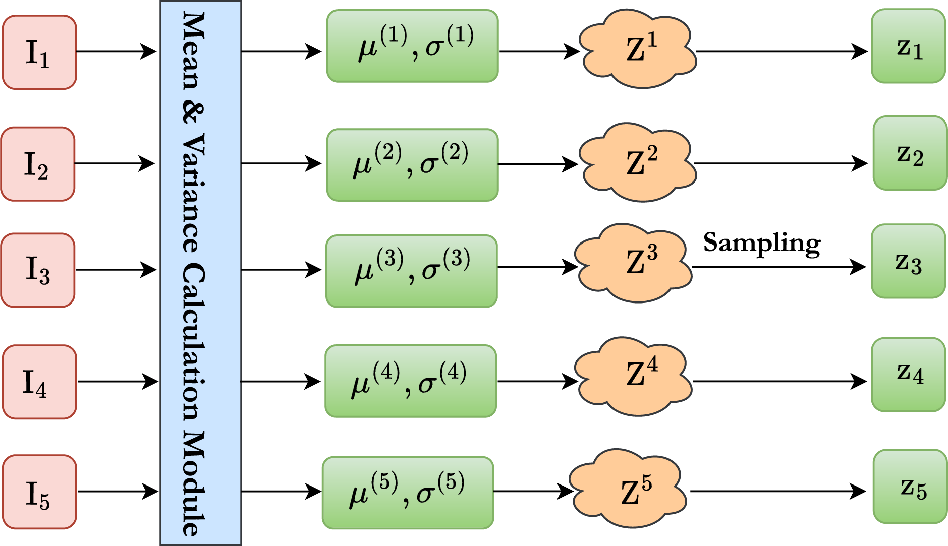
Figure 4: Density-regularised latent encoder.

Re-parameterisation sampling then produces the latent embedding

zi=μi+εiσi,εi∼𝒩(0,1).(9)

The divergence from the unit Gaussian prior is

KLi=12∑d=114(1+log⁡σi,d2−μi,d2−σi,d2),(10)

where the KL divergence is computed elementwise over the 14 latent dimensions.

Point-cloud density is used as a proxy for operation saliency: repeated in-field coverage produces dense point clouds, whereas road runs are much sparser. To inject this geometric context into the latent space, we introduce a density-regularised KL term, in which the divergence is weighted by the DBSCAN neighbourhood size introduced in Section 2.1,

wi=|Nε(pi)|,ℒKL=β∑iwiKLi,(11)

where Nε(pi) is the ε-neighbourhood of pi and β is a global factor. This adaptive weighting forces latent embeddings in high-density field regions to contract onto a compact, stable manifold, while allowing greater flexibility in low-density road segments. In this way, the KL regularisation is modulated by local trajectory density, aligning the learned latent space with the underlying geometry of agricultural behaviour.

2.3.2 Residual BiLSTM Sequence Modeller

The latent sequence {zi}i=1L is encoded by a two-layer bidirectional LSTM. At each layer, the forward and backward hidden states are concatenated and augmented with a residual shortcut from the input embedding zi, as illustrated in Fig. 5. Formally, the l-th layer output at position i is

hi(l)=BiLSTM(l)(hi(l−1))+Wreszi,l=1,2,(12)

with hi(0)=zi. Each BiLSTM has a hidden size of 14 per direction, so hi(l)∈R28. The final representation hi=hi(2) is fed into a linear head to produce the two output logits.

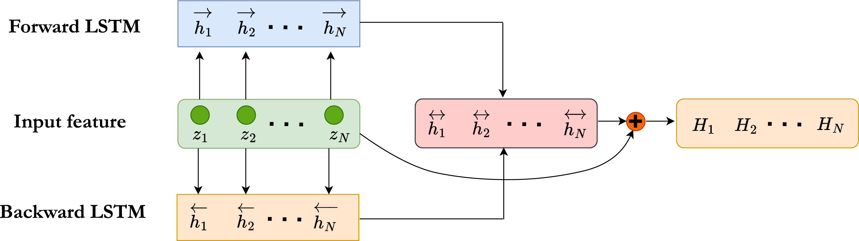
Figure 5: Residual bidirectional LSTM modeller.

The residual pathway in Fig. 5 ensures that the original per-point geometric cues in zi are directly preserved throughout the sequence modelling, while the bidirectional LSTMs accumulate long-range temporal context. This design stabilises optimisation and prevents the geometric signal from being overwritten by recurrent transformations.

2.3.3 Geometry-Aware Optimisation Objective

The network is trained end-to-end with a geometry-aware objective that combines a DBSCAN-weighted focal classification term with the density-regularised KL divergence introduced in Section 2.3.1. Together they couple point-wise classification fidelity with a trajectory-aware latent structure.

1) DBSCAN-weighted focal classification loss. Let yi∈{0,1} be the ground-truth label of point pi and ℓi∈R2 the corresponding logits. Denote pi=softmax⁡(ℓi)yi and reuse the neighbourhood weight wi=|Nε(pi)|. The imbalance-aware focal loss is

ℒfoc=1N∑i=1Nwiα(1−pi)γ(−log⁡pi),(13)

where α and γ follow the standard focal formulation. The DBSCAN-based weight wi further emphasises samples located in dense trajectory regions, reflecting their higher operational saliency.

2) Density-regularised KL divergence. As detailed in Section 2.3.1, the encoder associates each latent embedding zi with a KL term KLi measuring its divergence from the unit Gaussian prior. To inject trajectory geometry into the latent space, we modulate this divergence by the same DBSCAN neighbourhood size wi,

ℒKL=β∑iwiKLi,(14)

where β is a global scaling factor. This density-aware weighting forces latent embeddings in high-density field regions to contract onto a compact, stable manifold, while allowing greater flexibility in sparse road segments.

Total loss. The overall training objective is then

ℒ=ℒfoc+ℒKL.(15)

Since the logits ℓi are computed from the residual BiLSTM outputs hi, gradients from both terms jointly optimise the point-wise representation (latent encoder) and the temporal modelling layers (BiLSTM), producing latent trajectories that are both discriminative for field–road classification and consistent with the underlying spatial–temporal structure.

3  Experiments

AgroGeoDB-Net is assessed on five realworld GNSS trajectory datasets. The evaluation suite comprises (i) a baseline comparison against four published methods, (ii) an ablation that quantifies the individual gains of the residual BiLSTM sequence modeller and the density-aware local interpolator (DALI), and (iii) a cross-dataset generalisation test that trains on Wheat, Paddy and Corn and, following Section 3.6, is evaluated on the unseen Harvester and Tractor sets. All metrics are averaged over ten disjoint trajectory-level folds.

3.1 Experimental Settings

All experiments are conducted on an Intel Xeon (Ice Lake) CPU and a single NVIDIA A100 (40 GB) GPU under Ubuntu 22.04 LTS, CUDA 12.4, PyTorch 2.1, and Python 3.10. All reported results are obtained using 10-fold cross-validation at the trajectory level. In each fold, one fold is held out as the test set and is not used during training or validation. The remaining folds constitute the training pool of the current fold, within which trajectories are further split in a strictly trajectory-wise manner into training and validation subsets following an 80%/10% ratio for model optimisation and early stopping. Mini-batches of 32 trajectories are sampled with shuffling.

The network is optimised with AdamW (learning rate 5×10−4, weight decay 10−5) for at most 400 epochs. Validation is performed every ten epochs, and early stopping is triggered when the mixed metric

MIX=0.3Acc+0.3F1+0.2Pre+0.2Rec(16)

fails to improve for ten consecutive validations.

For each cross-validation fold, DBSCAN clustering, DALI-based interpolation, and all density-related statistics are computed exclusively using the training split of that fold; validation and test trajectories are never used to fit, tune, or influence any augmentation procedures or density statistics. During validation and testing, the model is evaluated exclusively on the original (raw) trajectory points, and no augmented points are introduced.

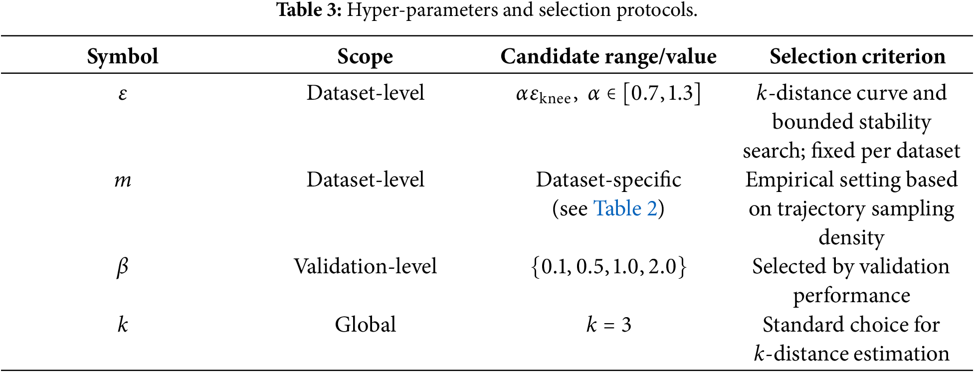
The proposed framework involves a small number of standard hyper-parameters operating at different scopes. All DBSCAN-related parameters, including the neighbourhood radius ε and minimum samples m, are determined once per dataset using the data-driven procedure described in Section 2.1 and are kept fixed throughout training and evaluation. The neighbourhood size wi=|Nε(pi)| is fully determined by ε and the local trajectory geometry, and is not treated as a tunable parameter.

The density-regularised latent encoder introduces a single global weighting parameter β that controls the strength of the KL regularisation term.

ℒKL=β∑iwiKLi.(17)

The parameter β is selected on the validation set via grid search over {0.1,0.5,1.0,2.0}, and the same value is used across all datasets. No hyper-parameters are tuned at the individual trajectory or point level.

Table 3 summarises all hyper-parameters, their scopes, and selection criteria.

3.2 Dataset

The core experiments use three in-domain GNSS collections gathered by China Agricultural University: Wheat (sampling 5 s), Paddy (30 s) and Corn (1 s). Every record stores timestamp, longitude, latitude, speed (m/s) and heading (deg, WGS-84) and is manually annotated as field or road.

Generalisation is tested on two additional sets acquired with the same protocol: Harvester (2 s, 100 trajectories, 1.15 M points, Shandong province) and Tractor (mixed sampling, 60 trajectories, 1.07 M points, six provinces).

3.3 Baseline Methods and Evaluation Metrics

Baseline Methods. We compare AgroGeoDB-Net against four representative field-road classification approaches that differ in both modelling strategy and feature design: DBSCAN+Rules [12], Decision Tree (DT) [14], Graph Convolutional Network (GCN) [24], and a pixel-level fusion model (STF+VFAU+BiLSTM) [19].

These baselines span a broad spectrum of input features. DBSCAN+Rules operates in an unsupervised manner directly on the five raw GNSS attributes recorded at each point. DT relies on handcrafted statistical descriptors, whereas GCN constructs an eight-dimensional relational feature set prior to message passing. STF+VFAU+BiLSTM incorporates additional visual cues by fusing statistical trajectory features with pixel-level remote-sensing representations. Among them, only DBSCAN+Rules is unsupervised; DT, GCN, STF+VFAU+BiLSTM, and our method are all supervised models.

Evaluation Metrics. Field–road classification is evaluated using multiple performance metrics to account for severe class imbalance. Unless otherwise stated, field is treated as the positive class to remain consistent with prior work. For imbalance-aware evaluation, the road class is additionally treated as the positive class.

We report Precision (Pre), Recall (Rec), F1-score (F1), and Accuracy (Acc), defined as

Pre=TPTP+FP,Rec=TPTP+FN,(18)

F1=2Pre⋅RecPre+Rec,Acc=TP+TNTP+TN+FP+FN.(19)

To further account for class imbalance, we additionally report Balanced Accuracy, Matthews Correlation Coefficient (MCC), and Precision–Recall AUC (PR-AUC), all computed with road treated as the positive class.

3.4 Overall Performance Comparison

We conducted comparative experiments on the Wheat, Paddy, and Corn datasets to evaluate the performance of AgroGeoDB-Net. All results are reported as mean ± standard deviation over 10-fold cross-validation to reflect both average performance and variability across folds. Table 4 summarises the classification performance of five field–road classification methods on these datasets. On the Wheat dataset, AgroGeoDB-Net achieved an Accuracy of 98.62±0.32% and an F1-score of 97.77±0.49%, outperforming the strongest baseline (STF+VFAU+BiLSTM) by a clear margin. The small standard deviations indicate highly stable performance across folds. For the Paddy dataset, AgroGeoDB-Net reached 93.35±1.14% Accuracy and 92.27±1.40% F1-score, exceeding the best baseline (GCN) by substantial margins while maintaining consistent fold-level behaviour. On the Corn dataset, AgroGeoDB-Net obtained an Accuracy of 95.46±1.27% and an F1-score of 92.58±2.23%. Although the relative improvements over STF+VFAU+BiLSTM are smaller than those observed on Wheat and Paddy, the results consistently favour AgroGeoDB-Net across all folds. The larger standard deviation on Corn reflects increased variability in operating conditions and sampling characteristics, which poses a more challenging classification scenario. Overall, AgroGeoDB-Net consistently outperforms all baseline methods across all three datasets under identical cross-validation protocols, demonstrating both strong average performance and reliable stability across folds.

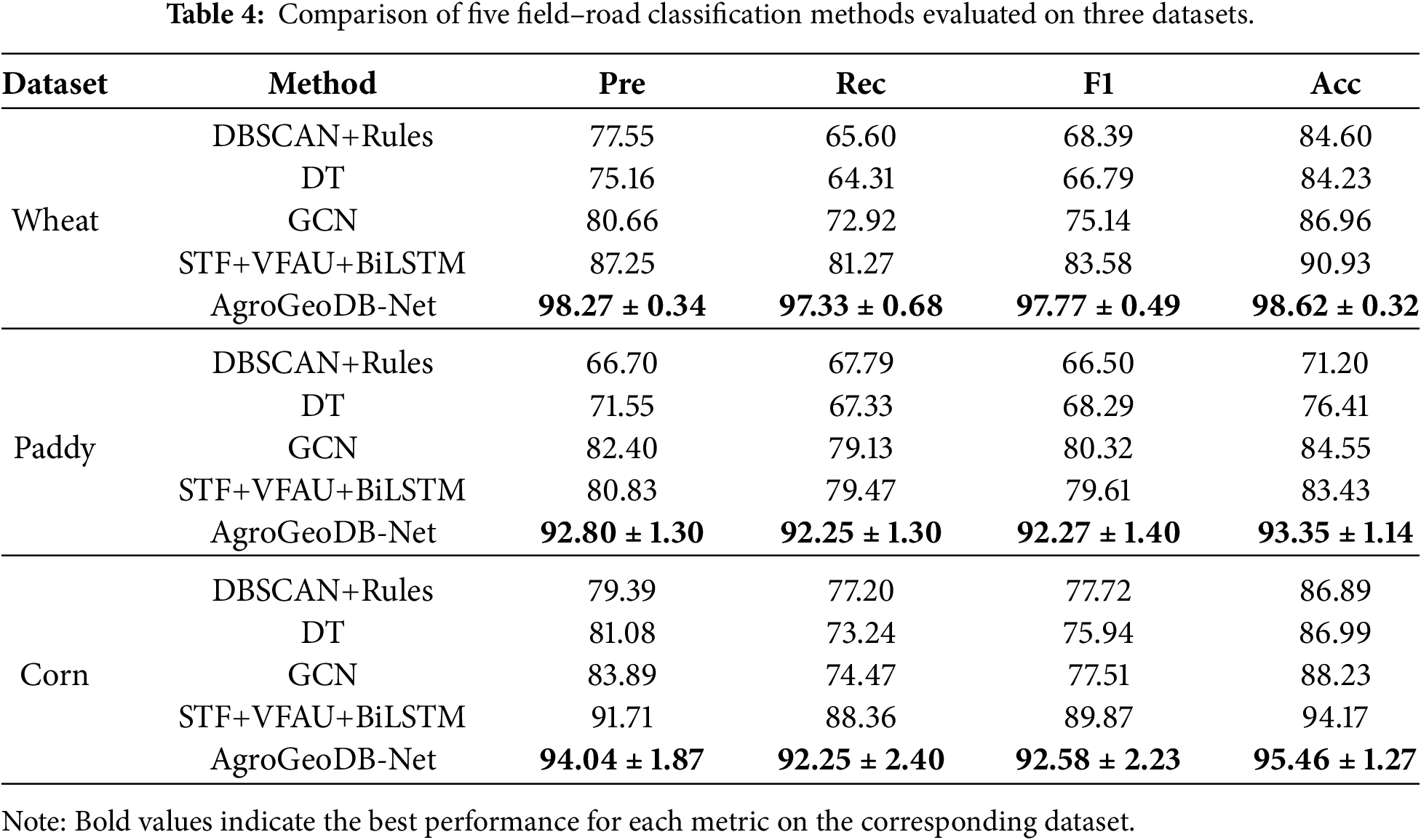
The performance differences among the five field-road classification methods can be attributed to their varying capabilities in extracting both motion and spatial distribution features from trajectory points. As noted by Chen et al. [24], DBSCAN+Rules is an unsupervised method that relies on spatial clustering relationships between trajectory points, leveraging density analysis to identify structural patterns in the trajectory. In contrast, the Decision Tree (DT) is a supervised learning method. Although it treats each trajectory point as an independent sample during modeling, its feature extraction process incorporates temporal relationships between points, partially compensating for its limited ability to model sequential dependencies. The GCN and STF+VFAU+BiLSTM methods further enhance spatiotemporal modeling capabilities by employing different types of neural network architectures to extract deep features from spatiotemporal adjacency among points. Specifically, GCN constructs a spatiotemporal graph structure of trajectory points and performs graph convolution operations to aggregate features within each point’s local neighborhood, effectively modeling spatiotemporal dependencies. STF+VFAU+BiLSTM, on the other hand, transforms trajectories into image representations and extracts visual features to encode spatial and temporal relationships from the trajectory images.

Compared with the above methods, AgroGeoDB-Net combines the strengths of statistical descriptors and deep representation learning in a unified architecture. It first derives informative motion and spatial-distribution features for each trajectory point through lightweight statistical rules. These descriptors are then refined by a density-regularised latent encoder, which learns geometry-aware latent embeddings, and further processed by a residual bidirectional LSTM that captures long-range temporal dependencies without losing local geometric cues. This multi-stage, hybrid feature extraction pipeline enables AgroGeoDB-Net to model spatiotemporal dynamics more comprehensively, resulting in markedly stronger discrimination of complex field–road trajectories.

3.5 Ablation Studies

To systematically validate the effectiveness of the proposed method, we conducted a series of ablation studies aimed at evaluating the contributions of the residual connection and the DALI module to the overall model performance. It is worth noting that, in the early stage of this study, we also experimented with a standard KL divergence without density weighting; however, under the same training configuration, this variant failed to converge reliably and led to unstable optimisation behaviour. For this reason, the density-regularised KL term is treated as a coupled structural component of the proposed framework rather than an independently ablated loss term.

3.5.1 Overall Ablation on Residual Connection and DALI

The experimental results, as presented in Table 5, are compared across three datasets: wheat, paddy, and corn. On the wheat dataset, enabling the residual shortcut in AgroGeoDB-Net (AgroGeoDB-Net w/o DALI vs. AgroGeoDB-Net w/o Res, w/o DALI) brings a 1.56% gain in accuracy and a 0.52% gain in recall, showing that the residual path strengthens temporal feature propagation and mitigates the degradation effect of deeper recurrent layers. Upon further activating the DALI module (AgroGeoDB-Net vs. AgroGeoDB-Net w/o DALI), the model exhibits substantial improvements of 9.47% in accuracy and 13.70% in recall. These results demonstrate the effectiveness of the augmentation strategy in mitigating the data imbalance caused by the relative scarcity of road points, significantly enhancing the model’s discriminative power and its ability to recognize minority classes.

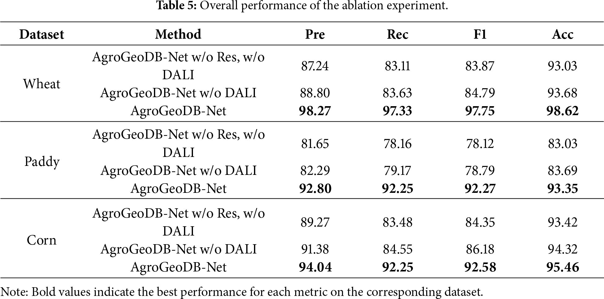
For the paddy dataset, adding the residual shortcut (AgroGeoDB-Net w/o DALI vs. AgroGeoDB-Net w/o Res, w/o DALI) improves accuracy and recall by 0.64% and 1.01%, respectively. With the activation of the DALI module (AgroGeoDB-Net vs. AgroGeoDB-Net w/o DALI), the accuracy and recall further increase by 10.51% and 13.08%, respectively, reinforcing the practicality and robustness of the proposed augmentation strategy in low-density and complex trajectory scenarios.

On the corn dataset, the residual shortcut (AgroGeoDB-Net w/o DALI vs. AgroGeoDB-Net w/o Res, w/o DALI) yields a 2.11% gain in accuracy and a 1.07% gain in recall. After integrating the DALI module (AgroGeoDB-Net vs. AgroGeoDB-Net w/o DALI), an additional improvement of 2.66% in accuracy and 7.70% in recall is achieved. Although the relative gains on this dataset are smaller, which is mainly due to its shorter sampling intervals and the more dispersed distribution of road points, the results still demonstrate that the augmentation strategy remains adaptable under more complex sample structures.

In summary, the experimental results clearly demonstrate that the residual connection enhances the model’s ability to capture long-range temporal dependencies, while the Density-Aware Local Interpolator (DALI) effectively addresses the class imbalance between field and road points in GNSS trajectory data. Combining these two components enables AgroGeoDB-Net to achieve superior classification performance and generalization capability across multiple crop datasets, which confirms the rationality and practical value of the proposed modular design. The overall trends of these improvements are further illustrated in Fig. 6, where the four key metrics (Precision, Recall, F1, and Accuracy) are compared across different module configurations.

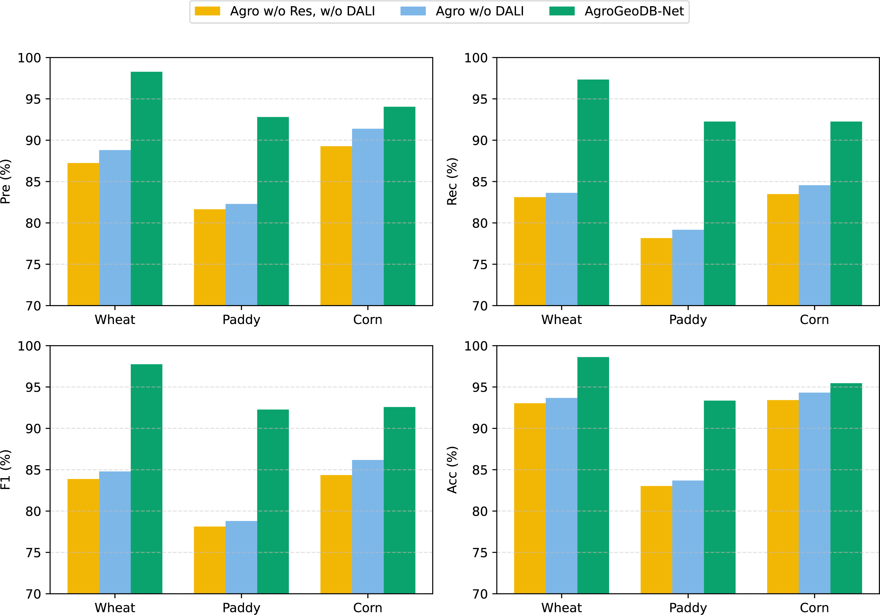
Figure 6: Overall comparison of module contributions across the Wheat, Paddy, and Corn datasets, illustrating the effect of removing the residual shortcut and the DALI module on Precision, Recall, F1-score, and Accuracy.

3.5.2 Class-Wise Analysis

To further quantify the performance contributions of the residual connection and the Density-Aware Local Interpolator (DALI), we conducted ablation experiments separately on the “field points” and “road points” classes. The experimental results are presented in Table 6.

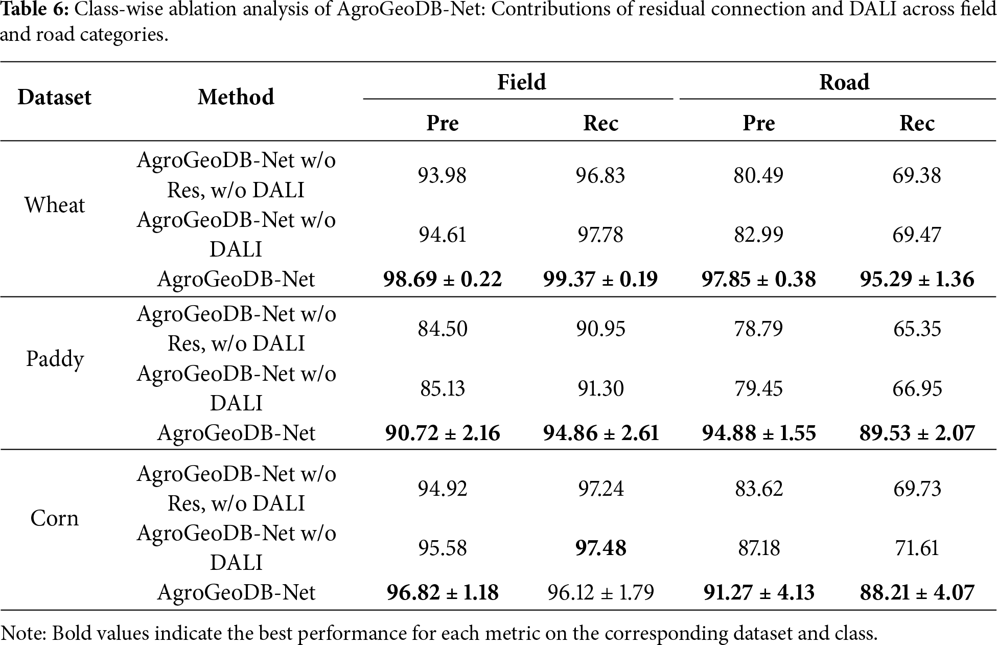
For road points, which constitute the minority class, the two modules exhibit clearly differentiated impacts across all datasets. On the Wheat dataset, enabling the residual shortcut (AgroGeoDB-Net w/o DALI vs. AgroGeoDB-Net w/o Res, w/o DALI) yields small but consistent gains in road precision and recall, indicating improved temporal feature propagation. In contrast, enabling DALI (AgroGeoDB-Net vs. AgroGeoDB-Net w/o DALI) produces substantial improvements, with road precision and recall increasing by large margins and remaining stable across folds, as reflected by the reported standard deviations. A similar pattern is observed on the Paddy dataset, where the residual connection provides modest gains, while DALI leads to pronounced and consistent improvements in both road precision and recall. On the Corn dataset, although overall gains are smaller due to more regular sampling and spatial distribution, DALI still plays the dominant role, yielding notable improvements in road-point recognition and reducing minority-class errors across folds. Overall, these results indicate that DALI is the primary contributor to minority road-point recognition by enriching sparse segments and mitigating class imbalance, while the residual shortcut offers stable but comparatively modest benefits.

For field points, which constitute the majority class, the same qualitative trend holds, albeit with smaller absolute improvements. On the Wheat and Paddy datasets, the residual shortcut consistently improves field-point precision and recall, reflecting its role in stabilising temporal feature flow. Enabling DALI further refines field-point predictions, yielding additional gains when local density patterns are informative. On the Corn dataset, DALI slightly improves field-point precision while introducing a minor reduction in recall, which can be attributed to the more regular spatial layout and shorter sampling interval of corn trajectories, where density cues are less discriminative. Taken together, both modules contribute positively to majority-class performance, with the residual shortcut improving temporal consistency and DALI providing complementary refinement under favourable density conditions.

3.5.3 Confusion Matrix Visualisation

To better understand how different modules affect the classification behaviour of AgroGeoDB-Net, confusion matrices for one representative trajectory from each dataset are visualised in Fig. 7.

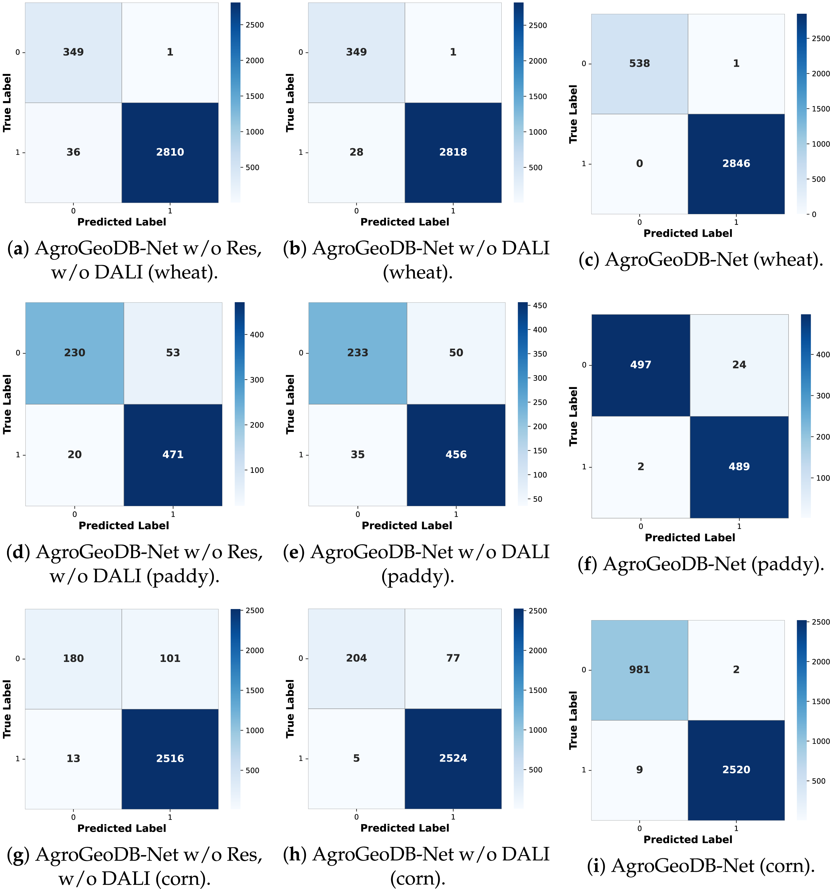
Figure 7: Confusion matrices of three model variants on the wheat, paddy, and corn datasets.

The confusion matrices explicitly report false negatives and false positives for the road class, enabling direct inspection of minority-class behaviour under severe class imbalance. For completeness, we report road-positive precision, recall, F1-score, and balanced accuracy for AgroGeoDB-Net in Appendix C.

A clear trend of improvement appears as the residual shortcut and the Density-Aware Local Interpolator (DALI) are successively enabled. On the wheat dataset, adding the residual shortcut reduces misclassified field points, and enabling DALI leads to perfect classification for that sample. For the paddy dataset, the residual shortcut primarily lowers road-point errors, and activating DALI substantially reduces mistakes in both classes. On the corn dataset, the residual shortcut cuts errors for both road and field points, while DALI sharply decreases road-point errors, despite a slight increase in field-point misclassifications.

These patterns show that the two components work in complementary ways. The residual shortcut helps stabilise temporal feature flow and brings a moderate reduction in errors. DALI plays a more decisive role in correcting mistakes on the minority road class, likely by addressing sample sparsity and ambiguity along road segments. Together, the visualisations clarify how each module strengthens the model’s ability to separate field and road points in GNSS trajectories.

3.6 Model Generalization Capability Evaluation

To assess the generalization capability of AgroGeoDB-Net, we further evaluated the model on two additional agricultural machinery trajectory datasets that were not involved in any stage of training or model development: Harvester and Tractor. The Harvester dataset was collected and organized by our research team, while the Tractor dataset was provided by the Key Laboratory of Agricultural Big Data of the Ministry of Agriculture and Rural Affairs. Detailed dataset statistics are listed in Table 7, and Fig. 8 illustrates the point-count distribution and class imbalance of the two datasets.

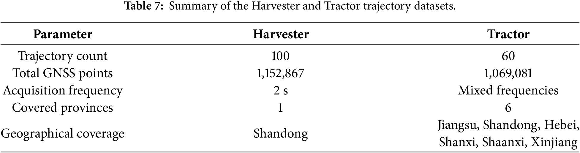
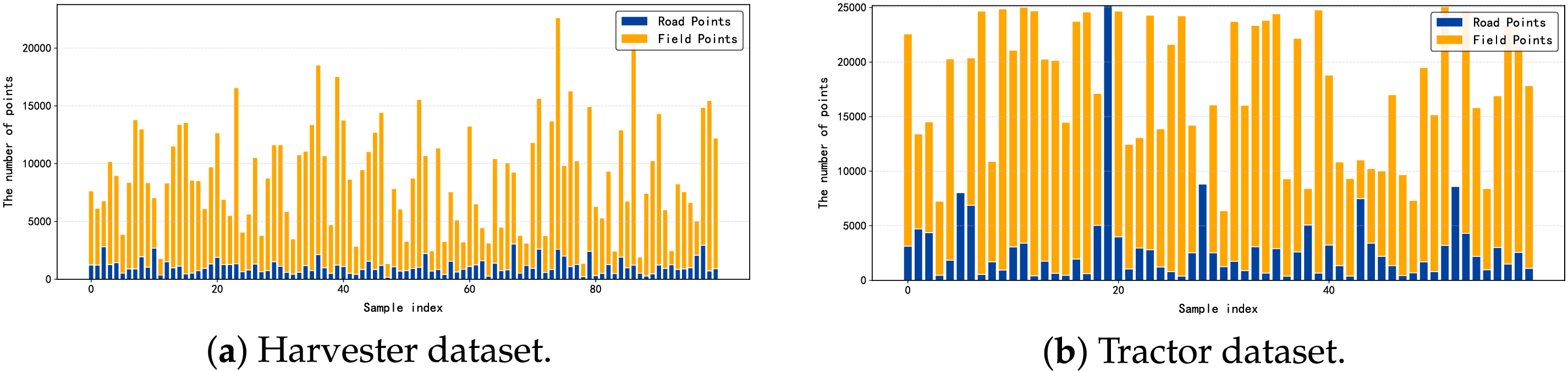
Figure 8: The number and proportion of trajectory points in each sample: (a) Harvester dataset and (b) Tractor dataset. Each bar represents the count and relative percentage of labeled samples, illustrating dataset imbalance between categories.

To ensure a fair and stable assessment, we applied 10-fold cross-validation on both datasets. The results, summarized in Table 8, demonstrate that AgroGeoDB-Net maintains consistently strong performance even when tested on datasets that differ significantly from the training data in crop type, working patterns, sensor sampling frequencies, and geographical regions.

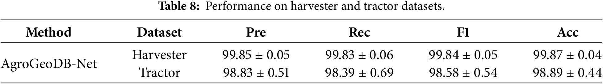
AgroGeoDB-Net maintains high performance on both the Harvester and Tractor datasets. On the Harvester dataset, it achieves consistently high metrics, indicating stable classification under relatively regular operating conditions. For the more diverse Tractor dataset, which spans multiple provinces and exhibits greater variability in operation patterns and sampling characteristics, the model also demonstrates robust performance. To better interpret the unusually strong results observed on these unseen datasets, we further examine their geographic characteristics. As reported in Appendix D, a dataset-level geographic coverage and overlap analysis shows that both the Harvester and Tractor datasets are geographically more concentrated than the multi-region training datasets, with the Harvester dataset exhibiting the most pronounced spatial concentration.

It is worth noting that the GNSS trajectories used in this study represent centreline motion traces and do not explicitly encode physical road width; therefore, variations in actual road width do not directly influence the density-based processing. In addition, although locally straight farmland segments may occur, ultra-long and perfectly straight farmland operations are uncommon in practical agricultural settings due to parcel boundaries and operational patterns. Together with the use of temporal continuity and sequence-level context, these geographic properties provide important context for understanding the observed generalisation behaviour.

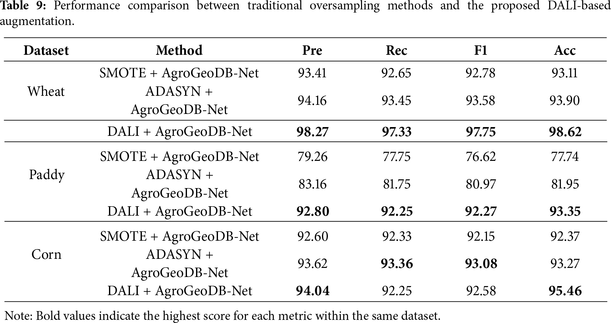
3.7 Comparison with Traditional Oversampling Methods

Ablation results in Section 3.5 show that the Density-Aware Local Interpolator (DALI) yields the largest performance gains for the minority (road) class among the proposed components. To further characterize the nature of this improvement, we compare DALI with two widely used feature-space oversampling methods, SMOTE [25] and ADASYN [26], which do not explicitly account for spatial continuity or geometric constraints.

For a fair comparison, SMOTE and ADASYN are applied to the road class only, while keeping the network architecture and training protocol identical to AgroGeoDB-Net. Table 9 summarises the results on the wheat, paddy, and corn datasets. Overall, ADASYN performs slightly better than SMOTE, but both methods are consistently outperformed by the proposed DALI-based augmentation, particularly on datasets with clearer spatial road structure (wheat and paddy). On the corn dataset, where road trajectories are more dispersed, ADASYN achieves marginally higher recall, while DALI maintains higher precision and accuracy, resulting in comparable or superior overall performance.

To further illustrate qualitative differences, Fig. 9 visualises the augmented road points produced by each method for the same trajectory sample. SMOTE and ADASYN generate synthetic points in feature space without enforcing spatial continuity, which leads to scattered points and geometrically implausible road segments. In contrast, DALI inserts new points along locally coherent road fragments identified by DBSCAN, preserving trajectory continuity and spatial structure. This geometric consistency explains why DALI yields more stable and discriminative improvements, especially for sparse road segments.

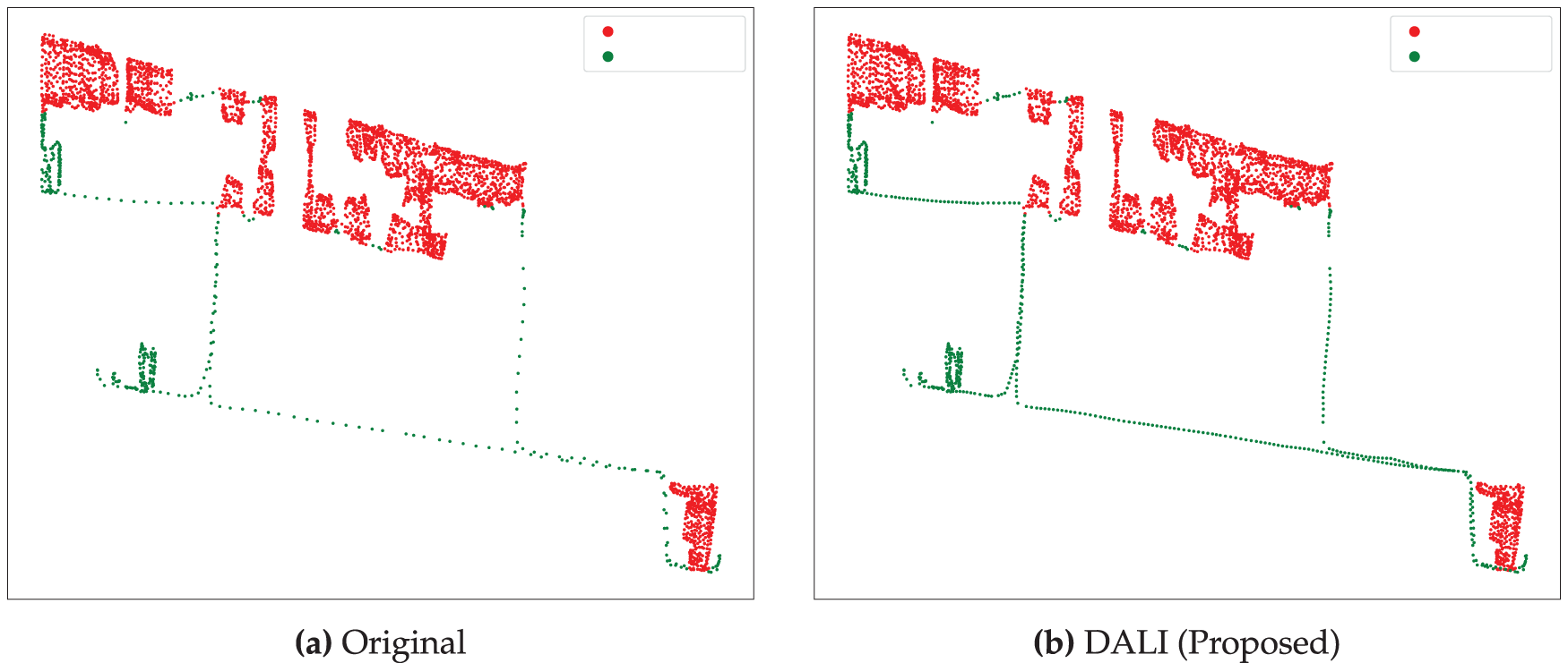
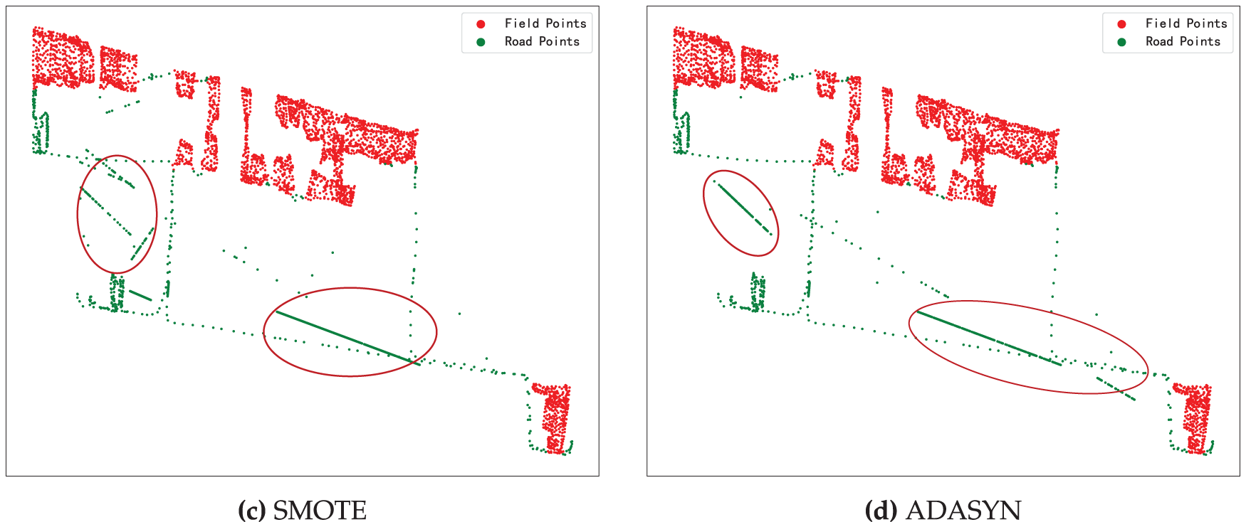
Figure 9: Visualization of road point (Green) augmentation.

4  Conclusions and Future Work

This paper presents AgroGeoDB-Net, a framework for field-road classification of GNSS trajectory data. The framework employs density-aware interpolation to mitigate data imbalance between field and road points, multi-scale descriptors to enrich point-wise features, and a variational encoder with a residual bidirectional LSTM to enhance temporal representation. Together, these components form a coherent pipeline for field–road classification. Experimental results show that AgroGeoDB-Net achieves robust performance across multiple datasets. Ablation studies confirm the contribution of each proposed module, with the density-aware interpolator proving particularly effective in improving recognition of the underrepresented road class. The model also generalizes well, maintaining strong accuracy on the previously unseen Harvester and Tractor datasets under varied geographic and operational conditions.

A current limitation of this work is its strong reliance on fully annotated GNSS trajectory data, despite the fact that large-scale agricultural machinery fleets generate vast amounts of unlabeled traces. Reducing the dependence on manual labeling is therefore essential for wider deployment. Future work will explore label-efficient learning strategies, including self-supervised pretraining and cross-domain adaptation, to improve robustness and transferability across large, heterogeneous agricultural trajectory corpora.

Acknowledgement: The authors would like to thank the support of the Key R&D Program of Shandong Province, the National Natural Science Foundation of China, and the Innovation Capability Enhancement Program for Technology-Based SMEs of Shandong Province.

Funding Statement: This research was supported by the Key R&D Program of Shandong Province, China (Grant No. 2024CXGC010905) and the National Natural Science Foundation of China (Grant Nos. 42201458 and 52575294).

Author Contributions: Methodology, Fengqi Hao and Yawen Hou; Software, Fengqi Hao and Yawen Hou; Formal analysis, Conghui Gao; Writing—original draft, Yawen Hou; Writing—review and editing, Conghui Gao, Jinqiang Bai, Gang Liu, Hoiio Kong and Xiangjun Dong. All authors reviewed and approved the final version of the manuscript.

Availability of Data and Materials: The datasets used in this study are available from public sources. The datasets are publicly available at https://github.com/netcalf/AgroGeoDB-Net.

Ethics Approval: Not applicable.

Conflicts of Interest: The authors declare no conflict of interest.

Appendix A Implementation Details of Trajectory Preprocessing

This appendix consolidates all trajectory preprocessing operations used in this work, providing explicit computational definitions, parameter settings, and unit conventions. All steps described here are implemented deterministically and applied identically to all datasets prior to feature extraction and model training.

Appendix A.1 Duplicate and Redundancy Removal

Two forms of redundancy are removed sequentially. First, duplicate timestamps within the same trajectory are eliminated to ensure a strictly increasing temporal order. Second, duplicate spatial records are removed by identifying repeated tuples (longitude,latitude,speed). After each removal step, indices are reset to preserve trajectory continuity.

Appendix A.2 Geodesic Distance Computation

Point-to-point distances are computed using the haversine formula under a spherical Earth assumption with radius R=6,371,000 m. Given two consecutive points (ϕ1,λ1) and (ϕ2,λ2) in WGS84 latitude and longitude (degrees), the geodesic distance is

d=2Rarctan(a,1−a),a=sin2Δϕ2+cos⁡ϕ1cos⁡ϕ2sin2Δλ2.(A1)

All distances are computed in metres and rounded to two decimal places.

Appendix A.3 Moving-Average Smoothing and Scattered-Point Removal

To suppress isolated noise and GNSS jitter, a causal moving average is applied to the inter-point distance sequence. Given a window size of n=20, the smoothed distance at index i is defined as the mean of the most recent up to n+1 raw distance values.

Trajectory points whose smoothed inter-point distance is less than or equal to 1.0 m are regarded as scattered or stationary noise and removed. This operation eliminates dense micro-fluctuations caused by GNSS drift while preserving genuine low-speed operational motion.

Appendix A.4 Drift-Point Detection and Removal

After initial filtering, a second distance computation is performed on the updated trajectory. Drifting points are identified using a relative-distance consistency rule. Specifically, a point pi is removed if its inter-point distance exceeds six times that of its immediate neighbours, indicating an abrupt and implausible spatial jump. Boundary cases near the start and end of trajectories are handled symmetrically.

This step targets sporadic GNSS outliers without introducing trajectory fragmentation.

Appendix A.5 Output Format and Unit Conventions

After preprocessing, each trajectory point retains the following attributes: timestamp, longitude, latitude, speed, bearing, and semantic label. Among these, longitude, latitude, speed, bearing, and timestamp constitute the input information used for downstream density computation, feature extraction, and model inference, while the semantic label is used exclusively for supervised training and evaluation. All spatial quantities are expressed in metres, angular quantities in degrees, and temporal resolution is preserved as recorded in the original data. The resulting cleaned trajectories are then used for subsequent processing without further modification.

Appendix B Density–Label Relationship Analysis

This appendix provides supplementary empirical evidence for a central premise of the proposed framework, namely that local point density carries informative signals for distinguishing field and road operations. Importantly, all analyses reported here strictly follow the same ε-neighbourhood definition and dataset-fixed DBSCAN parameters as described in Section 2.1.1 of the main text. No additional tuning or alternative density definitions are introduced.

Appendix B.1 Trajectory-Level Density Statistics

For each trajectory point pi, local density is quantified as the number of neighbouring points within its ε-neighbourhood, denoted as Nε(pi). To reduce point-level noise and better reflect operational patterns, we aggregate density statistics at the trajectory level.

Specifically, for each trajectory, we compute (i) the mean and (ii) the median of Nε(pi) separately for field and road points. Figs. A1 and A2 report the dataset-level averages of these trajectory-wise statistics.

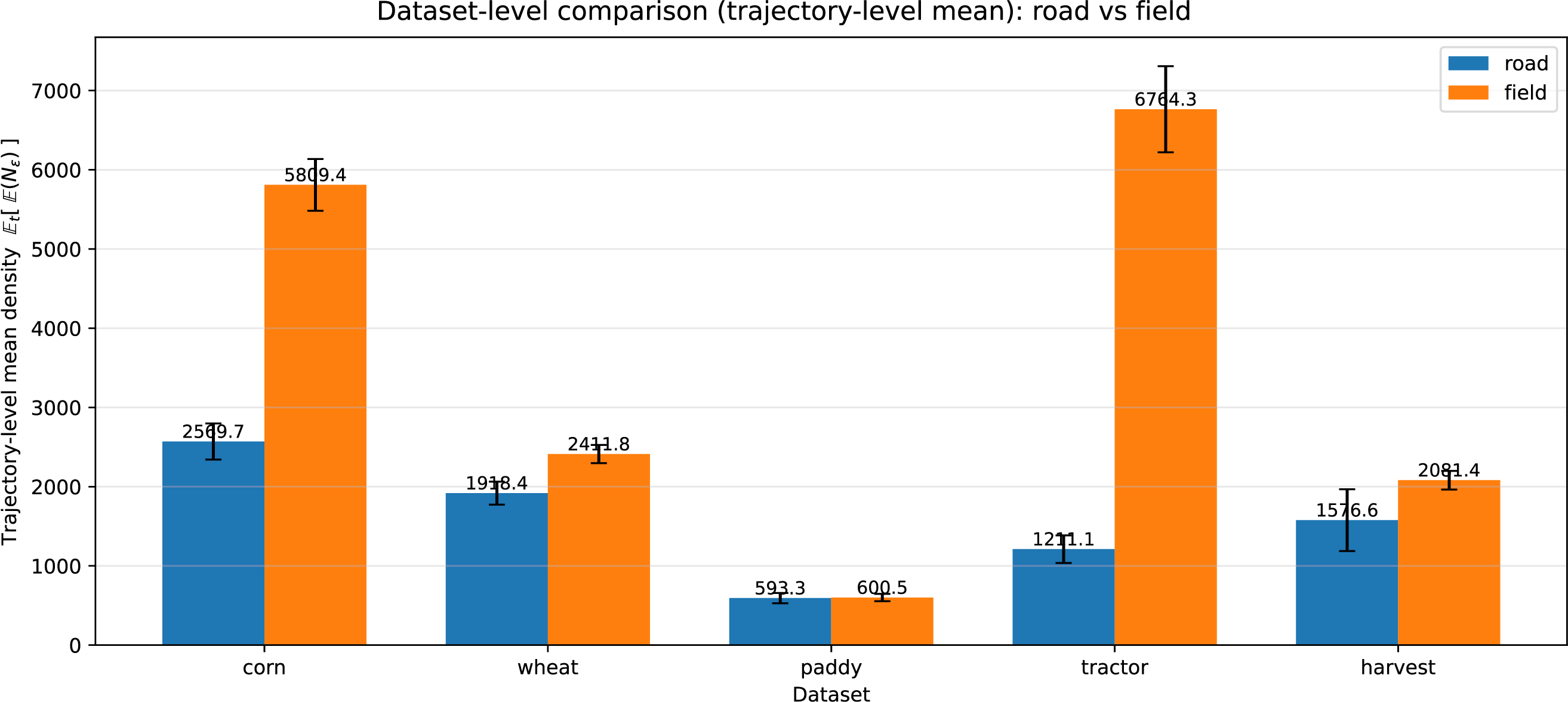
Figure A1: Dataset-level comparison of trajectory-wise mean local density Nε(pi) for field and road operations.

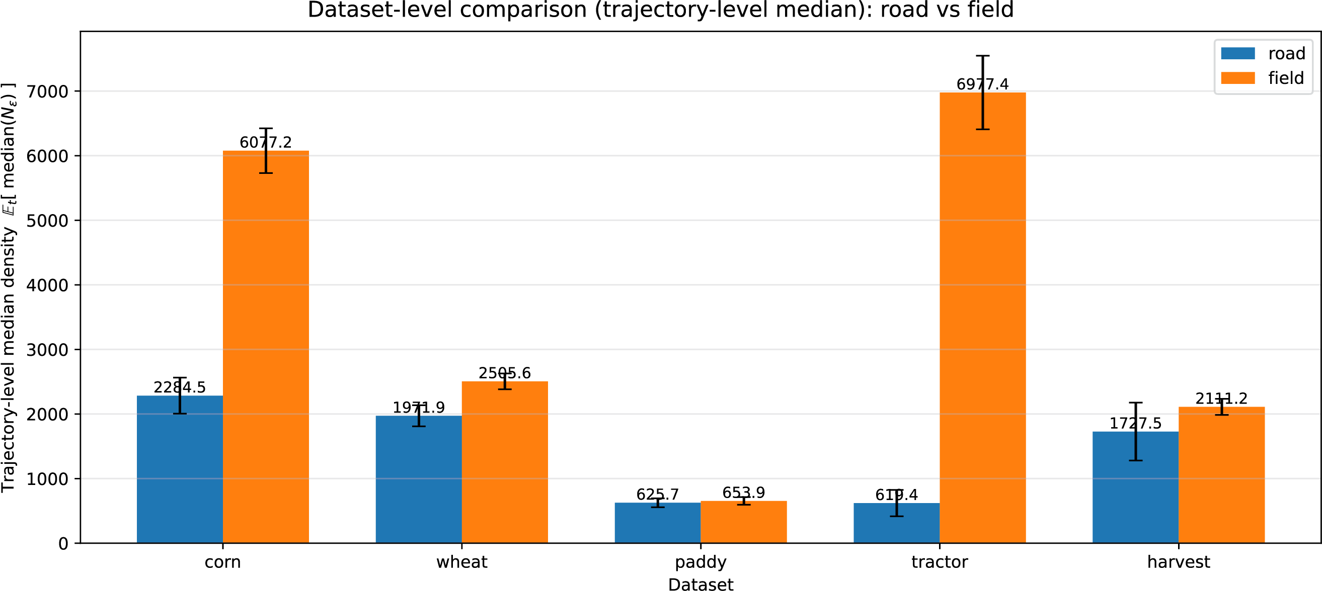
Figure A2: Dataset-level comparison of trajectory-wise median local density Nε(pi) for field and road operations.

Across all datasets, field trajectories consistently exhibit higher average and median neighbourhood density than road trajectories. This reflects the repetitive, low-speed, and spatially confined nature of in-field operations, in contrast to the faster and more spatially sparse characteristics of road travel. These results confirm that, under a consistent ε regime, local density provides a strong statistical cue for field–road discrimination at the dataset level.

Appendix B.2 Limitations and Representative Ambiguity Scenarios

Figs. A1 and A2 validate the density prior at the dataset and trajectory levels under the same neighbourhood scale ε used by our pipeline. We note that ε is critical: overly small values make density dominated by sampling noise, whereas overly large values tend to saturate neighbourhood counts and reduce separability. Therefore, the statistics reported here are computed using the dataset-fixed ε adopted in Section 2.1.1, ensuring a method-consistent validation.

Meanwhile, density does not uniquely determine operational labels at the point level, and a small number of trajectories may violate the prior under trajectory-level aggregation. Two common ambiguity mechanisms are observed. First, temporary road stops or waiting events can create locally dense clusters on roads; this often appears as a tail effect where a few high-density stop points inflate the road mean, while the median remains stable. Second, sparse-field operations under coarse sampling or large parcels may yield relatively low density despite genuine in-field work, weakening density separation.

These observations confirm that density is an informative but imperfect cue. This motivates its use as an inductive bias rather than a deterministic rule, and supports combining density with temporal continuity and geometric context through sequence modelling. The analysis code, trajectory-level statistics, and the counterexample trajectory list have been updated in the public code repository and referenced in the revised manuscript.

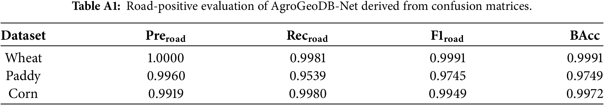
Appendix C Road-Positive Evaluation of AgroGeoDB-Net

This appendix reports road-positive evaluation metrics for AgroGeoDB-Net, derived directly from the confusion matrices shown in Fig. 7. Here, road points are treated as the positive class by swapping the roles of positive and negative labels in the original field-positive confusion matrices. The corresponding quantitative results are summarised in Table A1.

Appendix D Geographic Coverage and Overlap Analysis

This appendix provides supplementary geographic evidence to support the interpretation of the generalisation results reported in the main text. Motivated by leakage-related concerns, we quantify dataset-level geographic coverage and geographic overlap between each dataset and the aggregated training-region footprint. All computations are performed using GNSS coordinates only and do not involve labels or model predictions.

Appendix D.1 Geographic Coverage (Extent)

For each dataset, we compute a dataset-level geographic bounding box from all trajectory points and report its geographic extent. This indicator reflects the overall geographic footprint covered by the dataset and provides a coarse characterisation of geographic concentration vs. multi-region coverage. Fig. A3 compares the geographic extents across the five datasets. The Harvester datasets exhibit substantially smaller geographic coverage than the multi-region datasets, indicating higher geographic concentration.

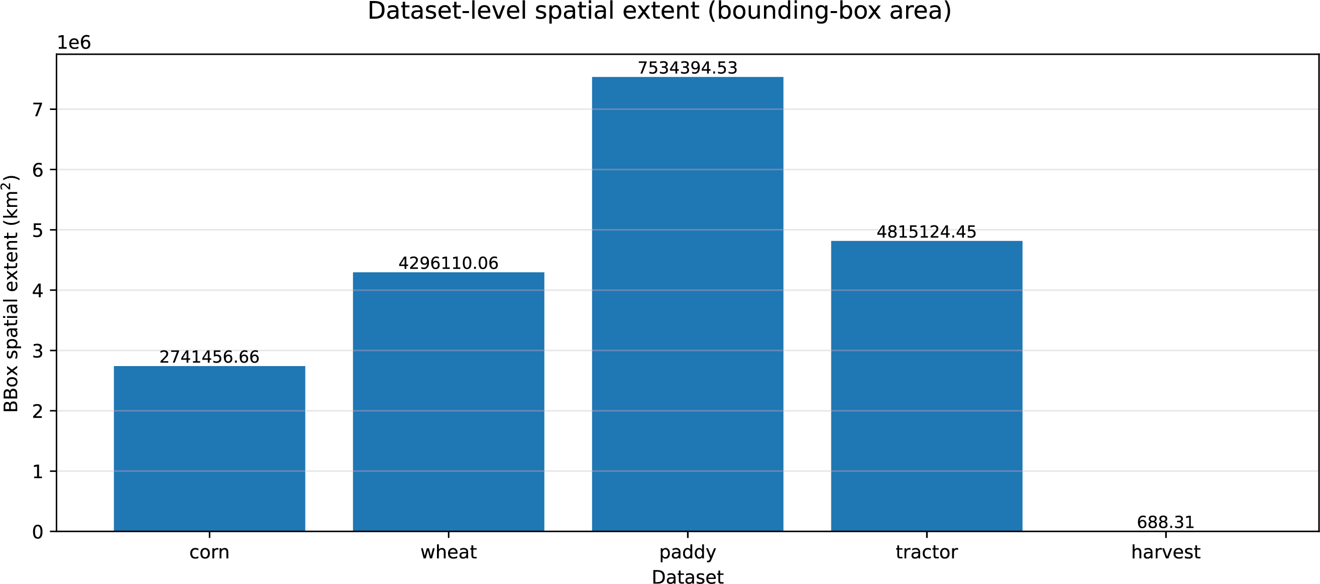
Figure A3: Geographic coverage comparison across datasets, measured by dataset-level bounding-box extent.

Appendix D.2 Geographic Overlap with the Training-Region Footprint

To assess geographic overlap between datasets, we construct an aggregated training-region bounding box using all training datasets and compute the geographic overlap between each dataset and this training-region footprint. The overlap is quantified in terms of overlap area and its ratio with respect to the dataset’s own geographic footprint.

Fig. A4 reports the resulting geographic overlap statistics. The Harvester dataset exhibits the highest degree of geographic concentration, with trajectories confined to a narrow region. The Tractor dataset shows a similar but less pronounced concentration pattern, while the remaining datasets cover substantially broader geographic extents.

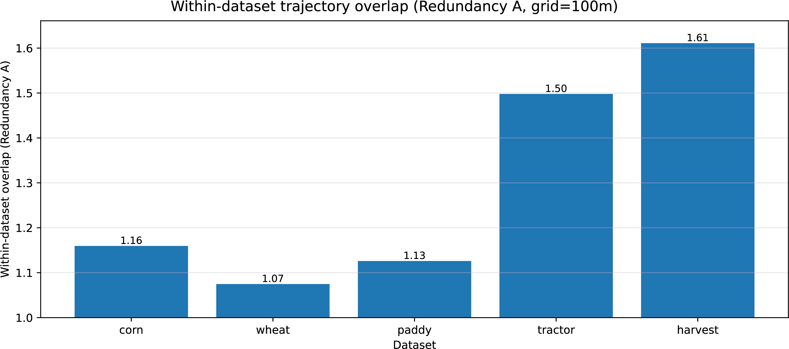
Figure A4: Geographic overlap between each dataset and the aggregated training-region footprint.

References

1. Wu C, Li D, Zhang X, Pan J, Quan L, Yang L, et al. China’s agricultural machinery operation big data system. Comput Electron Agric. 2023;205:107594. doi:10.1016/j.compag.2022.107594. [Google Scholar] [CrossRef]

2. Shi M, Paudel KP, Chen F. Mechanization and efficiency in rice production in China. J Integrat Agricul. 2021;20(7):1996–2008. doi:10.1016/s2095-3119(20)63439-6. [Google Scholar] [CrossRef]

3. Zheng Y, Li Q, Chen Y, Xie X, Ma WY. Understanding mobility based on GPS data. In: Proceedings of the 10th International Conference on Ubiquitous Computing; 2008 Sep 21–4; Seoul, Republic of Korea. p. 312–21. [Google Scholar]

4. Zheng Y, Zhang L, Xie X, Ma WY. Mining interesting locations and travel sequences from GPS trajectories. In: Proceedings of the 18th International Conference on World Wide Web; 2009 Apr 20–24; Madrid, Spain. p. 791–800. [Google Scholar]

5. Zheng Y, Zhou X. Computing with spatial trajectories. New York, NY, USA: Springer Science & Business Media; 2011. [Google Scholar]

6. Zhang X, Cao M, Gong Y, Wu X, Dong X, Guo Y, et al. Enhancing urban flow prediction via mutual reinforcement with multiscale regional information. Neural Netw. 2025;182(3):106900. doi:10.1016/j.neunet.2024.106900. [Google Scholar] [PubMed] [CrossRef]

7. Chen W, Liang Y, Zhu Y, Chang Y, Luo K, Wen H, et al. Deep learning for trajectory data management and mining: a survey and beyond. arXiv:2403.14151. 2024. [Google Scholar]

8. Gao Q, Zhou F, Zhang K, Trajcevski G, Luo X, Zhang F. Identifying human mobility via trajectory embeddings. In: Proceedings of the Twenty-Sixth International Joint Conference on Artificial Intelligence (IJCAI-17); 2017 Aug 19–25; Melbourne, VIC, Australia. p. 1689–95. [Google Scholar]

9. Zhou F, Gao Q, Trajcevski G, Zhang K, Zhong T, Zhang F. Trajectory-user linking via variational autoencoder. In: Proceedings of the Twenty-Seventh International Joint Conference on Artificial Intelligence (IJCAI-18); 2018 Jul 13–19; Stockholm, Sweden. p. 3212–8. [Google Scholar]

10. Chen W, Huang C, Yu Y, Jiang Y, Dong J. Trajectory-user linking via hierarchical spatio-temporal attention networks. ACM Trans Knowl Disc Data. 2024;18(4):1–22. doi:10.1145/3635718. [Google Scholar] [CrossRef]

11. Wang X, Yang D, Li L, Li C, Lian J, Zhao J, et al. Robust trajectory prediction based on efficient fusion of heterogeneous information. IEEE Trans Vehic Technol. 2026;75(1):114–29. doi:10.1109/tvt.2025.3591243. [Google Scholar] [CrossRef]

12. Chen Y, Zhang X, Wu C, Li G. Field-road trajectory segmentation for agricultural machinery based on direction distribution. Comput Electron Agric. 2021;186:106180. doi:10.1016/j.compag.2021.106180. [Google Scholar] [CrossRef]

13. Ester M, Kriegel HP, Sander J, Xu X. A density-based algorithm for discovering clusters in large spatial databases with noise. In: KDD’96: Proceedings of the Second International Conference on Knowledge Discovery and Data Mining. Palo Alto, CA, USA: AAAI Press; 1996. Vol. 96, p. 226–31. [Google Scholar]

14. Poteko J, Eder D, Noack PO. Identifying operation modes of agricultural vehicles based on GNSS measurements. Comput Electron Agric. 2021;185(3):106105. doi:10.1016/j.compag.2021.106105. [Google Scholar] [CrossRef]

15. Bian C, Bai J, Cheng G, Hao F, Zhao X. ConvTEBiLSTM: a neural network fusing local and global trajectory features for field-road mode classification. ISPRS Int J Geo Inf. 2024;13(3):90. doi:10.3390/ijgi13030090. [Google Scholar] [CrossRef]

16. Luo W, Feng Y, Zhao C, Xu J, Shao X, Xu L. A BiLSTM-based joint attention model for vehicle trajectory prediction. J Supercomput. 2025;82(1):11. doi:10.1007/s11227-025-08144-3. [Google Scholar] [CrossRef]

17. Zhou S, Li J, Wang H, Shang S, Han P. GRLSTM: trajectory similarity computation with graph-based residual LSTM. In: Proceedings of the AAAI Conference on Artificial Intelligence. Palo Alto, CA, USA: AAAI Press; 2023. Vol. 37, p. 4972–80. [Google Scholar]

18. Hao F, Zhao X, Bian C, Kong H, Dong X, Bai J. VEBiLSTM: a neural network for field-road classification using enhanced spatiotemporal features. In: International Conference on Neural Information Processing. Cham, Switzerland: Springer; 2024. p. 245–58. [Google Scholar]

19. Chen Y, Quan L, Zhang X, Zhou K, Wu C. Field-road classification for GNSS recordings of agricultural machinery using pixel-level visual features. Comput Electron Agric. 2023;210:107937. doi:10.1016/j.compag.2023.107937. [Google Scholar] [CrossRef]

20. Zhai W, Chen L, Liu J, Guo Z, Qian Q, Pan J, et al. Dual-domain Context-aware network in time series classification for identifying agricultural machinery trajectory operation mode. Smart Agricult Technol. 2025;13(4):101774. doi:10.1016/j.atech.2025.101774. [Google Scholar] [CrossRef]

21. Hou Y, Hao F, Bai J, Gao C, Ding Q, Kong H. VE-ResBiLSTM: a deep spatiotemporal model for field-road classification with DBSCAN-based data augmentation. In: International Conference on Intelligent Computing. Cham, Switzerland: Springer; 2025. p. 199–212. [Google Scholar]

22. Campello RJGB, Moulavi D, Sander J. Density-based clustering based on hierarchical density estimates. ACM Trans Knowl Discov Data. 2013;10(1):1–51. [Google Scholar]

23. Schubert E, Sander J, Ester M, Kriegel HP, Xu X. DBSCAN revisited, revisited: why and how you should (still) use DBSCAN. ACM Trans Database Syst. 2017;42(3):19:1–21. doi:10.1145/3068335. [Google Scholar] [CrossRef]

24. Chen Y, Li G, Zhang X, Jia J, Zhou K, Wu C. Identifying field and road modes of agricultural Machinery based on GNSS Recordings: a graph convolutional neural network approach. Comput Electron Agric. 2022;198(1):107082. doi:10.1016/j.compag.2022.107082. [Google Scholar] [CrossRef]

25. Chawla NV, Bowyer KW, Hall LO, Kegelmeyer WP. SMOTE: synthetic minority over-sampling technique. J Artif Intell Res. 2002;16:321–57. doi:10.1613/jair.953. [Google Scholar] [CrossRef]

26. He H, Bai Y, Garcia EA, Li S. ADASYN: adaptive synthetic sampling approach for imbalanced learning. In: 2008 IEEE International Joint Conference on Neural Networks (IEEE World Congress on Computational Intelligence). Piscataway, NJ, USA: IEEE; 2008. p. 1322–8. [Google Scholar]