High-Resolution UAV Image Classification of Land Use and Land Cover Based on CNN Architecture Optimization

1  Introduction

Land use and land cover (LULC) can be broadly classified into two interrelated domains: land cover and land use [1]. land use describes how land is utilized and managed by humans, reflecting the transformation of natural ecosystems into artificial or modified systems. This process is shaped by a complex interplay of natural conditions, economic activities, and social factors. In contrast, Land cover refers to the physical and biological characteristics present on the Earth’s surface, including both natural and human-made features that constitute surface cover. Typical examples include forests, grasslands, croplands, bare soil, and roads [2]. Of the various sources of remote sensing images, satellites are among the most frequently used for surveying and mapping LULC. High-quality and high-resolution satellite images provide detailed spatial information. Although recent satellite platforms (e.g., GeoEye, IKONOS, QuickBird, and Worldview) have achieved submeter spatial resolution, such platforms are expensive. In addition, satellite images often have low temporal resolution (cannot be collected in the same area at different time points) and are susceptible to atmospheric conditions, such as clouds and smog. Although images obtained by manned aircraft can overcome the temporal- and spatial-resolution-related limitations of satellite images, using manned aircraft to obtain aerial images is expensive, requires well-trained pilots, and is dependent on weather conditions [3].

An unmanned aerial vehicle (UAV) is an aircraft equipped with sensors and devices such as optical cameras, multispectral or hyperspectral cameras, LiDAR systems, global positioning systems (GPSs), and flight control devices. The commercial success of UAVs, due largely to their low price and ease of control, has led to new opportunities in remote sensing research. In contrast to satellites, UAVs can fly at low altitudes and can help researchers obtain detailed information by collecting images with high spatiotemporal resolution, some of which have a spatial resolution of <1 dm [4]. Because they can obtain images with high spatial resolution and are low-cost, UAVs are well suited for mapping LULC [5]. Additionally, UAVs can shoot close-range images or conduct LULC telemetry within a specified area within a short time, which is difficult to achieve using aerial photogrammetry or the fixed-orbit satellite mode of manned aircraft. The high cost of aerial and satellite imaging platforms is another obstacle to their use. Overall, remote sensing images collected using UAVs are superior to those collected using manned aircraft and satellites because of the maneuverability, convenience, cost-effectiveness, safety, and efficiency of UAVs as well as the ability of UAVs to capture high-quality images.

Standard methods that use various types of satellite images (spectral and spatial resolution) are not suitable for LULC mapping; therefore, researchers have been exploring the use of high-resolution UAV images for LULC mapping as an alternative. High-resolution remote sensing images are considered ideal for LULC classification [6]. Extracting LULC information usually requires high-spatial-resolution data for digital processing [7]. A very high image resolution facilitates the extraction of geometric and contextual features from images for detailed LULC classification [8]. The resolutions of UAV images are generally higher than those of satellite images [9]. However, traditional LULC classification methods operate at the pixel level and involve evaluating the geometric, textural, and contextual features around each pixel, which makes them unsuitable for LU classification based on high-spatial-resolution images [10]. Detailed information regarding an object may increase the complexity of the within-class texture, often leading to misclassification [11]. Additionally, the detail in high-resolution images can easily lead to excessive fragmentation in pixel classification results and produce a salt-and-pepper effect.

The pixel-based method involves classifying each single pixel into a specific LULC class on the basis of the spectral reflectance of the pixel and disregarding neighboring pixels [12]. This method uses gray values to classify individual pixels but ignores ground objects with spatial characteristics. Therefore, a pixel-level method that relies only on spectral characteristics can classify LULC but is insufficient for distinguishing between LULC images corresponding to multiple types of LULC [13]. However, UAV image researchers often use object-based image analysis (OBIA) methods rather than traditional pixel-based LULC classification methods [14]. OBIA methods use image segmentation to divide image objects into nonoverlapping regions, ensuring that each region is homogeneous according to a certain reoccurring feature and that the union of neighboring regions is nonhomogeneous [15]. OBIA methods are based on the relatively uniform objects composed of similar pixel values throughout an entire image and are used to classify LULC according to the physical properties (e.g., spectrum, texture, and shape) of ground components [16]. The resolution of UAV images has reached an unprecedented level, and OBIA methods often reveal the difficulty in achieving proper image segmentation because when objects vary considerably in both scale and size, shapes and textures may be insufficient for distinguishing among them.

With the increase in ground resolution from meter level to centimeter level, converting pixel-based methods to object-based methods has emerged as a challenge; the problems associated with method conversion are still being actively researched [17]. The training of powerful classifiers employing both pixel- and object-level classification methods relies on the aggregation of extracted spectral, textural, and geometric features to model images from the bottom up [18]. However, pixel- and object-level LULC classification methods are based on shallow architecture. Such methods cannot be used for classification based on the fine features of complex LULC images and are inaccurate when used for many practical applications. Because LULC images are complex, LULC classification methods should be able to extract numerous features and select a detailed subset to yield satisfactory classification results. Deep learning methods can be used to reduce the difficulty and complexity of feature extraction and LULC classification.

Deep learning is the process of obtaining high-level abstract features from data by using mathematical models to achieve high accuracy in the classification and detection of objects. Various neural network models have been proposed; among them, convolutional neural networks (CNNs) are the most common. Researchers have made considerable progress in using CNNs for image recognition, and CNNs are widely used and achieve high accuracy in LULC classification [19,20]. Object-oriented approaches involve lengthy image segmentation and image object feature calculation processes, whereas CNN-based approaches do not involve these two processes and are therefore more efficient for LULC classification [21]. In contrast to pixel- and object-based LULC classification methods, CNNs can be used to extract high-level abstract features from images and exhibit excellent performance in detecting LULC. Such CNN-based multilayer perceptron architectures can extract highly discriminative features and intricate patterns, demonstrating improved LULC classification performance compared with conventional classification approaches [22,23].

Researchers have made significant progress in the application of remote sensing imagery for land use and land cover (LULC) detection, driven by advancements in image resolution, computer vision, and classification algorithms. Recent deep learning approaches, particularly CNNs, have achieved remarkable performance in image classification tasks. More recently, transformer-based architectures, such as the Hybrid Lightweight Transformer, have been incorporated into hybrid CNN–Transformer models (e.g., HybridATNet [24]) and demonstrated competitive or even superior performance by effectively capturing both local and global feature representations. The outstanding performance of CNNs in computer vision tasks—such as object detection, visual recognition, and image classification—can be attributed to their strong capability to detect and represent shapes, textures, and structures, including small buildings, that are often indistinguishable in medium-resolution imagery [25]. Consequently, CNNs have become effective tools for detecting and classifying LULC features in high-resolution images, overcoming the limitations of traditional pixel-based and object-based classification methods. Therefore, in this study, a CNN model was developed and optimized to detect and classify various LULC types using high-resolution UAV imagery.

The primary objective of this study is to systematically investigate the impact of CNN architectural configurations and hyperparameter adjustments, including kernel size, network depth, dropout, batch normalization, and data augmentation, on the classification performance of UAV-based LULC imagery. Rather than benchmarking against external state-of-the-art models, this work emphasizes understanding how internal design choices influence classification accuracy, overfitting behavior, and generalization performance under controlled experimental conditions. Accordingly, the main contribution of this study lies in providing systematic empirical insights into CNN design for UAV-based LULC classification under limited training data conditions. Instead of proposing a novel deep learning architecture, this research analyzes how key architectural and regularization strategies affect model performance and robustness.

Although modern pretrained architectures (such as ResNet and EfficientNet) have demonstrated strong performance on large-scale natural image datasets, their effectiveness typically depends on extensive training data and transfer learning assumptions that may not fully align with domain-specific UAV imagery. Therefore, a lightweight custom CNN is adopted to enable controlled experimentation, reduced model complexity, and transparent evaluation of architectural and hyperparameter effects. This design choice facilitates fair and interpretable comparisons across multiple configurations and supports the identification of an optimized CNN setting tailored to high-resolution UAV-based LULC classification.

2  Research Methods and Materials

2.1 Convolutional Neural Network (CNN)

In deep learning, a CNN is a type of artificial neural network (ANN) in which features are learned hierarchically from training data. CNNs can be used to adjust the weights of training data and automatically generalize, optimize, and simplify parameters to facilitate feature differentiation and extraction [26]. A CNN consists of one or more convolutional, pooling, or fully connected layers and can produce detection results for images or object classes through feature learning. Because a CNN has two more convolutional and pooling layers than a traditional ANN does, a CNN can be used to perceive image details rather than to extract pure data for computation. The input image data usually includes three-dimensional data, such as horizontal, vertical, and color channels. However, the input data of a traditional ANN must be one-dimensional; therefore, traditional ANNs ignore the shapes of objects and lose some essential spatial data. The underlying architecture of a CNN comprises a series of alternating convolutional and pooling layers that are connected and generalize features into depth and abstract representations. A fully connected layer classifies images on the basis of their final labels.

2.1.1 Convolutional Layer

The input of each convolutional layer is an m × m × 3 RGB image, where m × m is the size of the input image and 3 is the number of image channels. The convolutional layer has k filters with a size of n × n × 3, and the size of n × n is smaller than the size of the image (n < m). Each convolutional filter comprises a smaller matrix of values that can be used to separate significant image features when the filter is applied to larger images [27]. The convolutional layer multiplies the matrix values of the filter by the pixel values of the image and adds a deviation value (b) to generate a feature map with a size of l × l × k; k feature maps are generated after convolution. Yi, the ith output feature map, can be calculated using Eq. (1), where Wi is the ith filter and X is the input image. Each position in the input image is assigned a value; when the filter slides over all the positions, a set of matrix values (a feature map) is generated (Fig. 1). Several feature maps with different functions may be present in each convolutional layer. Therefore, filters can be regarded as feature identifiers, which are used to extract various features from images. The more filters are present, the greater the depth of the feature map is, and the easier the content of the input image can be identified. Convolution is performed in the second dimension to extract the contextual spatial features required to classify images.

Yi=Wi×X+b(1)

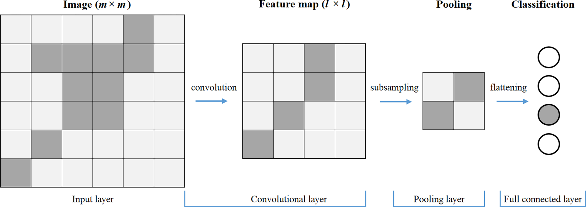
Figure 1: Image feature extraction in CNN.

Each convolutional layer includes an activation function to introduce nonlinearity and increase the feature space that the network can learn. One typical activation function is the rectified linear unit (ReLU) activation function, which is characterized by rapid convergence and simple gradient calculation. The main limitation of the ReLU activation function is that its minimum output value is zero. It can output any nonnegative real value, as expressed in Eq. (2), where x and y are the input and output of the ReLU activation layer, respectively.

y=max(0,x)={xifx>00ifx≤0(2)

The derivative (gradient) of the ReLU activation function is defined as:

dydx={1ifx>00ifx<0(3)

Specifically, the gradient is 1 when the input is positive (x > 0) and 0 when the input is negative (x < 0). This ensures simple gradient calculation and helps mitigate the vanishing gradient problem. The feature map is then generated using the results. Each point on the feature map can be regarded as a feature of the corresponding region in the original image.

2.1.2 Pooling Layer

The pooling layer reduces the spatial dimensionality (length and width) of the input image. However, the RGB depth remains unchanged, and the key features of the feature map are preserved, which can minimize computational costs and control overfitting. In addition, the pooling layer makes the CNN translation locally invariant and focuses only on whether a feature appears or not, rather than on the specific location where a feature appears. Pooling layers can include three operations: average, max, and stochastic pooling. The size of an image neighborhood may contribute to variance in estimates and inaccuracy during the feature extraction process; in such cases, average pooling can be used to minimize error and retain image background information. Max pooling can be used to reduce error in the convolutional layer parameters and highlight features, such as texture. Stochastic pooling can be used to assign a probability to each pixel value and perform probability-based sampling. All pooling layers in the models employ max pooling, which computes the maximum pixel value within a region (while ignoring the remaining values) for subsampling and parameter reduction, thereby facilitating the extraction of abstract features.

2.1.3 Fully Connected Layer

Each feature map output from the convolutional layers represents a specific feature of the input image. As the network depth increases, increasingly abstract and high-level features are learned. A fully connected layer is employed to integrate these extracted features and perform final classification. For the four-class LULC classification task considered in this study, the fully connected layer adopts a softmax activation function to produce a normalized probability distribution over the four mutually exclusive land-use and land-cover classes. The training process uses backpropagation, in which model parameters are iteratively updated after forward propagation and loss computation. To ensure consistency with the softmax-based multi-class classification setting, the categorical cross-entropy loss function is used. This loss function measures the discrepancy between the predicted class probability distribution and the ground truth labels and is widely adopted in deep learning applications. It is defined as:

Categorical cross−entropy=−1s∑i=1s∑c=1sgi,clog⁡(pi,c),(4)

where s denotes the total number of training samples, c is the number of classes (c = 4), pi,c represents the predicted probability of sample i belonging to class c, and gi,c is the corresponding one-hot encoded ground truth label. In the implementation, categorical cross-entropy loss is employed with a softmax output layer (from_logits = False), ensuring consistency between the mathematical formulation and the TensorFlow training configuration for the four-class classification task.

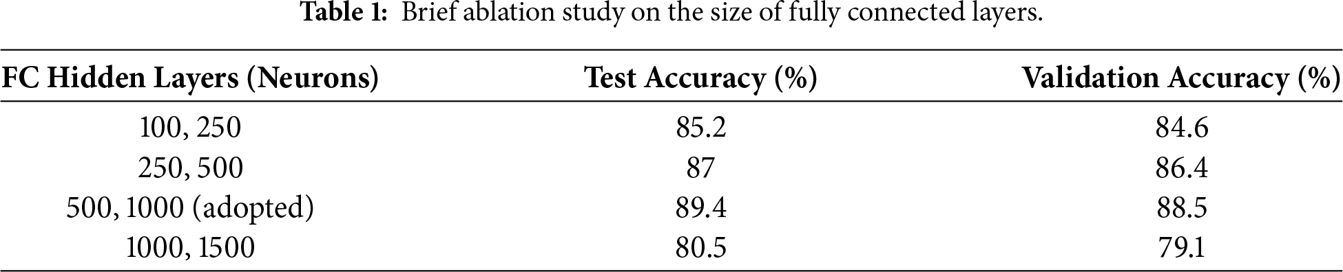
To justify the design of the fully connected (FC) layers, a brief ablation analysis was conducted prior to the main experiments. In this analysis, the number of neurons in the FC layers was varied while keeping all convolutional layers and training settings, including the optimizer, learning rate, batch size, and number of epochs, unchanged. The objective was to assess the impact of FC layer dimensionality on classification performance and to avoid underfitting caused by insufficient model capacity.

The ablation results (Table 1) indicate that both overly compact and excessively large fully connected (FC) layer configurations lead to reduced validation and test accuracy. When the FC layers are too small, the model lacks sufficient capacity to effectively integrate high-level features extracted by the convolutional layers, resulting in underfitting. Conversely, increasing the FC dimensionality beyond a certain point degrades performance, likely due to increased model complexity and overfitting under limited data conditions. Based on this analysis, the FC configuration with 500 and 1000 neurons was selected as a balanced design that achieves the best trade-off between representational capacity and generalization, and was therefore adopted in all subsequent experiments.

2.1.4 Hyperparameters

Because of the complexity of high-resolution images, such images must be used to train networks with multiple layers. As the network deepens, model training becomes more difficult, and convergence slows. Although stochastic gradient descent is simple and efficient in training deep networks, it requires manual adjustment of hyperparameters. During the training process, researchers can monitor the loss and accuracy on the validation set to determine whether any hyperparameters must be adjusted [28]. The optimal parameters are determined through the evaluation of the accuracy of multiple trained networks on validation data.

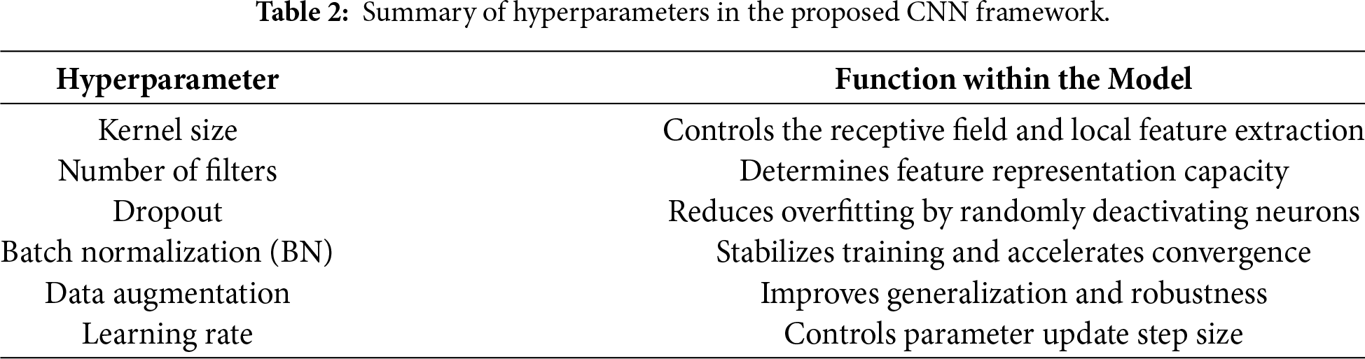
The learning rate of a network refers to the rate at which the parameters of a model are adjusted using gradient descent; higher learning rates correspond to greater updates in weights and, in turn, faster learning, causing the model to require less time to converge to the optimal weight. When the learning rate is too high, the frequency of parameter updates becomes excessive, contributing to the risk of oscillation and nonconvergence. Batch normalization (BN) refers to the normalization of the input data in each layer of a network (to obtain a mean value of 0 with a standard deviation of 1) and can reduce the variability of each sample in a batch. BN can accelerate deep network training and prevent internal covariate shifting [29]. Moreover, BN can desensitize a model to the network parameters, stabilize network learning by simplifying the parameter adjustment process, and prevent vanishing gradients during model training, thus making the use of high learning rates more feasible. In addition, dropout and data augmentation are also crucial to the results of model training. During the training process, various parameter initialization methods should be used to accelerate model convergence. Table 2 summarizes the key hyperparameters used in this study and their respective function in the CNN framework.

2.2 Study Area and Image Data

The time of day, season, lighting conditions, and weather can significantly impact the quality and consistency of remotely sensed imagery, and consequently, model performance. Variations in solar angle throughout the day can lead to differences in illumination, shadow length, and contrast, potentially altering the spectral and textural appearance of land cover features. Seasonal changes affect vegetation phenology, surface moisture, and ground cover, introducing further variability in class characteristics. Additionally, weather conditions—such as cloud cover, haze, or precipitation—can reduce image clarity and introduce noise, complicating feature extraction and classification. In this study, all images were acquired under consistent, cloud-free conditions during a fixed time window to minimize such effects.

All imagery was captured using a DJI Phantom-3 UAV equipped with a 12-megapixel RGB sensor and flown at a fixed altitude of 60 m above ground level. The flight altitude remained consistent throughout all image acquisitions to ensure uniform spatial resolution across the dataset. Images were collected during daytime hours, typically between 9:00 a.m. and 11:00 a.m., under stable and clear weather conditions to minimize variations in illumination and atmospheric effects. These parameters were held constant for all flights to reduce environmental variability.

The UAV did not hover for extended periods at each location; instead, it followed predefined flight paths that covered the study area in a systematic grid pattern, capturing nadir (downward-looking) images at regular intervals. The number of images in the final dataset (800) is relatively small because images were manually selected and cropped to represent clear and unambiguous examples of four targeted land cover categories. This deliberate curation ensured high-quality labeling but limited the overall dataset size. The study area was also spatially constrained, reflecting a practical scenario for urban land cover mapping with limited UAV flight time and data storage. In summary, all images were acquired at a uniform altitude and within a narrow time window under consistent, cloud-free weather conditions, ensuring data homogeneity and controlling for potential confounding variables.

The images were captured in Fengshan District, located in the southern part of Kaohsiung City, Taiwan. The LULC types in the study area included trees and grasslands (natural) as well as buildings and roads (man-made). The UAV imagery was acquired with a spatial resolution (ground sampling distance) of approximately 0.02 m/pixel. As training a CNN model requires a substantial amount of image data, the UAV imagery was cropped into four LULC categories: trees, grasslands, buildings, and roads. A total of 800 image tiles were manually labeled and organized into datasets corresponding to these four LULC classes (Fig. 2). The UAV images were partitioned into 800 non-overlapping tiles, each with a fixed size of 150 × 150 pixels, which served as inputs to the CNN models. This tile size was selected to balance spatial detail preservation and computational efficiency while ensuring uniform input dimensions across all experiments.

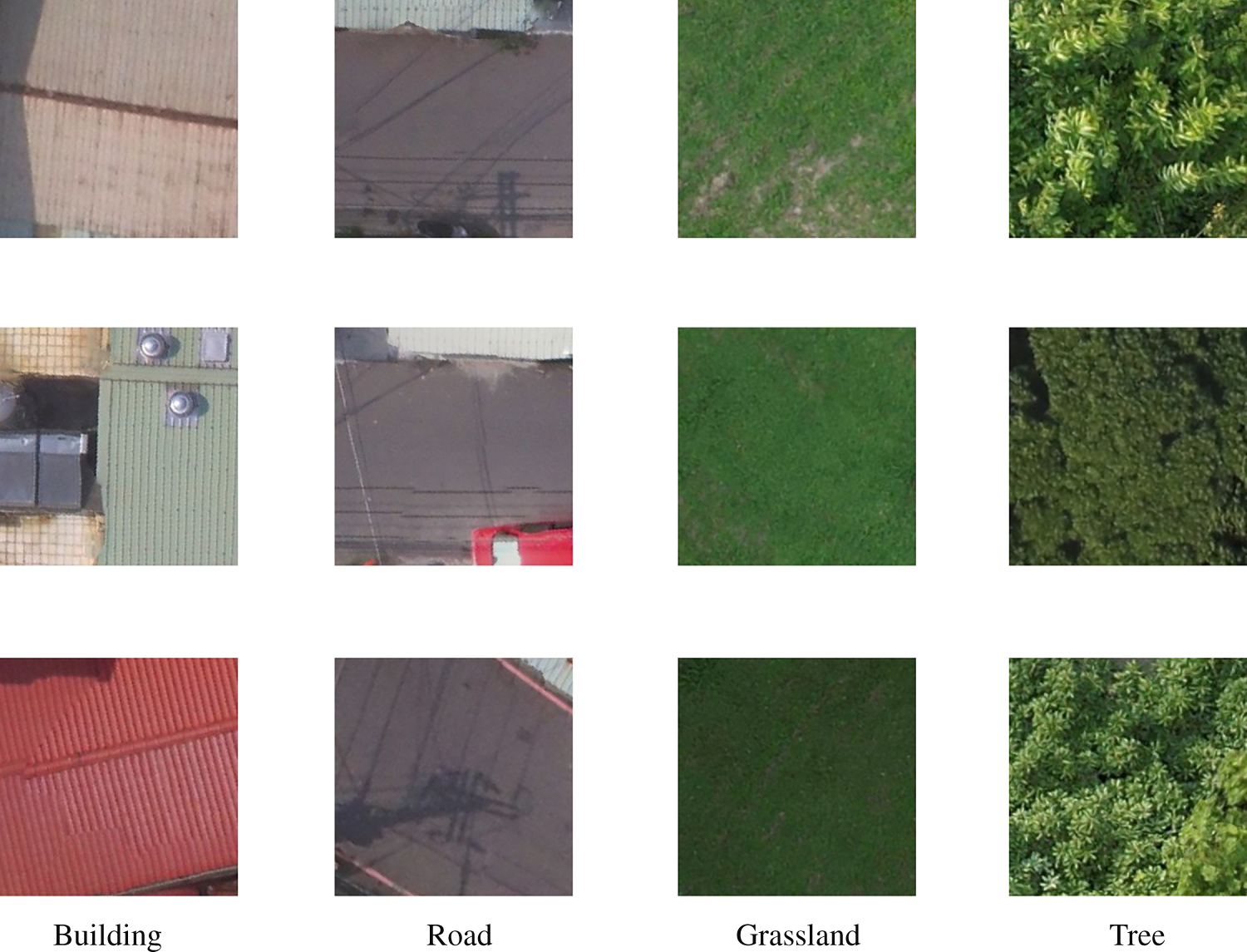
Figure 2: Images of four types of land cover in the study area.

Given the relatively limited dataset size, adopting k-fold cross-validation would reduce the number of samples available for training in each fold, which may affect training stability and learning consistency. Therefore, a fixed data split was adopted in this study to ensure sufficient training data and stable optimization across all experiments, thereby enabling controlled comparisons among different CNN configurations. The dataset was partitioned into training, validation, and testing subsets using a 50/25/25 ratio. Although deep learning applications typically allocate a larger proportion of data to training, this relatively conservative split was adopted to ensure sufficiently large and independent validation and testing sets. This strategy allows for a more robust assessment of model generalization and enables fair performance comparisons across different CNN configurations, which is a primary objective of this study.

The UAV images were partitioned into non-overlapping image tiles of fixed size 150 × 150 pixels, with no spatial overlap between adjacent tiles during the cropping process. The resulting dataset consists of 800 image tiles, evenly distributed across four land-cover classes, with 200 images per class. These tiles were randomly divided into training, validation, and testing subsets. Because all image tiles were extracted from the same study area, spatial adjacency between tiles cannot be entirely avoided. In particular, tiles corresponding to linear or spatially contiguous objects, such as roads and building clusters, may remain adjacent and could be assigned to different subsets. This setting reflects a common practical scenario in UAV-based land-cover classification, where fine-scale spatial continuity naturally exists across land-cover units within a single scene.

Due to the limited spatial extent of the study area, random patch-based splitting may introduce residual spatial correlation between adjacent non-overlapping tiles. Such spatial continuity within a single UAV scene can lead to correlation between training and test samples, potentially resulting in over-optimistic performance estimates. Consequently, the reported test accuracy should be interpreted as patch-level generalization within a single UAV scene, rather than spatial extrapolation to geographically unseen regions.

The dataset was randomly partitioned into training, validation, and testing subsets. The training set was used to learn model parameters, the validation set to tune hyperparameters and prevent overfitting, and the testing set to provide an independent evaluation of model performance. A CNN architecture was employed for image detection, recognition, and classification, with hyperparameters adjusted to ensure high model performance in terms of accuracy, speed, loss, and model fit. The CNN was trained and tested on images of the four types of LULC. All experiments were conducted using CPU-based training. The computational environment consisted of an Intel Core TM i7 CPU with 32 GB of RAM. The models were implemented using Python 3.8 and TensorFlow 2.9. To ensure reproducibility, the same data partition and training configuration were applied across all experiments, and random seeds were fixed for NumPy, TensorFlow, and Python’s built-in random module.

3  Results

3.1 Hyperparameter Tuning Experiments

In this study, all other CNN parameters were optimized through the use of standard computer vision (i.e., the learning rate and number of epochs were set to 0.0001 and 30, respectively) to learn deep features through backpropagation. In addition, the numbers of neurons in the two hidden layers of the fully connected (FC) were set to 500 and 1000, respectively, and the output labels of the same LULC class were predicted using the softmax function. Although large FC may increase model capacity and the risk of overfitting, exploratory experiments indicated that reducing the number of neurons in the FC layers resulted in a clear decline in classification accuracy. Therefore, the adopted FC configuration represents a trade-off between representational capacity and generalization performance. Importantly, the FC layer design was kept identical across all evaluated models to isolate the effects of convolutional architecture and regularization strategies.

The RMSprop optimizer was adopted for model training, with a learning rate set to 1 × 10−4. RMSprop is well-suited for convolutional neural networks, as it adaptively adjusts the learning rate based on a moving average of squared gradients, thereby improving training stability. A relatively small learning rate was selected to ensure stable convergence and to mitigate potential overfitting, particularly given the limited size of the training dataset. The same learning rate was used across all CNN configurations to ensure a fair performance comparison.

During model training, the input image size was set to 150 × 150 × 3. The batch size and number of epochs were fixed at 32 and 30, respectively, with each epoch consisting of 32 batches. The batch size was intentionally kept constant across all experiments, as this value is widely adopted in CNN-based image classification tasks and provides a good balance between training stability, computational efficiency, and generalization performance. Maintaining a fixed batch size also ensures fair and controlled comparisons among different CNN configurations. The numerous hyperparameters, control parameter sharing, and complex network depth affected the overfitting of the model. To improve model performance, various CNN parameters were adjusted, and the network was repeatedly trained and tested. Six CNN models were developed (Table 3), and their performance in detecting the four LULC types was evaluated.

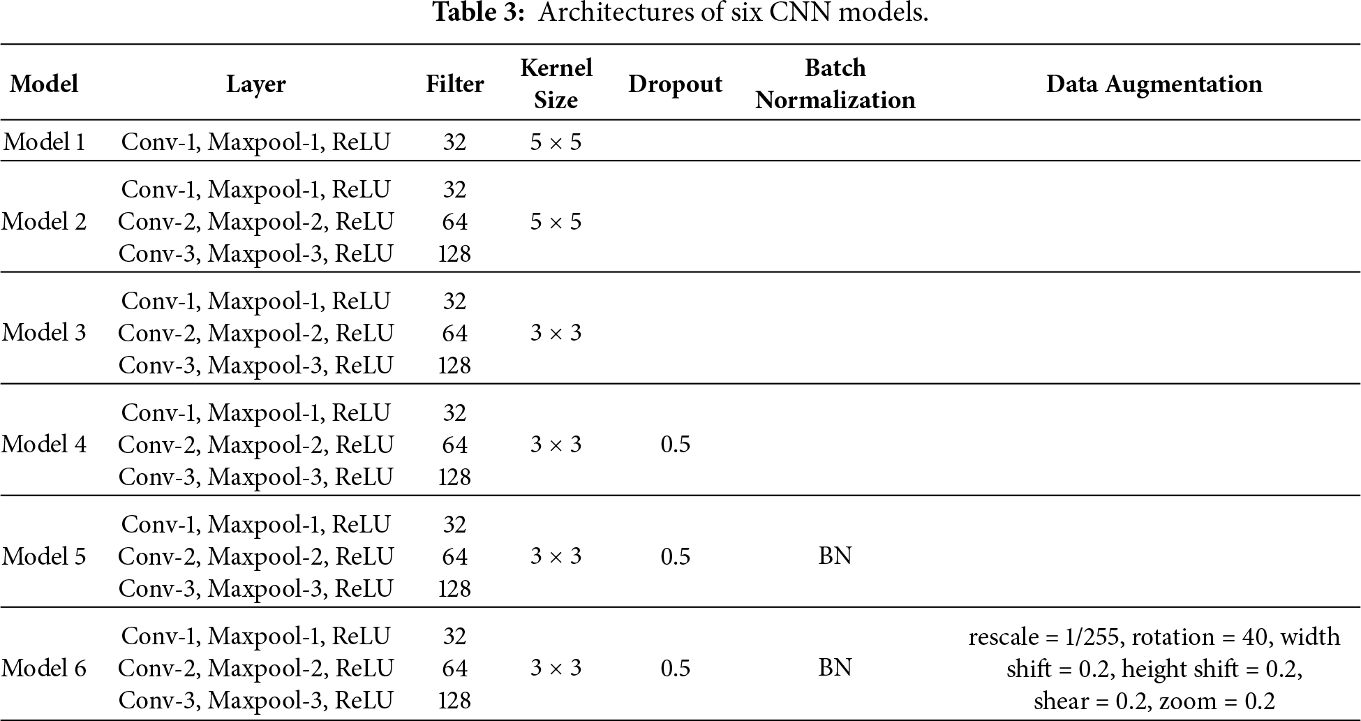
All CNN models incorporated convolutional, pooling, and fully connected layers (i.e., flatten, hidden, and output layers, respectively). A ReLU activation function was applied to the output of all the convolutional and fully connected layers, and a softmax function was used in the output layer. Model 1 had one convolution and one pooling layer, 32 filters, and a kernel size of 5 × 5; the two hidden layers contained 500 and 1000 neurons, respectively. Compared with shallow learning techniques, CNNs are constructed using deep network architecture and have more powerful feature representation capabilities, which make them more suitable for target detection. To this end, Model 2 was constructed with three convolutional layers, three pooling layers, and three fully connected layers. The number of filters in these layers was 32, 64, and 128, respectively, and the remaining parameters were the same as those in Model 1. In Model 3, the size of all the filters was changed from 5 × 5 to 3 × 3 on the basis of the original architecture of Model 2.

The kernel sizes of 3 × 3 and 5 × 5 were selected to capture image features at different spatial scales. The 3 × 3 kernels are effective for extracting fine-grained local patterns and have been widely adopted in deep CNN architectures due to their computational efficiency. In contrast, 5 × 5 kernels provide a larger receptive field, enabling the capture of more contextual and structural information. Evaluating both configurations allows an assessment of the impact of receptive field size on LULC classification performance.

Overfitting occurs when a learning network effectively classifies the training set but fails to provide satisfactory results for the validation and testing sets. The dropout method can be used to minimize overfitting in fully connected layers, reduce the complexity of the neural network connections, accelerate model training, and improve the generalizability of neural networks. In Model 4, a dropout of 0.5 was incorporated into the original architecture of Model 3. In Model 5, BN was used to reduce the number of convergences and achieve higher performance. Because the training data were limited, Model 6 was used to create more training images through data augmentation.

To quantify overfitting, an overfitting measure was defined as the difference between training and test accuracies. Specifically, the overfitting is calculated as the absolute difference between the final training accuracy and the corresponding test accuracy, normalized by 100: Overfitting = (|Acc_train − Acc_test|)/100. A higher overfitting value indicates greater overfitting and reduced generalization to unseen data. This accuracy-based metric provides an intuitive and practical means for comparing overfitting tendencies among different CNN configurations. All model hyperparameters were optimized through iterative experimentation, and the performance evaluation results for the six CNN models are summarized in Table 4.

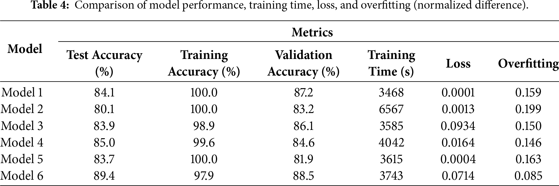
The training time reported in Table 4 corresponds to the total wall-clock time required to complete the full training process of each model, including 30 epochs, measured on a CPU-based system. All experiments were conducted on the same hardware platform (Intel Core TM i7 CPU with 32 GB RAM) using Python 3.8 and TensorFlow 2.9. The batch size and number of epochs were fixed at 32 and 30, respectively, for all models. Training time was measured at the model level rather than per image or per batch, and includes forward and backward propagation but excludes data loading and preprocessing overhead. Each model was trained once under identical conditions to enable fair comparison of computational efficiency across different CNN architectures.

When the kernel size is large (5 × 5), shallower convolutional and pooling layers are generally preferred; conversely, smaller kernels (3 × 3) are typically paired with deeper architectures. Moreover, larger kernels require longer training time due to increased computational cost. Compared with 3 × 3 kernels, 5 × 5 kernels significantly increase computational complexity, particularly under CPU-based training. In this study, models using 5 × 5 kernels required approximately twice the training time of those using 3 × 3 kernels. In Model 3, the kernel size was reduced from 5 × 5 to 3 × 3, resulting in higher test accuracy (83.9% versus 80.1% in Model 2) and reduced overfitting (approximately 4.9% lower than that of Model 2). This observation highlights the trade-off between receptive field size and computational efficiency and further supports the adoption of smaller convolutional kernels in subsequent models.

Overfitting still occurred when a dropout of 0.5 was incorporated into the hidden layer in Model 4. If dropout and data augmentation are used simultaneously, overfitting can be minimized. Reducing the number of neurons in a hidden layer by 1000 can reduce the accuracy on the testing set by approximately 10%. In Model 5, the convergence speed decreased when BN was performed. Using data augmentation and BN simultaneously can improve the overall performance of a detection model; the accuracy of Model 6 was 89.4%, and the overfitting was half that of all the other models in the experiment. The accuracy of the model that employed only data augmentation without BN was approximately 20% lower than that of Model 6.

Based on the results shown in Fig. 3, the training loss of Model 1 decreases rapidly and approaches zero, indicating strong fitting capability on the training data. However, its validation loss exhibits pronounced fluctuations, ranging from 0.29 to 3.05, suggesting limited stability in generalization performance. Model 2 demonstrates moderate overall performance, with both training and validation losses showing some fluctuations across epochs but remaining generally controllable. The training loss of Model 3 converges steadily; however, its validation loss fluctuates to a greater extent, with the final training and validation losses reaching 0.09 and 0.64, respectively. For Model 4, a relatively large gap is observed between the training and validation losses (0.016 and 0.96, respectively), indicating suboptimal generalization capability. In contrast, Model 5 achieves extremely low training loss, while its validation loss remains consistently high and unstable (approximately 0.66–2.23), revealing a clear tendency toward overfitting. As for Model 6, its training loss decreases steadily and converges during training. Although the validation loss exhibits an abnormal peak in the early epochs (up to 3.01), it gradually decreases as training progresses and reaches the lowest validation loss among all models (0.4007) at epoch 23, indicating superior generalization potential in the later training stage.

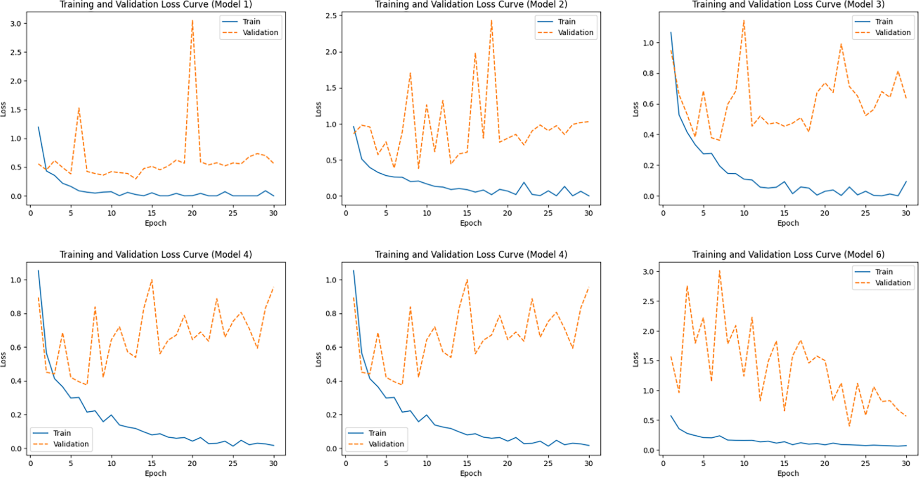
Figure 3: Training and validation loss curves for the six models.

Training a CNN follows the general paradigm of supervised learning, in which model parameters are iteratively updated using labeled samples to minimize the discrepancy between predicted and ground-truth classes. As shown by the learning curves, all six models exhibit a clear convergence trend over 30 epochs. Specifically, the training loss decreases sharply during the early epochs and then gradually stabilizes, indicating effective optimization (Fig. 4). For example, Model 5 converges rapidly, with the training loss dropping to approximately 0.012 by the eighth epoch and further decreasing to about 0.003 at the 30th epoch. The accuracy curves show a consistent increase in the training set across all configurations (Fig. 5). Training accuracy exceeds 0.90 within the first eight epochs and approaches approximately 0.97–1.00 by the end of training, indicating that the models fit the training data well. However, validation and testing accuracies remain consistently lower (generally below 0.90), leading to a clear performance gap between training and unseen data that suggests overfitting. In contrast, among the evaluated models, Model 6 exhibits the smallest gap and the most stable learning behavior, achieving the highest testing accuracy of 89.4%.

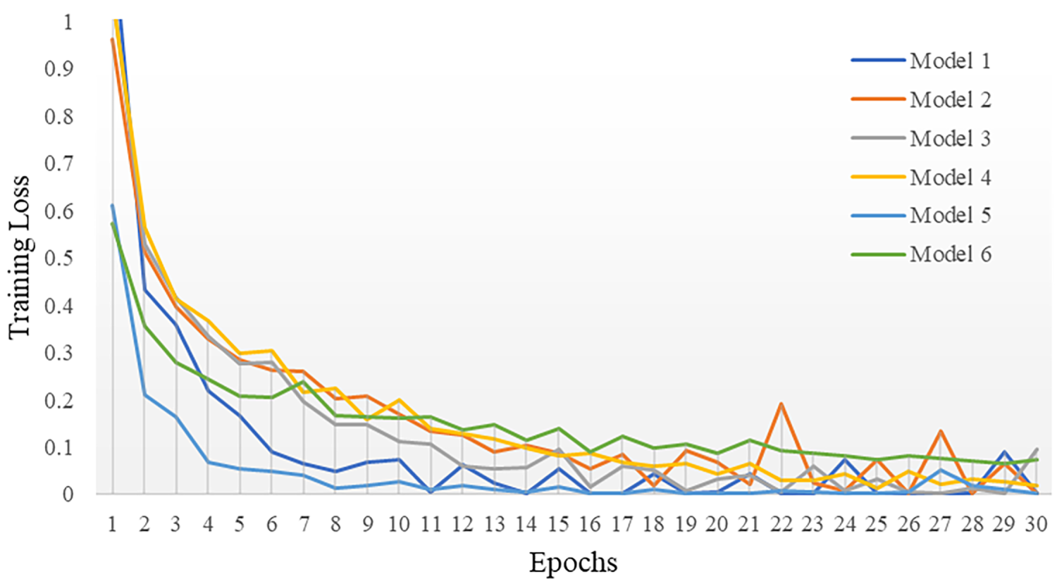
Figure 4: Loss of CNN models on training set.

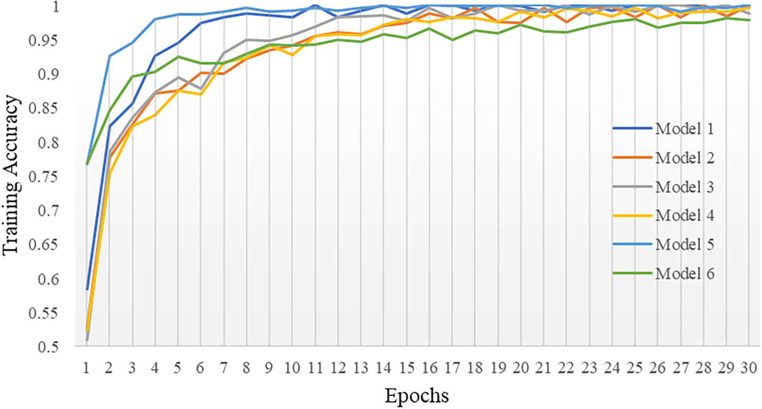
Figure 5: Accuracy of CNN models on training set.

To improve the clarity of the proposed architecture, an end-to-end pipeline diagram of Model 6 is presented in Fig. 6. The diagram illustrates the complete processing workflow, including the input patch size, the sequential convolutional modules, the corresponding tensor dimensions, and the final output definitions. Specifically, each UAV image patch of size 150 × 150 × 3 is progressively transformed through a series of convolutional and pooling operations, yielding hierarchical feature maps with decreasing spatial resolution and increasing channel depth. After feature flattening, the extracted representations are passed to the fully connected classification head, which produces predictions for four LULC classes via a softmax layer.

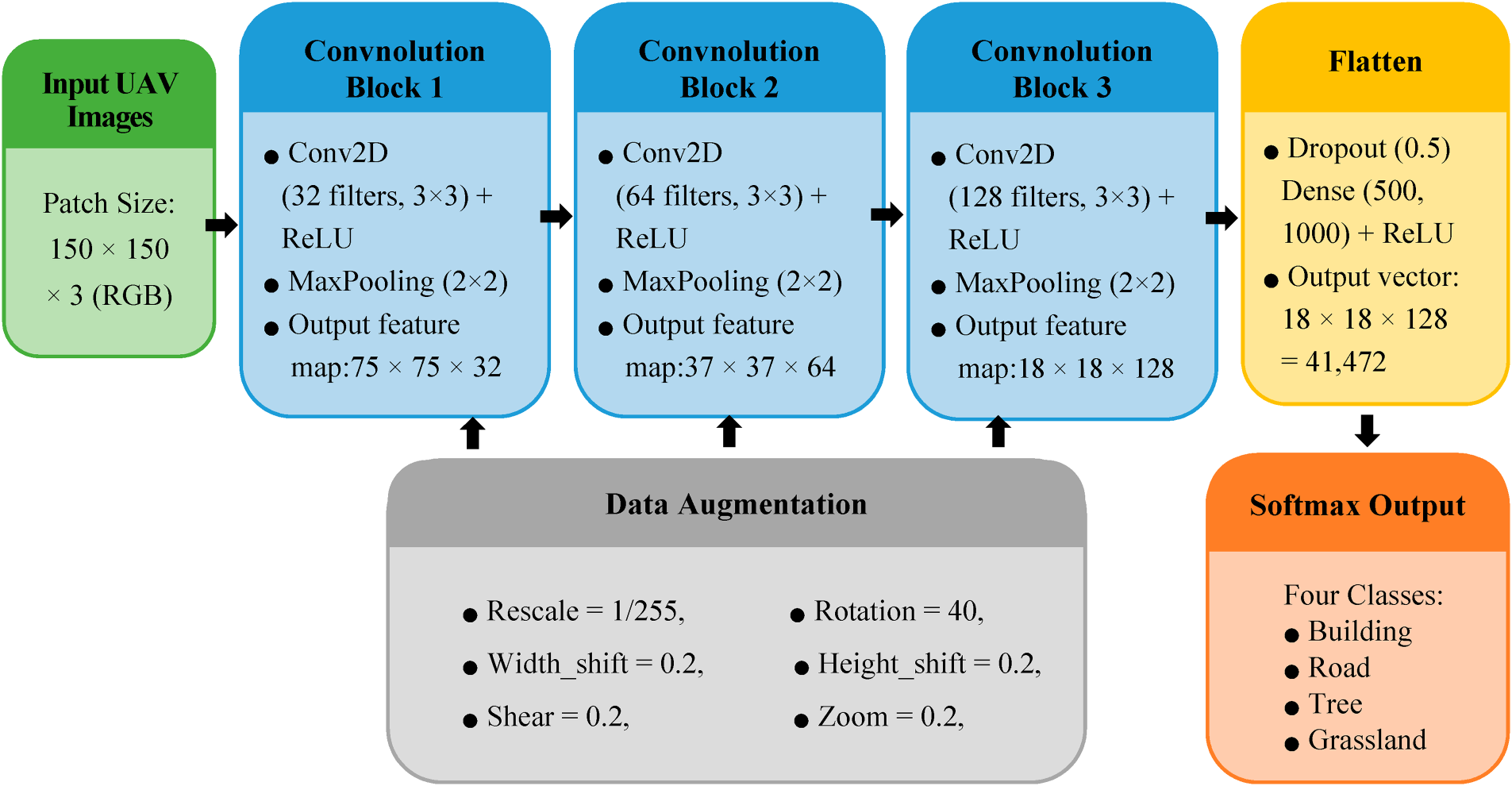
Figure 6: End-to-end pipeline of Model 6: from input patches to softmax-based classification.

In this study, development and optimization, including variations in the number of convolutional layers, filter sizes, dropout rates, and the use of batch normalization, were primarily guided by empirical experimentation rather than derived from formal theoretical analysis. This decision reflects the practical reality that, in deep learning applications involving high-resolution remote sensing imagery, model performance is often highly data-dependent and sensitive to contextual factors such as spatial texture, object scale, and class separability. Therefore, a trial-and-error approach was adopted to iteratively refine network configurations based on observed classification accuracy, overfitting behavior, and convergence patterns. This empirical methodology is consistent with prevailing practices in applied computer vision research.

3.2 Performance Evaluation of the Optimal Model

As illustrated in the graph in Fig. 7, the loss rates of Model 6 in detecting the four types of LULC in the training and validation image sets were similar. Most of the loss curves corresponding to training and validation sets follow consistent trends, but the loss curve corresponding to the detection of roads in the validation set fluctuates greatly. Roads close to buildings are often obscured by shadows, which may cause errors. Additionally, the sample contained more batches of building images than images of the other three land-use types, which may be attributed to the wide variability in building shapes and sizes observed in the images.

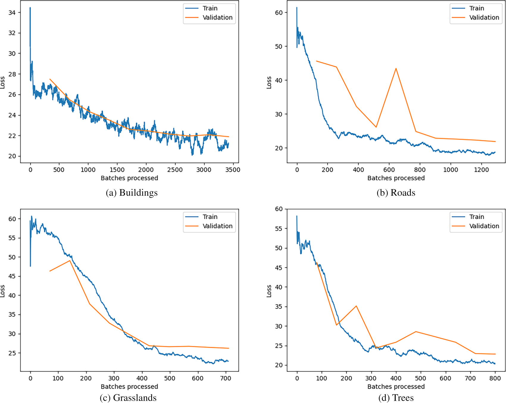
Figure 7: Loss of Model 6 in detecting four types of LULC.

This study evaluates the performance of Model 6 in classifying four land cover categories (Building, Road, Tree, and Grassland) using a confusion matrix as the primary analytical tool. According to the results of the confusion matrix, the model correctly classified 178 out of 200 images, achieving an overall accuracy of 89% (Fig. 8). Further analysis of the classification performance for each category indicates that the Grassland category achieved the highest recall at 94%, while the Tree category demonstrated the best F1 score at 91.8%, highlighting the model’s strong classification capabilities in these categories. However, notable misclassification issues were observed between the Building and Road categories, with 7 Road images misclassified as Building and 4 Building images misclassified as Road. This may be attributed to the spectral similarity between these two land cover types, indicating limitations in the model’s ability to extract features and differentiate subtle differences. Particularly when rooftops and adjacent paved surfaces exhibit similar grayscale tones and geometric patterns.

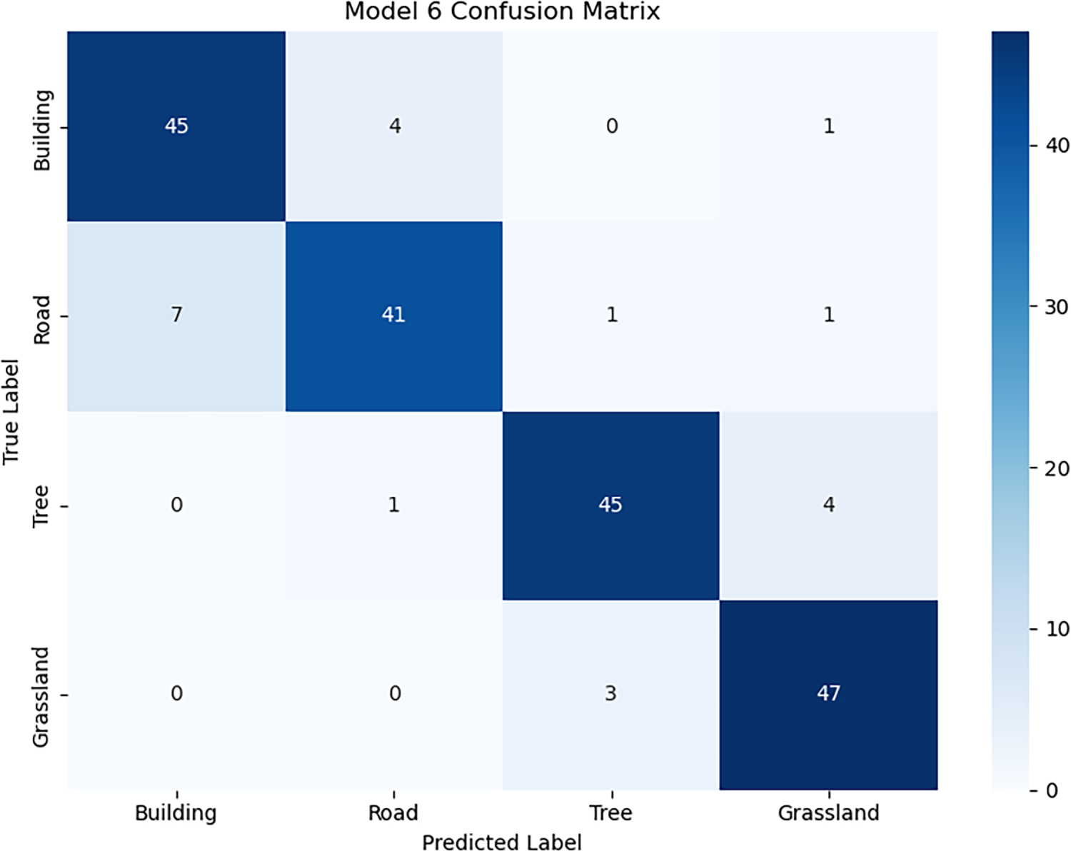
Figure 8: Classification results of Model 6 for four LULC.

The error distribution plot (Fig. 9) shows that Road has the highest number of false negatives, indicating that Road are most frequently missed or misclassified as other classes. Building and Tree show moderate but comparable levels of both false negatives and false positives, suggesting a relatively balanced, misclassification. Grassland has the fewest false negatives but a higher rate of false positives, suggesting that other classes are sometimes incorrectly assigned to Grassland. Together with the confusion matrix, this plot highlights that most errors are concentrated between spectrally or spatially similar classes (e.g., Road vs. Building and Tree vs. Grassland).

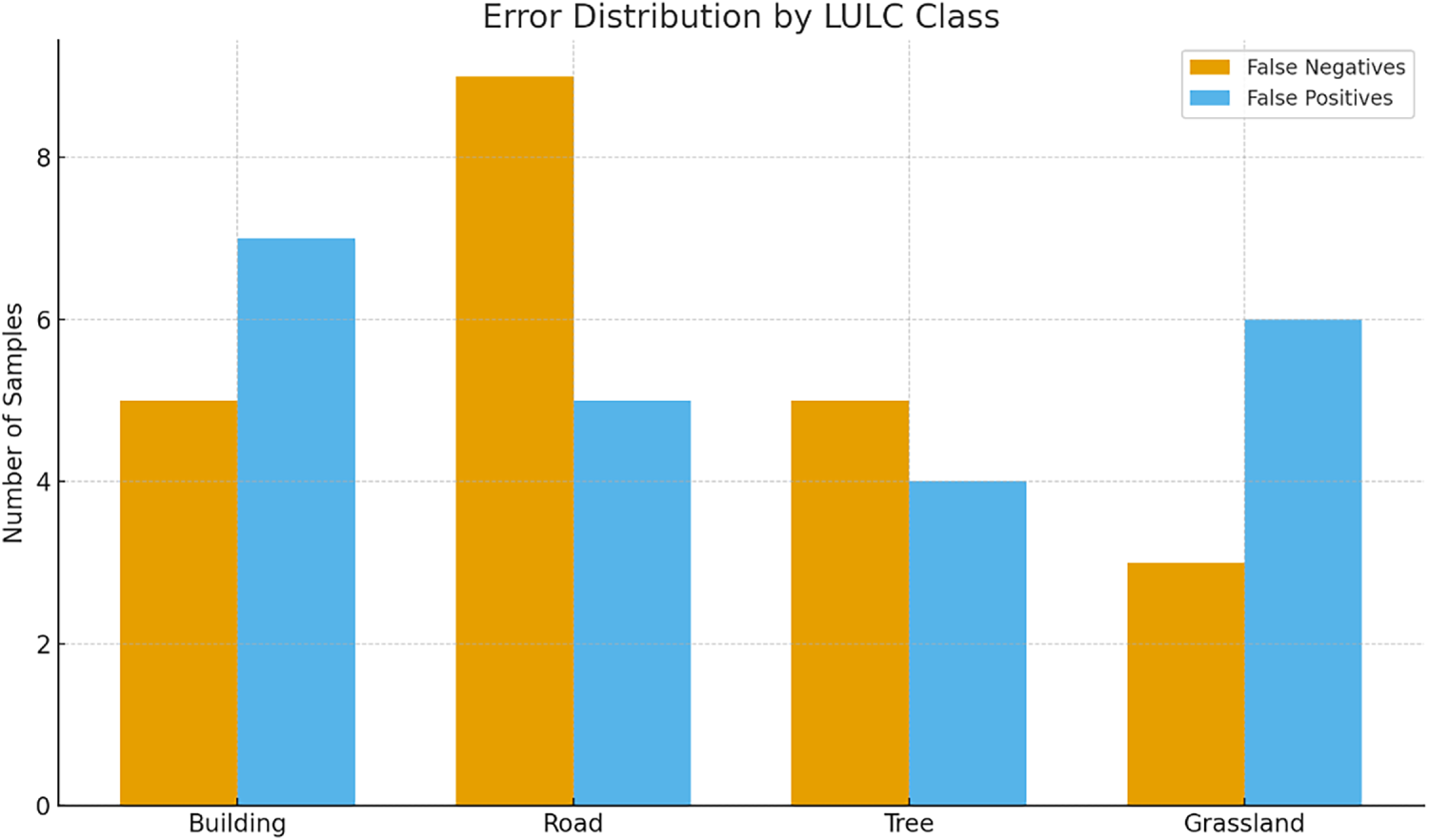
Figure 9: Error distribution of Model 6 across the four LULC classes.

Fig. 10 presents a Uniform Manifold Approximation and Projection (UMAP) cluster visualization of the feature embeddings generated by the Model 6 for the four LULC classes. The dimensionality reduction results reveal clear class-specific clusters, indicating that the model successfully learned discriminative latent representations. Building and Road features exhibit moderate spatial proximity, reflecting similarities in man-made surface patterns. In contrast, Tree and Grassland clusters are positioned farther apart, consistent with their distinct vegetative textures and spectral responses. Minimal overlap among clusters suggests strong inter-class separability and highlights the model’s ability to differentiate both artificial and natural surface types. The compactness of the Tree and Grassland clusters further implies stable within-class consistency, while the slightly elongated distribution of Road features reflects the heterogeneous appearance of road networks.

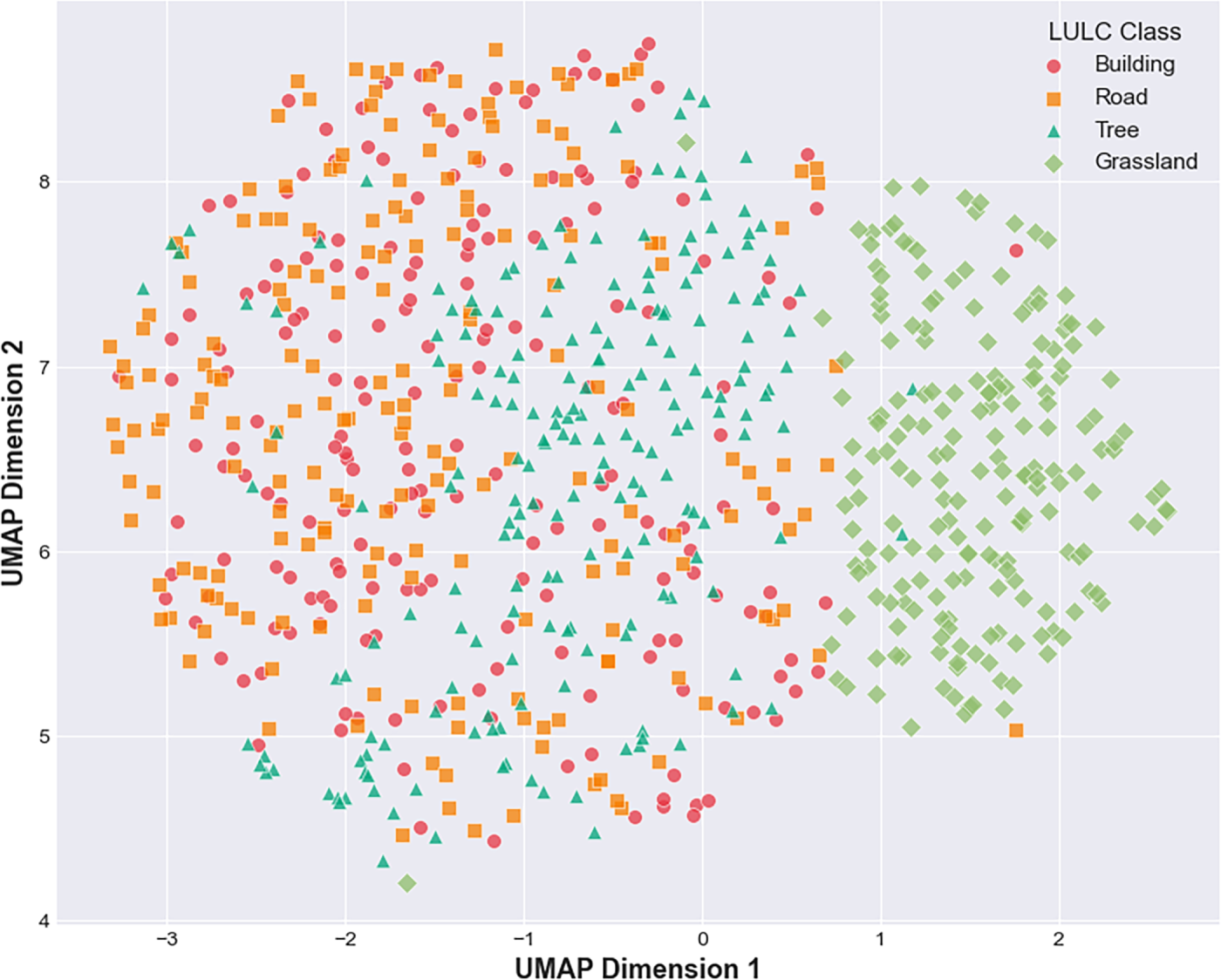
Figure 10: UMAP cluster visualization of LULC feature embeddings.

3.3 Model Evaluation Based on Confidence

In this study, the confidence score is the model’s predicted probability for the assigned class label, directly derived from the classifier’s final softmax layer. For each detected object i, the model produces a logit vector zi = [zi,1, zi,2, zi,3, zi,4] corresponding to the four classes: Building, Road, Tree, and Grassland. The softmax function transforms these logits into normalized probabilities as:

Pi,c=−ezi,c∑k=14ezi,k(5)

where Pi,c is the probability that object i belongs to category c. The confidence for each object is then defined as the maximum predicted probability among the four classes:

Confidencei=max(Pi,1,Pi,2,Pi,3,Pi,4)(6)

Thus, the confidence value ranges from 0 to 1, where values closer to 1 indicate greater model certainty in its classification.

The confidence-based evaluation provides additional insight into the Model 6 prediction reliability across the four LULC classes. Fig. 11 indicates that Tree and Grassland exhibit the highest confidence stability, with narrow interquartile ranges and medians above 0.90, reflecting consistently strong agreement between predicted and actual labels. The building shows moderate variability, suggesting occasional spectral or textural ambiguity in the input imagery. In contrast, Road shows the widest spread and a lower median confidence, consistent with its comparatively lower recall and the greater intra-class heterogeneity typically observed in linear ground features. Overall, the distribution patterns corroborate the model’s quantitative metrics, indicating robust classification performance while highlighting class-specific uncertainty.

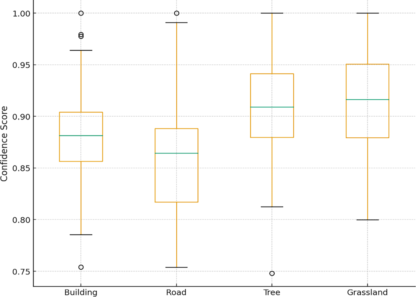
Figure 11: Grouped boxplot of confidence score distributions for the four LULC classes.

The grouped histograms in Fig. 12 illustrate the confidence score distributions across the four LULC classes, offering insights into the classifier’s reliability and error structure. Building and Grassland exhibit highly concentrated high-confidence predictions, reflecting strong model separability and consistent feature representation. Tree also demonstrates a narrow, right-skewed distribution, indicating robust discrimination despite moderate class variability. In contrast, Road displays a more dispersed distribution with a noticeable tail toward lower confidence values, aligning with its comparatively lower recall and suggesting higher intra-class heterogeneity or spectral confusion with adjacent categories. The clear separation between correct and incorrect prediction distributions further supports the model’s stability, while the overlap observed in the Road class highlights areas requiring enhanced feature extraction or additional contextual information.

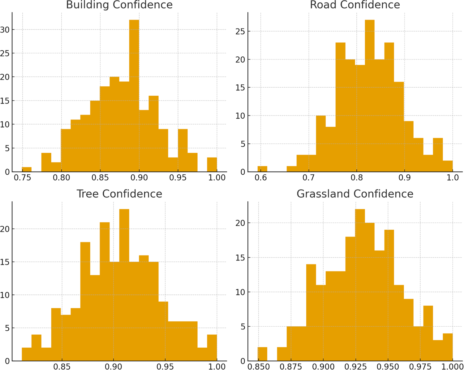
Figure 12: Grouped histograms of confidence score distributions for the four LULC classes.

The kernel density estimation (KDE) curves illustrate the distributions of confidence scores for the four LULC classes and provide insights into the Model 6 probabilistic behavior (Fig. 13). Tree and Grassland exhibit sharply peaked densities centered around 0.92–0.95, indicating highly consistent predictions with minimal dispersion. Building shows a moderately concentrated density around 0.90, reflecting stable yet slightly more variable confidence outputs. In contrast, Road displays a broader, left-shifted distribution, with the-density mass extending toward lower confidence values near 0.80, suggesting greater uncertainty in distinguishing road features from visually similar classes. Overall, the KDE profiles reveal a clear separation among classes, with vegetation-related categories achieving the highest prediction certainty, while man-made surfaces exhibit relatively higher intra-class variability.

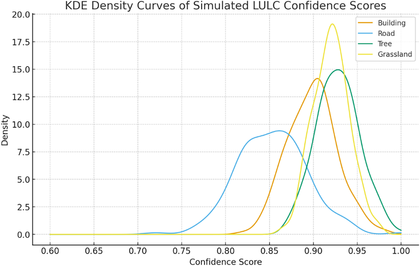
Figure 13: KDE curves of simulated confidence score distributions for four LULC classes.

4  Discussion

4.1 Comparison with Baseline CNN Models

To further contextualize the performance of Model 6 from an architectural perspective, three representative CNN backbones, ResNet, EfficientNet, and MobileNet, were considered for comparative analysis. All models were intentionally trained from scratch to enable a controlled analysis of CNN architectural configurations and hyperparameter effects under identical conditions, without introducing external pretrained knowledge. This design choice ensures that observed performance differences can be attributed to internal model design rather than prior information learned from large-scale natural image datasets such as ImageNet. While transfer learning is widely adopted in small-data scenarios and often improves performance, it may also introduce domain bias when pretrained on datasets with significantly different visual characteristics. Given the study’s primary objective of examining architecture-level effects in UAV-based LULC classification, transfer learning was not included in the current experimental scope.

As summarized in Table 5, the per-class evaluation results for Model 6 indicate robust and well-balanced classification performance. Specifically, the building class achieves a precision, recall, and F1-score of 0.87, 0.90, and 0.88, respectively, demonstrating effective identification of building instances while maintaining reliable accuracy. The road class attains a precision of 0.89 and a recall of 0.82, resulting in a slightly lower F1-score of 0.85, which may be attributed to the elongated geometry of roads in UAV imagery and their frequent confusion with surrounding land cover types. For natural land cover categories, the tree class records a precision of 0.92, a recall of 0.90, and an F1-score of 0.91, while the grassland class achieves corresponding values of 0.89, 0.94, and 0.91. These results indicate that Model 6 exhibits stable and consistent performance across natural land cover types. Overall, all four classes achieve F1-scores above 0.85 in Model 6, reflecting a well-balanced classification capability.

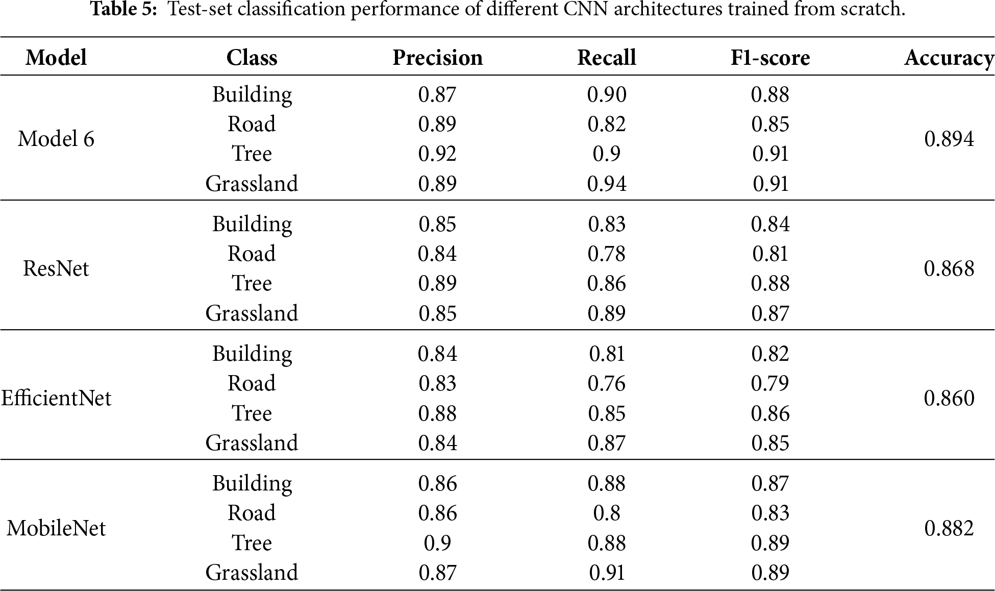
In contrast, the baseline CNN architectures trained from scratch show relatively lower and less consistent test-set performance across classes. ResNet and EfficientNet achieve lower overall accuracies (0.868 and 0.860, respectively), with noticeably reduced recall and F1-scores for the road class, suggesting limited generalization under small-sample conditions. MobileNet attains a higher overall accuracy (0.882) and more balanced per-class F1-scores compared with the deeper architectures, indicating that lightweight models may generalize more stably when training data are limited. Nevertheless, its performance remains slightly inferior to that of Model 6, highlighting the effectiveness of the proposed architecture in balancing model complexity and classification performance under from-scratch training conditions.

It should be noted that all experiments in this study were conducted within a single geographic region under consistent image acquisition conditions, including the same UAV platform and a limited time window. While this controlled setting reduces confounding factors and facilitates a focused architectural analysis, it also defines a clear applicability boundary for the reported results. When applied across different geographic areas or seasonal conditions, variations in land-cover appearance, illumination, vegetation phenology, and background context may degrade classification performance. Addressing such cross-region and cross-season generalization remains an important topic for future work and may benefit from larger multi-region datasets. Despite this limitation, the controlled experimental setting allows a clearer assessment of architectural design choices under consistent conditions.

In addition to classification accuracy, computational efficiency is a critical consideration for UAV-based LULC applications, where onboard or edge deployment often imposes strict constraints on memory footprint and inference speed. To account for stochastic variability arising from random initialization and training dynamics, experiments were repeated with five different random seeds under an identical train/validation/test split; results are reported as mean ± standard deviation. Table 6 summarizes both predictive performance and computational cost for Model 6 and the baseline CNN architectures, including parameter count, floating-point operations (FLOPs), Macro-F1, and inference latency, all measured on the same hardware platform.

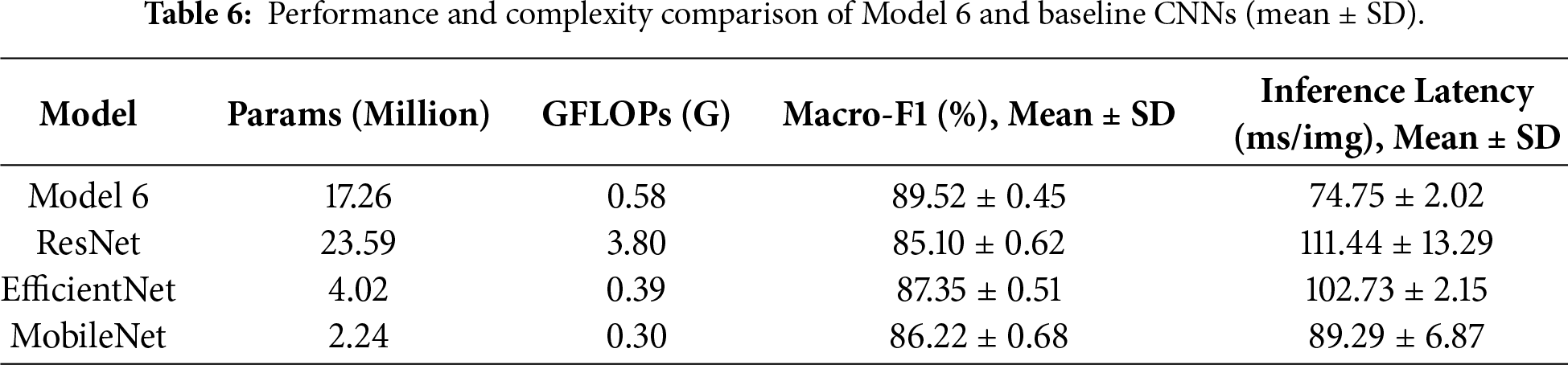
Model 6 comprises 17.26 million parameters and requires 0.58 GFLOPs, achieving the highest Macro-F1 of 89.52% ± 0.45 with the lowest average inference latency of 74.75 ± 2.02 ms per image. In comparison, ResNet exhibits substantially higher computational complexity (3.80 GFLOPs) and a significantly longer latency of 111.44 ± 13.29 ms, while yielding the lowest classification performance. Although EfficientNet and MobileNet feature fewer parameters and lower theoretical FLOPs, their practical inference latencies on the CPU platform (102.73 and 89.29 ms, respectively) are higher than that of Model 6. Furthermore, their Macro-F1 scores remain inferior to those of Model 6, particularly under limited training data conditions. Overall, Model 6 achieves a superior balance between efficiency and performance. Notably, it outperforms all baselines in both classification accuracy and actual inference speed on the target hardware, despite not being the smallest in parameter count. This confirms Model 6 as a highly optimized and practically deployable architecture for UAV-based LULC tasks.

In addition, CNN-based frameworks applied to UAV images commonly achieve overall classification accuracies in the range of 85%–95%, depending on factors such as data modality and scene complexity. For instance, in UAV-based LULC classification using ResNet50 and DenseNet121 architectures, accuracies around 92% have been reported [30]. In a hybrid Transformer-CNN approach (DE-UNet), performance surpassed that of UNet and UNet++ by approximately 0.3%–4.8% [31]. Lightweight CNNs, such as MV2-CBAM, have also yielded mean accuracies of approximately 86%–88% [32]. Rajkumar et al. [33] applied eight pre-trained scene-level CNN models (e.g., VGG19, ResNet152V2, EfficientNetB5, DenseNet201) and achieved an accuracy of over 97% on multispectral UAV forest imagery, demonstrating the gains possible when using larger models and richer spectral bands.

To reduce the misclassification between the Building and Road classes in Model 6 and to further improve classification accuracy, an additional validation experiment was conducted. While keeping the Model 6 architecture and all training hyperparameters unchanged (including the optimizer, learning rate, batch size, and number of epochs), only the data augmentation strategy was modified by incorporating illumination and shadow augmentation. This adjustment was intended to enhance the model’s robustness to varying illumination conditions and shadow occlusions commonly observed in UAV imagery. Specifically, a customized preprocessing function (preprocess_with_illum_shadow) was integrated into the data augmentation pipeline, introducing random brightness and contrast adjustments, gamma correction, and synthetic shadow masks to simulate illumination variability and cast-shadow effects.

As shown in the updated confusion matrix in Fig. 14, the mutual misclassification between Building and Road classes is noticeably reduced. The number of Building samples misclassified as Road decreased from 4 to 2 (a reduction of 50%), while the number of Road samples misclassified as Building decreased from 7 to 4 (a reduction of 42.9%). These results indicate that illumination and shadow augmentation effectively mitigate confusion caused by shadow coverage, material reflectance variations, and similar linear structural patterns between these two man-made land cover types. In terms of class-wise performance, the recall for the Building class increased to 94%, and the recall for the Road class improved to 88%, reflecting enhanced recognition stability for man-made surfaces. Notably, the numbers of correctly classified Tree and Grassland samples remained unchanged (45 and 47, respectively), suggesting that the proposed augmentation strategy primarily improves discrimination between man-made classes without introducing adverse effects on natural land cover recognition.

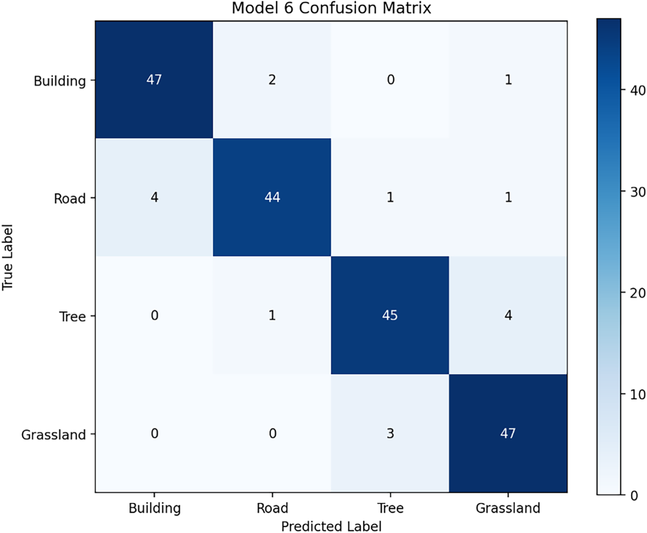
Figure 14: Confusion matrix of Model 6 with illumination and shadow augmentation.

4.2 Applications and Limitations

The proposed framework targets scene-level LULC classification rather than pixel-wise map generation. Each UAV image tile is treated as an independent scene and assigned a dominant LULC label, enabling rapid land cover identification and region-level analysis. Compared with semantic segmentation approaches that produce dense pixel-level maps but require extensive annotations and higher computational cost, the adopted patch-based classification strategy provides a lightweight and data-efficient alternative. This design is well suited for high-resolution UAV applications that support timely decision-making in urban planning, environmental monitoring, and resource management.

Although the proposed method demonstrates satisfactory performance in several aspects, certain limitations remain and are discussed below.

(1)   The dataset utilized in this study comprises 800 manually labeled UAV image samples, which, while sufficient for initial model development and controlled evaluation, may not be adequate to ensure generalizability across broader geographic regions and varying environmental conditions. As all images were collected from a single study area, the model’s exposure to diverse land cover types, climatic variability, and seasonal dynamics is inherently limited [34]. Consequently, the findings should be interpreted as location-specific and scenario-dependent rather than universally representative.

(2)   Despite Model 6 incorporating dropout, batch normalization, and data augmentation, a noticeable gap remains between training and testing performance, with training accuracy (97.9%) substantially exceeding the testing accuracy (89.4%). This discrepancy indicates persistent overfitting and suggests that the learned representations may partially capture dataset-specific patterns rather than fully generalizable features, which is plausible given the relatively limited dataset size. Although the adopted regularization strategies improved training stability and robustness, further gains in generalization may be achieved by reducing model capacity. In addition, applying weight decay (L2 regularization) could further penalize overly complex parameter values and help control model complexity, thereby improving generalization performance. These strategies were not explored in the current study in order to maintain controlled comparisons among the evaluated configurations, but they represent promising directions for future work.

(3)   Although all models in this study were trained from scratch to ensure a controlled architectural comparison, future work may investigate transfer-learning-based approaches, which have the potential to improve performance in small-data UAV scenarios further.

(4)   In this study, four LULC categories, buildings, roads, trees, and grasslands, were selected based on their prevalence and relevance to the urban landscape of the study area. These classes sufficiently meet the classification requirements for this specific geographic context and application scope. While the inclusion of only four categories limits the model’s direct applicability to more complex or heterogeneous environments, the current configuration serves as a necessary baseline for evaluating model performance under controlled conditions. Encompassing additional LULC classes and more diverse landscapes thereby enhances the model’s generalizability and utility in broader real-world scenarios [35].

(5)   A fully spatially independent split (e.g., block-based or region-wise partitioning) would provide a more rigorous assessment of spatial generalization. However, given the limited spatial extent of the study area and the relatively small dataset size, such a split would substantially reduce the number of training samples and hinder stable model optimization. This limitation is acknowledged, and future work will explore spatially independent evaluation strategies using larger, multi-region UAV datasets.

(6)   Although the RMSprop optimizer facilitates stable optimization, the training process becomes more time-consuming when larger convolutional kernels are used. Given that this study used CPU-based computation, these computational constraints may limit the feasibility of real-time deployment [36]. Future work may address this issue by incorporating GPU acceleration.

The experimental design aligns directly with the contributions outlined in the Introduction, with each experimental group serving a distinct role. Initially, Models 1–5 are used to conduct an ablation study examining the impact of individual architectural components and training strategies on performance. Subsequently, Model 6 represents the culmination of these findings, combining the identified effective elements into a robust CNN architecture optimized for LULC tasks. To establish practical relevance, the proposed model is further evaluated against widely adopted baseline architectures, including ResNet, EfficientNet, and MobileNet, in terms of both performance and computational efficiency. Collectively, these experimental groups provide complementary evidence supporting the claimed contributions and demonstrate the methodological soundness and practical applicability of the proposed approach.

5  Conclusion

With the continuous development of UAV remote sensing technology, high-resolution images will become more commonplace, and image data will become more affordable, convenient, and easier to acquire. Although UAVs can be used to acquire high-resolution images with detailed textural information, traditional pixel- and object-based classification methods cannot effectively distinguish such details, which can result in misclassification. Therefore, a CNN-based deep learning method for image recognition is proposed to distinguish small objects in high-resolution images based on their shapes, textures, and other fine details, thereby facilitating the detection and classification of LULC in UAV images.

This study systematically examined the effects of different CNN architectures and hyperparameter settings on UAV-based LULC classification performance. The results demonstrate that kernel size plays a critical role in feature extraction, with smaller 3 × 3 kernels providing improved representation of fine-grained spatial patterns compared to larger 5 × 5 kernels. The inclusion of dropout and batch normalization further enhanced model generalization by mitigating overfitting and stabilizing the training process. In addition, data augmentation significantly improved robustness to spatial variability and contributed to more consistent validation performance.

Parameter adjustment plays a critical role in image classification, as it directly influences model generalization and the prevention of overfitting while enabling high detection accuracy. Among all evaluated configurations, Model 6 achieved the best overall performance by integrating a 3 × 3 convolutional kernel, dropout (0.5), batch normalization, and data augmentation (rescale = 1/255, rotation = 40, width shift = 0.2, height shift = 0.2, shear = 0.2, and zoom = 0.2), while maintaining a fixed optimizer (RMSprop), learning rate, and batch size. This configuration effectively balances model complexity, generalization capability, and computational efficiency, thereby fulfilling the study’s objective of identifying an optimized CNN architecture for high-resolution UAV-based LULC classification. Model 6 achieved the highest detection performance across all LULC classes, with an overall accuracy of 89.4% and a loss value of 0.0714. Although the remaining five models also attained accuracies above 80.0% and loss values below 0.09, they exhibited more pronounced overfitting behavior compared with Model 6.

As UAVs become cheaper and easier to acquire, the acquisition of UAV images will become more efficient. Integrating high-resolution images with deep learning methods can benefit monitoring and surveying operations, such as the detection of collapsed buildings after earthquakes, road damage, illegal rooftop structures, and crop yields. In the future, researchers should continue optimizing deep neural networks of LULC detection and classification.

Acknowledgement: The author gratefully acknowledges the use of ChatGPT-5 and Grammarly Pro (v1.2.224.1806) for linguistic refinement. During the preparation of this work, these tools were employed to enhance readability. After their use, the author thoroughly reviewed and revised the content to ensure scientific accuracy and takes full responsibility for the final version of the publication. The author also wishes to express sincere appreciation to Dr. Yu-Jen Chung of the Department of Marine Science, ROC Naval Academy, for generously providing access to a UAV, which greatly facilitated the efficient collection of the deep learning dataset used for land use and land cover classification.

Funding Statement: The author received no specific funding for this study.

Availability of Data and Materials: Data available on request from the authors.

Ethics Approval: Not applicable.

Conflicts of Interest: The author declares no conflicts of interest.

References

1. Masoumi Z, van Genderen J. Artificial intelligence for sustainable development of smart cities and urban land-use management. Geo Spatial Inf Sci. 2024;27(4):1212–36. doi:10.1080/10095020.2023.2184729. [Google Scholar] [CrossRef]

2. Lou C, Al-qaness MAA, AL-Alimi D, Dahou A, Abd Elaziz M, Abualigah L, et al. Land use/land cover (LULC) classification using hyperspectral images: a review. Geo Spatial Inf Sci. 2025;28(2):345–86. doi:10.1080/10095020.2024.2332638. [Google Scholar] [CrossRef]

3. Rhee DS, Do Kim Y, Kang B, Kim D. Applications of unmanned aerial vehicles in fluvial remote sensing: an overview of recent achievements. KSCE J Civ Eng. 2018;22(2):588–602. doi:10.1007/s12205-017-1862-5. [Google Scholar] [CrossRef]

4. Yao H, Qin R, Chen X. Unmanned aerial vehicle for remote sensing applications—a review. Remote Sens. 2019;11(12):1443. doi:10.3390/rs11121443. [Google Scholar] [CrossRef]

5. Mollick T, Azam MG, Karim S. Geospatial-based machine learning techniques for land use and land cover mapping using a high-resolution unmanned aerial vehicle image. Remote Sens Appl Soc Environ. 2023;29:100859. doi:10.1016/j.rsase.2022.100859. [Google Scholar] [CrossRef]

6. Hwangbo JW, Yu K. Decision support system for the selection of classification methods for remote sensing imagery. KSCE J Civ Eng. 2010;14(4):589–600. doi:10.1007/s12205-010-0589-3. [Google Scholar] [CrossRef]

7. Jensen JR, Qiu F, Patterson K. A neural network image interpretation system to extract rural and urban land use and land cover information from remote sensor data. Geocarto Int. 2001;16(1):21–30. doi:10.1080/10106040108542179. [Google Scholar] [CrossRef]

8. Yang H, Ma B, Du Q, Yang C. Improving urban land use and land cover classification from high-spatial-resolution hyperspectral imagery using contextual information. J Appl Remote Sens. 2010;4(1):041890. doi:10.1117/1.3491192. [Google Scholar] [CrossRef]

9. Vetrivel A, Gerke M, Kerle N, Vosselman G. Identification of damage in buildings based on gaps in 3D point clouds from very high resolution oblique airborne images. ISPRS J Photogramm Remote Sens. 2015;105(16):61–78. doi:10.1016/j.isprsjprs.2015.03.016. [Google Scholar] [CrossRef]

10. Huang B, Zhao B, Song Y. Urban land-use mapping using a deep convolutional neural network with high spatial resolution multispectral remote sensing imagery. Remote Sens Environ. 2018;214(3):73–86. doi:10.1016/j.rse.2018.04.050. [Google Scholar] [CrossRef]

11. Zhang L, Huang X, Huang B, Li P. A pixel shape index coupled with spectral information for classification of high spatial resolution remotely sensed imagery. IEEE Trans Geosci Remote Sensing. 2006;44(10):2950–61. doi:10.1109/tgrs.2006.876704. [Google Scholar] [CrossRef]

12. Verburg PH, Neumann K, Nol L. Challenges in using land use and land cover data for global change studies. Glob Change Biol. 2011;17(2):974–89. doi:10.1111/j.1365-2486.2010.02307.x. [Google Scholar] [CrossRef]

13. Zhao B, Zhong Y, Zhang L. A spectral-structural bag-of-features scene classifier for very high spatial resolution remote sensing imagery. ISPRS J Photogramm Remote Sens. 2016;116(3):73–85. doi:10.1016/j.isprsjprs.2016.03.004. [Google Scholar] [CrossRef]

14. Blaschke T. Object based image analysis for remote sensing. ISPRS J Photogramm Remote Sens. 2010;65(1):2–16. doi:10.1016/j.isprsjprs.2009.06.004. [Google Scholar] [CrossRef]

15. Maboudi M, Amini J, Malihi S, Hahn M. Integrating fuzzy object based image analysis and ant colony optimization for road extraction from remotely sensed images. ISPRS J Photogramm Remote Sens. 2018;138(2):151–63. doi:10.1016/j.isprsjprs.2017.11.014. [Google Scholar] [CrossRef]

16. Zhang C, Sargent I, Pan X, Li H, Gardiner A, Hare J, et al. Joint Deep Learning for land cover and land use classification. Remote Sens Environ. 2019;221:173–87. doi:10.1016/j.rse.2018.11.014. [Google Scholar] [CrossRef]

17. Ma L, Li M, Ma X, Cheng L, Du P, Liu Y. A review of supervised object-based land-cover image classification. ISPRS J Photogramm Remote Sens. 2017;130(142):277–93. doi:10.1016/j.isprsjprs.2017.06.001. [Google Scholar] [CrossRef]

18. Xia GS, Hu J, Hu F, Shi B, Bai X, Zhong Y, et al. AID: a benchmark data set for performance evaluation of aerial scene classification. IEEE Trans Geosci Remote Sens. 2017;55(7):3965–81. doi:10.1109/TGRS.2017.2685945. [Google Scholar] [CrossRef]

19. Mahendra HN, Pushpalatha V, Mallikarjunaswamy S, Rama Subramoniam S, Sunil Rao A, Sharmila N. LULC change detection analysis of Chamarajanagar district, Karnataka state, India using CNN-based deep learning method. Adv Space Res. 2024;74(12):6384–408. doi:10.1016/j.asr.2024.07.066. [Google Scholar] [CrossRef]

20. Anitha V, Kalaiselvi S, Gomathi V, Manimegalai D. A lightweight CNN for LULC classification: an alpha-cut fuzzy geometric normalization approach. Signal Image Video Process. 2025;19(9):753. doi:10.1007/s11760-025-04349-4. [Google Scholar] [CrossRef]

21. Yang B, Wang S, Zhou Y, Wang F, Hu Q, Chang Y, et al. Extraction of road blockage information for the Jiuzhaigou earthquake based on a convolution neural network and very-high-resolution satellite images. Earth Sci Inform. 2020;13(1):115–27. doi:10.1007/s12145-019-00413-z. [Google Scholar] [CrossRef]

22. Tan X, Xue Z. Spectral-spatial multi-layer perceptron network for hyperspectral image land cover classification. Eur J Remote Sens. 2022;55(1):409–19. doi:10.1080/22797254.2022.2087540. [Google Scholar] [CrossRef]

23. Hussain K, Mehmood K, Sun Y, Badshah T, Ahmad Anees S, Shahzad F, et al. Analysing LULC transformations using remote sensing data: insights from a multilayer perceptron neural network approach. Ann GIS. 2025;31(3):473–500. doi:10.1080/19475683.2024.2343399. [Google Scholar] [CrossRef]

24. Hadi SJ, Ahmed I, Iqbal A, Alzahrani AS. CATR: cNN augmented transformer for object detection in remote sensing imagery. Sci Rep. 2025;15(1):42281. doi:10.1038/s41598-025-27872-3. [Google Scholar] [PubMed] [CrossRef]

25. Sultan N, Ruangsang W, Aramvith S. HybridATNet: multi-scale attention and hybrid feature refinement network for remote sensing image super-resolution. IEEE Access. 2025;13:159979–97. doi:10.1109/ACCESS.2025.3608009. [Google Scholar] [CrossRef]

26. Sharma A, Liu X, Yang X, Shi D. A patch-based convolutional neural network for remote sensing image classification. Neural Netw. 2017;95(9):19–28. doi:10.1016/j.neunet.2017.07.017. [Google Scholar] [PubMed] [CrossRef]

27. Wang Y, Wang Z. A survey of recent work on fine-grained image classification techniques. J Vis Commun Image Represent. 2019;59(C):210–4. doi:10.1016/j.jvcir.2018.12.049. [Google Scholar] [CrossRef]

28. Al-Najjar HAH, Kalantar B, Pradhan B, Saeidi V, Halin AA, Ueda N, et al. Land cover classification from fused DSM and UAV images using convolutional neural networks. Remote Sens. 2019;11(12):1461. doi:10.3390/rs11121461. [Google Scholar] [CrossRef]

29. Bai Y, Mas E, Koshimura S. Towards operational satellite-based damage-mapping using U-Net convolutional network: a case study of 2011 tohoku earthquake-tsunami. Remote Sens. 2018;10(10):1626. doi:10.3390/rs10101626. [Google Scholar] [CrossRef]

30. Yaloveha V, Podorozhniak A, Kuchuk H, Garashchuk N. Performance comparison of CNNs on high-resolution multispectral dataset applied to land cover classification problem. Reks. 2023(2):107–18. doi:10.32620/reks.2023.2.09. [Google Scholar] [CrossRef]

31. Lu T, Wan L, Qi S, Gao M. Land cover classification of UAV remote sensing based on transformer-CNN hybrid architecture. Sensors. 2023;23(11):5288. doi:10.3390/s23115288. [Google Scholar] [PubMed] [CrossRef]

32. Deng X, Shi M, Khan B, Choo YH, Ghaffar F, Lim CP. A lightweight CNN model for UAV-based image classification. Soft Comput. 2025;29(4):2363–78. doi:10.1007/s00500-025-10512-3. [Google Scholar] [CrossRef]

33. Rajkumar M, Nagarajan S, DeWitt P. Land use land cover mapping using uas imagery: Scene classification and semantic segmentation. In: International Archives of the Photogrammetry, Remote Sensing and Spatial Information Sciences; 2022 Mar 21–25; Denver, Colorado, USA. p. 177–84. doi:10.5194/isprs-archives-xlvi-m-2-2022-177-2022. [Google Scholar] [CrossRef]

34. Rengma NS, Yadav M. Generation and classification of patch-based land use and land cover dataset in diverse Indian landscapes: a comparative study of machine learning and deep learning models. Environ Monit Assess. 2024;196(6):568. doi:10.1007/s10661-024-12719-7. [Google Scholar] [PubMed] [CrossRef]

35. Osco LP, Marcato J Jr, Marques Ramos AP, de Castro Jorge LA, Fatholahi SN, de Andrade Silva J, et al. A review on deep learning in UAV remote sensing. Int J Appl Earth Obs Geoinf. 2021;102:102456. doi:10.1016/j.jag.2021.102456. [Google Scholar] [CrossRef]

36. Pashaei M, Kamangir H, Starek MJ, Tissot P. Review and evaluation of deep learning architectures for efficient land cover mapping with UAS hyper-spatial imagery: a case study over a wetland. Remote Sens. 2020;12(6):959. doi:10.3390/rs12060959. [Google Scholar] [CrossRef]