Multi-Granularity Traffic Prediction for Satellite Networks Based on Dynamic Adaptive Graph Modeling

1  Introduction

Due to the advantages of global coverage and random access, the satellite network has gained more and more attention in recent years [1,2]. While the traditional terrestrial networks can offer stable and high-speed communication services, they are geographically constrained and incapable of covering remote areas. The satellite network is viewed as a critical supplement and extension to terrestrial communication systems [3,4]. Many companies and countries are making a series of measures and initiatives to develop satellite network. The typical examples include the Starlink LEO broadband constellation operated by SpaceX in the United States [5], the OneWeb constellation governed by Eutelsat in France [6], and the Telesat Lightspeed network managed by Telesat in Canada [7].

In order to provide high quality network service for satellite network, it is necessary to obtain the multi-granularity flow status of the network. The multi-granularity traffic is defined as two levels of traffic. The first granularity is global level traffic which aggregates the total load across all services in network nodes or links. Network traffic reflects the real-time workload variations of nodes and links and serves as a key metric for evaluating network performance. Accurate global traffic prediction enables network operators to perform effective resource allocation and operational scheduling to reduce congestion and minimize resource wastage [8,9]. In addition, it can also assist in detecting abnormal activities within the network [10]. The second granularity is service-level traffic which can be obtained by disaggregating the total network traffic according to different service or application types (e.g., video streaming, IoT telemetry, data transfer). However, coarse-grained global traffic prediction obscures the inter-service resource competition and makes it hard to identify resource bottlenecks for specific services and possible leads to a lack of targeted optimization strategies. Service-level prediction supports fine grained quality of service management, enforcement of service level agreements, and priority scheduling for latency sensitive or bandwidth critical applications. By capturing both coarse-grained and fine grained traffic patterns, multi-granularity prediction allows network operators to perform end to end performance optimization, efficiently virtualize resources across beams, and adapt routing or caching strategies in real time. Therefore, it is of great practical interest to develop methods to predict the multi-granularity traffic in satellite networks.

Satellite network traffic prediction methods have evolved from those of ground networks and can be broadly divided into the following categories. One category is model-driven methods. Traditional time-series models, such as ARIMA, can effectively capture the short-range dependence of network traffic [11]. Han et al. [12] combined wavelet transform with the ARIMA model to address the self-similarity problem caused by multiple traffic sources in satellite communication systems. While the Fractal ARIMA model captures long-range dependence, it has high complexity and large parameters [13]. Due to the limitations of a single model, many scholars advocate for hybrid prediction models. These models decompose network traffic data using techniques such as wavelet algorithms, simplifying the data so it can be adapted to more prediction models, thus reducing complexity and improving prediction accuracy [9]. The model-driven methods are favored for their simplicity and ease of implementation. However, LEO satellite traffic exhibits strong spatial-temporal coupling due to satellite mobility, frequent link switching, time-varying coverage, and abrupt demand changes triggered by user behaviors and unexpected events. These traffic patterns are often nonlinear and non-stationary. Traditional statistical models therefore struggle to capture traffic evolution under rapidly changing network conditions. To better match satellite traffic characteristics, data-driven methods, especially artificial intelligence (AI)-based approaches, have attracted increasing attention. AI-based models can learn nonlinear mappings and extract spatial-temporal dependencies from data. This capability improves prediction accuracy in highly dynamic environments. In addition, satellite traffic prediction often requires information beyond historical traffic, such as inter-satellite distance or topology dynamics and coverage-related indicators. These features differ in modality, scale, and semantic meaning. Conventional handcrafted or linear models usually fail to fuse them effectively. AI-based representation learning maps multi-source heterogeneous features into a shared feature space and learns their correlations. This enables the model to capture the coupled effects among different traffic-related factors more effectively. To enhance the capability of modeling complex traffic pattern, researchers have focused on machine learning methods, such as using Support Vector Machines (SVMs) to build nonlinear traffic prediction models [14]. Deep learning methods have the advantages of powerful feature extraction capabilities and have been widely applied in various fields [15]. Some studies have proposed long short-term memory (LSTM) and Gated Recurrent Unit (GRU) traffic prediction models [16,17]. Attention weights are introduced to balance the impact of each component of the input sequence on the output [18]. Additionally, a multi-dimensional time-series feature neural network has been constructed to capture short-term dependencies using LSTM while reinforcing the focus on long-term dependencies with attention mechanisms [19]. Traffic in networks is influenced not only by temporal factors but also by spatial factors, such as network topology. Recent studies construct graph structures to model the interdependencies among nodes. Graph Neural Networks (GNNs) have advantages in capturing the spatial-temporal relationships of network traffic [17,20]. Some work has also proposed a hybrid prediction model combining Graph Convolutional Networks (GCNs) and GRUs to jointly extract spatial-temporal features of satellite network traffic [17].

Existing research on traffic prediction has predominantly focused on single-granularity prediction at the global node or link level, with relatively little exploration of multi-granularity prediction. However, multi-granularity prediction can enable network operators to simultaneously grasp the overall network load and fine-grained service composition, thereby supporting refined network management. Preliminary studies have emerged in related fields, such as multi-task prediction and multi-service prediction. Nie et al. [14] proposed a multi-task learning framework for single-granularity traffic prediction, where the main task predicts the future traffic matrix and the auxiliary task predicts the current link load. LSTM networks model statistical correlations among traffic matrix elements, and a linear relationship from a fixed routing matrix constructs the auxiliary task’s supervision signal. The model is optimized by jointly minimizing the mean squared error of both tasks. Building upon this work, Wang et al. [21] introduced Convolutional Neural Network (CNN) modules to capture spatial features. Zhang et al. [22] proposed a mobile traffic prediction method based on a Sequence-to-Sequence architecture and ConvLSTM for single-task multi-service traffic prediction. It treats multi-service traffic data as multi-channel sequences, feeds them into an encoder-decoder architecture with ConvLSTM layers, and uses mean squared error for training to realize end-to-end prediction of future multi-service traffic. TransMUSE [23] first clusters edge nodes based on similarity of traffic statistical characteristics and services based on Wasserstein distance. Subsequently, a Transformer-based multi-service traffic prediction method is trained separately for each service cluster. This model captures temporal dependencies in service traffic through a multi-head attention mechanism and does not consider spatial dependencies. However, these preliminary explorations exhibit clear limitations. First, they are often confined to multi-task optimization or multi-service prediction within a single granularity. Second, they lack adaptation to the dynamic spatial-temporal characteristics inherent to satellite networks. Third, they fail to ensure the intrinsic coordination among traffic flows across different granularities. This paper mainly explores a unified framework to achieve multi-granularity traffic prediction that can capture the dynamic spatial-temporal characteristics of satellite networks while maintaining consistency across granularities.

Based on the above discussion, this problem is non-trivial to solve due to the following difficulties.

First, resource consumption arises from redundant training of multiple individual prediction models. The traditional methods primarily perform single-granularity prediction. Independent models must be designed and trained to predict both total network traffic and service-level traffic simultaneously. Training each model brings substantial redundant computational overhead. Moreover, although the objectives of different granularities prediction models are different, they may rely on some common features. These latent representations cannot be shared or reused, which further results in additional waste of data and computational resources.

Second, dynamic and coupled spatial-temporal relationship of traffic. In the spatial dimension, the communication links and network topology between satellites are changing over time. The traffic demand of satellite propagates through inter-satellite links (ISLs) and affects the load distribution of neighboring satellites. This propagation establishes spatial correlations between the satellites. In the temporal dimension, traffic demands exhibit clear periodic fluctuations and trends due to factors such as the periodic movement of satellites in orbit, Earth’s rotation, and user activity patterns. The spatial and temporal correlations are coexisting, coupled and dynamically changing.

Third, maintenance of accurate traffic proportions. Existing traffic prediction methods typically prioritize improving the prediction accuracy of individual traffic elements such as link or node. However, they focus solely on absolute traffic values and fail to preserve the proportional relationships among traffic elements during prediction [24]. As a result, this limitation can lead to suboptimal network optimization, particularly in tasks like traffic load scheduling, bandwidth allocation, and routing decisions. Therefore, the ability to maintain traffic proportional relationships has become increasingly important.

Based on the above discussions, we consider this problem in the paper and make the following contributions.

•   A multi-granularity traffic prediction framework based on shared feature extraction for satellite networks is proposed to enable the collaborative prediction of total network traffic and service-specific traffic. This framework ensures that both global and per-service traffic predictions leverage common feature representations, which effectively reduces redundant computations, lowers overall model complexity, and mitigates inefficiencies from independent model training.

•   A dynamic graph integrated with Graph Diffusion Convolution (GDC) and Gated Recurrent Units (GRUs) is constructed. It fuses population coverage, satellite distances, and historical traffic data to build adaptive adjacency matrices, thereby extracting the spatial-temporal dependencies of network traffic. This design ensures the validity of spatial-temporal feature representations by integrating multiple features and continuously updating the graph structure.

•   To preserve the proportional relationship of network traffic, an angle-based loss function is employed to minimize the angle deviation between predicted and ground-truth traffic vectors. A multi-task loss function is further designed to jointly optimize total traffic prediction loss, service-level traffic losses, and a consistency regularization term, yielding improved accuracy for multi-granularity traffic prediction.

The rest of this paper is organized as follows. The problem formulation is presented in Section 2. Section 3 presents the proposed multi-granularity spatial-temporal model. The numerical results are discussed in Section 4. The conclusion is given in Section 5.

2  Problem Formulation

As illustrated in Fig. 1, a satellite network composed of N satellite nodes is considered. Each satellite establishes communication links with ground regions through directional beams and periodically provides data transmission services to ground users. The ground is divided into a regular grid, where each grid cell represents a geographical node containing various communication entities such as base stations, aircraft, ships, and residential areas. Each ground node is associated with a specific level of population density or traffic demand. As a result, the overall traffic distribution is dynamic in both spatial and temporal dimensions. At each time step t, satellite Sati (i=1,2,…,N) serves ground nodes within its beam coverage and receives uplink traffic generated by users. Due to continuous orbital motion, the satellite responsible for serving a specific ground node may vary over time. This leads to time-varying satellite-ground associations. In the figure, the red numbers indicate the service population of each ground node and the unit is 106. The upward arrows represent the data uploads initiated by different service types, including video, IoT, and internet services. Satellites are also interconnected through inter-satellite links, which support high-speed data relaying and cooperative communication between satellites. The presence of dynamic coverage patterns and heterogeneous service demands increases the complexity of traffic prediction in such networks. For the problem of multi-granularity satellite traffic prediction, we primarily consider the following types of input data.

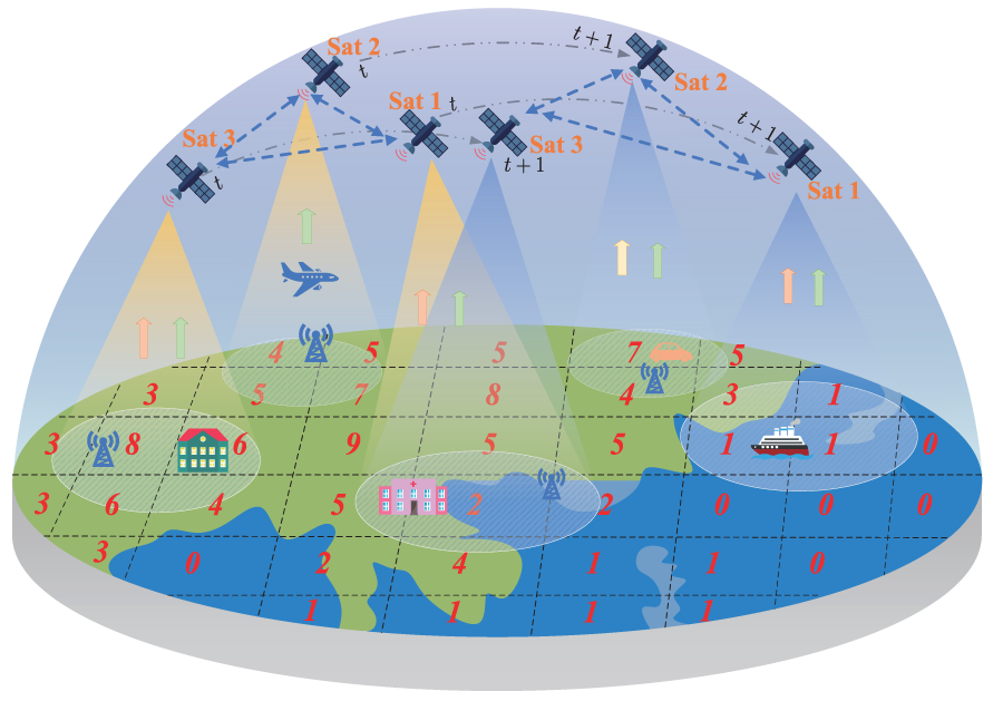
Figure 1: System description of the satellite network.

Multi-granularity traffic

The state of inter-satellite communications is captured by the total traffic matrix Xttotal∈RN×N at time t, which is represented as follows,

Xttotal=[xti,j]i,j=1N(1)

where xti,j is the volume of data transmitted from satellite i to satellite j during the interval (t−1,t]. This matrix represents the traffic volume exchanged between every pair of satellites and provides a global view of the network load distribution.

To capture fine-grained traffic behaviors while preserving a unified network view, the total traffic matrix at time t is decomposed into K service-specific components. The decomposition is represented as follows,

Xttotal=∑k=1KXt(k)(2)

where Xt(k) denotes the traffic matrix corresponding to the k-th service category (e.g., video, IoT.) and K is the number of service types. This fine-grained decomposition not only preserves the structural consistency of the overall network but also enables the model to learn service-aware patterns. Such enriched feature representations benefit both macro-level total traffic prediction and micro-level service-specific prediction.

To predict total satellite traffic at the next time step, the historical traffic data should be used. We consider the latest historical data for input which is represented as follows,

𝒳ttotal = [Xt−T+1total,Xt−T+2total,…,Xttotal](3)

where T denotes the time window of the latest data.

Similarly, For the k-th service traffic, the input sequence is represented as follows,

𝒳t(k) = [Xt−T+1(k),Xt−T+2(k),…,Xt(k)](4)

To perform multi-granularity traffic prediction, the macro-level and micro-level historical sequences are jointly organized as a unified multi-granularity input which is represented as follows,

𝒳t{MG}=[𝒳t{total},𝒳t(1),…,𝒳t(K)](5)

Dynamic inter-satellite distance

Due to continuous orbital motion, inter-satellite distances vary in real time. These variations directly affect signal quality and link stability. As a result, routing strategies and traffic flows must dynamically adapt to the changing spatial topology [25]. When the distance between two satellites approaches the maximum communication range, available bandwidth can drop sharply or be lost altogether. As a result, traffic is rerouted via alternative paths. In contrast, when inter-satellite distances become shorter, the resulting improvements in link quality and throughput can effectively alleviate existing network congestion. Therefore, distance is considered an important factor affecting satellite traffic. It is further used as an auxiliary input to improve the extraction of spatial-temporal dependencies.

The communication distance dti,j between satellites i and j at time t is represented as follows,

dti,j={dti,j,if dti,j≤Rmax−∞,if dti,j>Rmax(6)

where Rmax represents the maximum distance for establishing a communication link between satellites due to the curvature of the Earth and limitations of communication equipment. Based on all pairwise distances, the inter-satellite distance matrix at time t is represented as follows,

Dt=[dti,j]i,j=1N(7)

To assist in predicting satellite traffic at the next time step, the historical inter-satellite distances can be used. We consider the latest historical inter-satellite distances for input which is represented as follows,

𝒟t=[Dt−T+1,Dt−T+2,…,Dt](8)

The sequence 𝒟t can capture short-term geometric variations in the satellite constellation and serve as an auxiliary input to help learn spatial-temporal dependencies of traffic fluctuations caused by satellite mobility.

Dynamic served population

The continuous movement of satellites causes their coverage areas on the ground to shift over time. This results in dynamic changes in both the number of served users and the corresponding traffic load [26]. Traffic demand in satellite networks is closely tied to the size of the covered population. As illustrated in Fig. 1, Sat 1 and Sat 3 cover the same geographical region at different time, which results in a strong correlation between their traffic demands. In particular, when multiple satellites simultaneously or sequentially serve overlapping or adjacent areas, their traffic loads tend to exhibit significant correlation. In regions with high population density, traffic demand across multiple satellites often varies synchronously and tends to exhibit similar fluctuations. The dynamic variation of served population information supports the modeling of spatial-temporal traffic correlations and contributes to improving prediction accuracy. Therefore, population density maps are integrated with satellite beam footprints to derive a dynamic served population representation, which is incorporated as auxiliary input to the prediction model.

The satellite coverage region can be approximated as the ground projection of its antenna beam [27]. Assuming a circular beam footprint, the coverage area Si(t) of satellite i at time t is computed by

Si(t)=2πRe2(1−cos⁡βi(t))(9)

βi(t)=arcsin(hi(t)+ReResin⁡θ)(10)

where Re denotes the Earth’s radius, hi(t) denotes the altitude of satellite i above the ground at time t, θ denotes half-beam angle of the satellite antenna, and βi(t) denotes geocentric half-cone-angle of the coverage region. Based on the coverage area Si(t), the total population served by satellite i at time t can be estimated by

pti=∬(x,y)∈𝒮i(t)p(x,y)dxdy(11)

where p(x,y) is the population density at geographic coordinates (x,y) at time t. This formulation explicitly incorporates the temporal dimension, enabling dynamic estimation of each satellite’s coverage area and the corresponding user population over time.

By aggregating the estimates across all satellites, the served population state at time t is represented as

Pt=[pti]i=1N(12)

To assist in predicting satellite traffic at the next time step, the historical served population information can be utilized. We consider the most recent sequence of served population vectors as input, which is represented as follows

𝒫t=[Pt−T+1,Pt−T+2,…,Pt](13)

The sequence 𝒫t can capture short-term variations in user distribution and serve as an auxiliary input to help learn spatial-temporal dependencies of traffic fluctuations driven by population dynamics.

Based on the above input data, the prediction problem can be represented as follows

Xt+1total,Xt+1(1),…,Xt+1(K)=g(𝒳t{MG},𝒟t,𝒫t;θ)(14)

where Xt+1total denotes the predicted total traffic matrix at time step t+1, Xt+1(k) denotes the predicted traffic matrix for the k-th service type at time t+1 and θ represents the learnable parameters for the prediction model.

3  Multi-Granularity Traffic Prediction Model Based on Dynamic Adaptive Graph Modeling

To achieve multi-granularity satellite traffic prediction, a graph-based model architecture is proposed, which consists of a shared spatial-temporal feature extraction module and task-specific prediction branches. Both global traffic and service-level traffic are derived from the same underlying network topology and population dynamics, therefore a shared feature extractor enables consistent modeling of spatial dependencies and temporal evolution across tasks. This design reduces parameter redundancy and enhances the generalizability of the learned representations. In addition, global and service-level traffic exhibit distinct spatial-temporal characteristics and modeling objectives. Employing a single prediction head for all tasks compromises the model’s capacity to capture fine-grained traffic variations, which may result in suboptimal performance. Hence, the model adopts a modular architecture comprising one macro branch and multiple micro branches.

The overall model parameters θ are divided into three parts. The macro branch focuses on predicting the total network traffic based on historical data. It relies on shared spatial-temporal features and employs independent parameters for total traffic prediction. The prediction function gmacro is

X^t+1total=gmacro(𝒳ttotal, 𝒟t, 𝒫t;θshared,θmacro)(15)

where θshared denotes the shared spatial-temporal feature extraction parameters, and θmacro denotes the macro-branch parameters used for total-traffic prediction. The micro branch is designed to predict traffic for individual service types. Although it shares the spatial-temporal feature extraction module with the macro branch, each service type employs a dedicated set of prediction parameters to capture its unique traffic patterns. The prediction function gmicro is

X^t+1(k)=gmicro(𝒳t(k), 𝒟t, 𝒫t;θshared,θmicro(k))(16)

where θmicro(k) represents its service-specific prediction parameters. This structural design enables the allocation of dedicated parameters to different tasks and enhance prediction flexibility and accuracy.

The proposed multi-granularity traffic prediction model is shown in Fig. 2 which consists of five steps. First, the node feature projection module processes the original multi-source heterogeneous inputs, including traffic, population distribution, and inter-satellite distance. Each modality is transformed by a dedicated weight matrix and nonlinearly projected into a shared latent space to obtain node-level representations from dual perspectives. Second, the node feature embeddings module integrates the projected features through element-wise operations. This produces unified node embeddings that serve as the basis for graph construction. Third, the adjacency matrices construction module computes similarity between node embeddings. It dynamically generates multiple adjacency matrices that reflect spatial relationships from different views and form the dynamic graph structure. Fourth, the spatial correlation modeling module applies graph diffusion convolution. It captures spatial dependencies and aggregates multi-hop neighborhood information to enhance representation capability. Fifth, the temporal correlation modeling module uses gated recurrent units (GRUs) to perform sequence modeling. It fuses the current node input with historical hidden states to extract temporal dynamics. Finally, the model predicts both global traffic and service-level traffic through one macro branch and multiple micro branches. A consistency loss is introduced to enforce alignment between macro and micro predictions, which improves both accuracy and generalization. The details of the model are further introduced below.

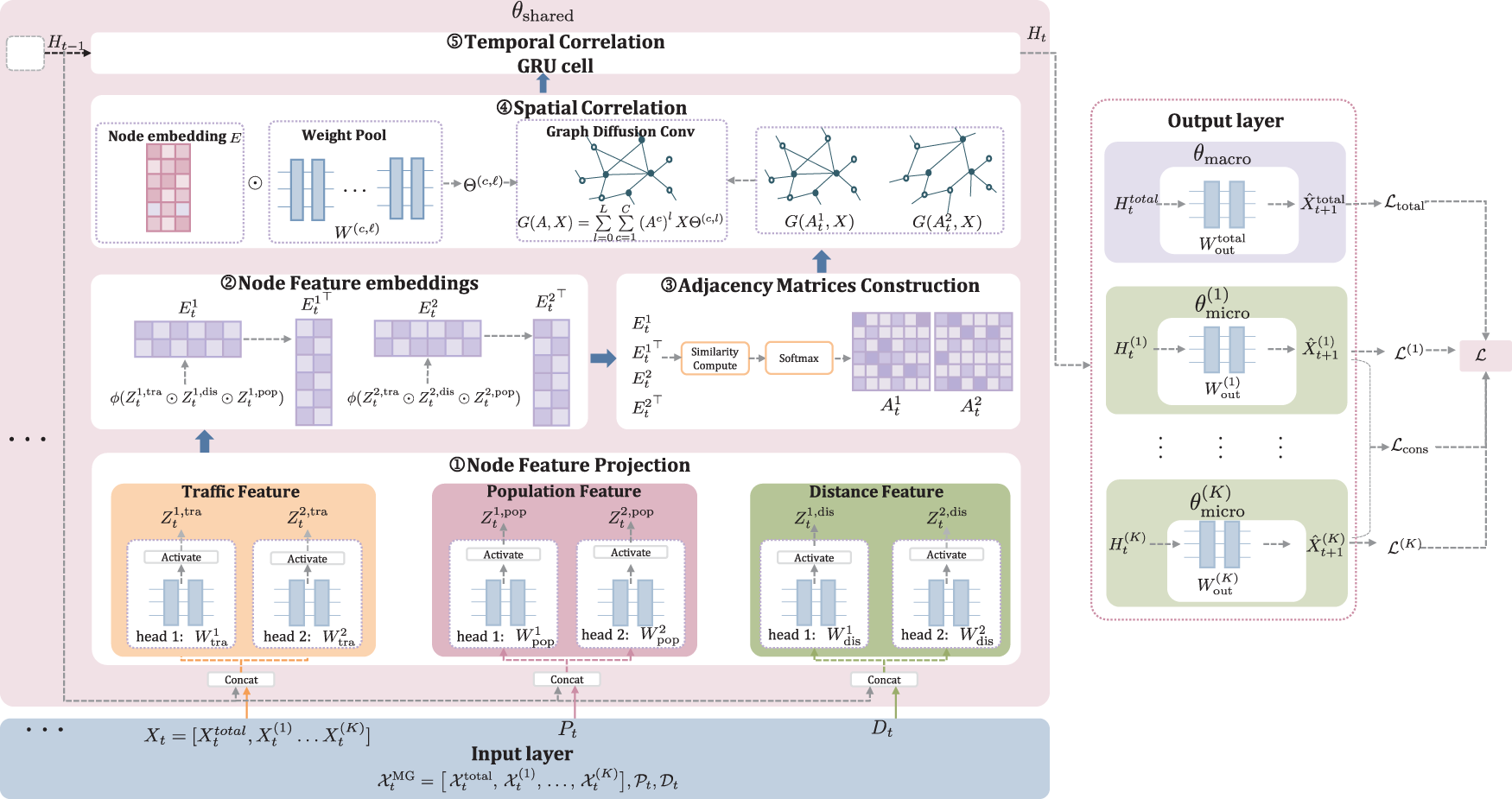
Figure 2: The architecture of the multi-granularity traffic prediction model.

3.1 Node Feature Projection and Embedding

Before training and testing the model, all input features are normalized to ensure numerical stability and consistency across different modalities. This preprocessing step allows the model to focus on relative variations rather than absolute magnitudes. Prophet [24] normalizes each traffic matrix at time t by dividing all elements by its maximum value, thereby mapping the raw traffic intensities into the relative range [0,1]. This approach preserves the spatial structure of the matrix and allows downstream models to effectively capture load disparities across paths. Inspired by this method, the resulting matrix is referred to as the relative load matrix. Specifically, let

Mt=max1≤i,j≤Nxti,j,x~ti,j=xti,jMt,(17)

and define

X~ttotal=[x~ti,j]i,j=1N,(18)

where x~ti,j∈[0,1] with 1 indicating that link (i,j) carries the maximum traffic at time t and 0 indicating no traffic. This normalization eliminates fluctuations in absolute traffic levels across time steps, enabling the model to concentrate on relative intensity patterns and spatial distribution dynamics. To quantify each service’s relative contribution on a given link, a ratio-based normalization is applied to the k-th service traffic on link (i,j):

Sti,j=∑l=1Kxt(l),i,j,x~t(k),i,j=xt(k),i,jSti,j,(19)

with ∑k=1Kx~t(k),i,j=1. The service-specific load ratio matrix is then defined as

X~t(k)=[x~t(k),i,j]i,j=1N(20)

which represents the proportion of total traffic on each link attributed to service k at time t. Similarly, the distance and population matrices are normalized using min-max scaling at each time step, yielding the normalized distance matrix D~t and normalized population vector P~t, which are used as auxiliary inputs to the prediction model.

3.1.1 Node Feature Projection

Link traffic variations in a satellite network are driven not only by the current traffic distribution but also by the constellation’s geometric structure and the ground user density. A single feature mapping cannot fully capture the complex interactions among these three modalities. Hence, the node feature projection module processes the original multi-source heterogeneous inputs, including traffic, population distribution, and inter-satellite distance. Each modality is transformed by a dedicated weight matrix and nonlinearly projected into a shared latent space to obtain node-level representations from dual perspectives.

Traffic projection

To further boost expressive capacity, dual-head parallel projections are introduced during traffic mapping: two channels share the same input but employ independent learnable linear mappings to encode both the global relative-load matrix X~ttotal and the k-th service relative-load matrix X~t(k). Specifically, the projection of head h is given by:

Zth,total,tra=[X~ttotal ‖ Ht−1total]Wtrah(21)

Zth,(k),tra=[X~t(k) ‖ Ht−1(k)]Wtrah(22)

where Ht−1total and Ht−1(k) denote the node representations generated by the GRU cell at time t−1, the operator [⋅ ‖ ⋅] denotes the concatenation of two feature matrices along the feature dimension and Wtrah is the learnable projection matrix of head head h. h∈{1,2} indexes the two parallel linear mapping channels. This dual-head configuration enables the model to capture a richer set of feature representations.

Population projection

To incorporate temporal context into static population information, the normalized population vector P~t is concatenated with the GRU hidden state and projected as:

Zth,total,pop=[P~t ‖ Ht−1total]Wpoph(23)

Zth,(k),pop=[P~t ‖ Ht−1(k)]Wpoph(24)

where Wpoph are learnable weight matrices.

Distance projection

Similarly, the normalized inter-node distance matrix D~t is projected using a temporal-aware mapping:

Zth,total,dis=[D~t ‖ Ht−1total]Wdish(25)

Zth,(k),dis=[D~t ‖ Ht−1(k)]Wdish(26)

where Wdish are learnable weight matrices.

The learnable parameters for the node feature embedding module are:

Θprojected={Wtrah, Wdish, Wpoph}for all h∈{1,2}(27)

3.1.2 Node Feature Embeddings

The node feature embeddings module integrates the projected features from different modalities through element-wise operations. This yields unified node representations that serve as the foundation for graph construction. Specifically, each traffic projection is fused with its corresponding distance and population projections via element-wise multiplication ⊙ (i.e., the Hadamard product). The fused representation is then passed through a nonlinear activation function ϕ(⋅), such as tanh.

Eth,total=ϕ(Zth,total,tra⊙Zth,total,dis⊙Zth,total,pop)(28)

Eth,(k)=ϕ(Zth,(k),tra⊙Zth,(k),dis⊙Zth,(k),pop)(29)

After dual-head fusion, the final node embeddings are generated by vertically stacking the outputs from the two heads, resulting in a unified representation for each node that integrates complementary directional and modal information. Specifically, the global traffic and service-specific embeddings are constructed as follows:

Ettotal=[Et1,totalEt2,total],Et(k)=[Et1,(k)Et2,(k)](30)

These embeddings represent two complementary views of each node at time t, capturing both directional dependencies and heterogeneous traffic semantics. The resulting representations are then forwarded to the dynamic adjacency matrix construction module to model pairwise node interactions. This enriched embedding space facilitates the learning of bidirectional and multimodal spatial dependencies, serving as input for subsequent graph diffusion and temporal reasoning stages.

3.2 Dynamic Adaptive Adjacency Matrix Construction

Based on the fused node feature embeddings, the adjacency matrices construction module computes pairwise similarities to capture spatial relationships between nodes. Specifically, a pair of direction-aware similarity matrices is constructed by calculating the inner-product differences between dual-head embeddings. This design leverages the asymmetry and complementarity of dual views to model heterogeneous spatial dependencies more effectively. The choice of inner-product differences over widely used alternatives (i.e., cosine similarity and attention-based methods) is motivated by the unique characteristics of satellite network traffic prediction, as elaborated below.

First, cosine similarity is not adopted because it inherently yields a symmetric matrix, which incorrectly treats asymmetric node interactions as having equal strength and thus masks the unidirectional transmission characteristic of satellite network traffic. In satellite network link traffic prediction, spatial interactions between nodes exhibit strict directionality and asymmetry—for instance, the data transfer intensity from satellite i to satellite j may be much higher than that in the reverse direction (satellite j to satellite i). Such symmetry would mislead the subsequent graph convolution module into failing to capture the true spatial dependencies. In contrast, inner-product differences create an antisymmetric matrix that quantifies the difference in interaction strength between the two directions in the satellite network.

Second, attention-based methods are not selected despite their adaptability, as they typically introduce additional projections and higher computational overhead. Attention mechanisms rely on learnable query/key projection matrices to implicitly model node dependencies, and these extra projection parameters increase the model’s computational complexity and parameter burden. Since the dynamic graph needs to be updated at each time step, computing attention weights across all node pairs at each step would elevate the cost of dynamic graph construction.

The resulting dynamic adjacency matrices reflect both the similarity and interaction strength between nodes. They enable bidirectional and multi-modal spatial modeling in subsequent graph convolution stages, serving as the structural backbone for dynamic graph construction.

Specifically, for the global traffic embeddings, the head-wise similarity matrix is defined as:

Δttotal=Et1,total⋅(Et2,total)⊤−Et2,total⋅(Et1,total)⊤(31)

For the k-th service-specific embeddings, the asymmetric similarity matrix is:

Δt(k)=Et1,(k)⋅(Et2,(k))⊤−Et2,(k)⋅(Et1,(k))⊤(32)

To preserve the directional distinction and filter out negative interactions, a nonlinear activation function ϕ(⋅) (e.g., ReLU or tanh) is applied to both the forward and reverse components of each similarity-difference matrix. The results are then normalized row-wise using softmax to obtain two directional dynamic adjacency matrices. For the global traffic embedding, the resulting adjacency matrices are:

Attotal=[At1,totalAt2,total]=[softmax(ϕ(Δttotal))softmax(ϕ(−Δttotal))](33)

For the k-th service traffic embedding, the two-view adjacency matrices are:

At(k)=[softmax(ϕ(Δt(k)))softmax(ϕ(−Δt(k)))](34)

where softmax(⋅) is applied row-wise to ensure each node’s outgoing edge weights form a valid probability distribution. The matrices At1,total and At2,total (as well as At1,(k) and At2,(k) for each service k) together form the two-view directional adjacency matrices, which are then forwarded into the graph diffusion convolution and temporal modeling modules.

3.3 Spatial-Temporal Correlation Modeling

Satellite network traffic exhibits significant spatial-temporal dependencies. The approach that combines Graph Diffusion Convolution (GDC) with Gated Recurrent Units (GRU) can effectively capture the spatial-temporal features of the input sequences [28]. GDC aggregates multi-hop neighborhood information to form spatial representations that reflect dynamic topology. The spatial features are subsequently processed by GRU units to model both short-term and long-term temporal dynamics within a unified framework. Based on this method, we propose a dynamic adaptive graph model that fuses population coverage, inter-satellite distances, and historical traffic data into the adjacency structure. The constructed dynamic graphs are fed into both the GDC and GRU components to extract robust spatial-temporal representations.

3.3.1 Spatial Correlation

Given the input node feature matrix X∈RN×d and the set of multi-channel adjacency matrices A=[A1,A2,…,AC], the spatial dependency is modeled using GDC [29]:

G(A,X)=∑l=0L∑c=1C(Ac)lXΘ(c,l)(35)

where C is the number of adjacency matrix channels and L is the diffusion order.

To incorporate node-specific adaptive transformations, element-wise modulation is applied to the weight pool.

Θ(c,l)=E⊙W(c,l)(36)

where E∈RN×d is the node adaptive embedding matrix, W(c,l) is the weight pool corresponding to the l-th order diffusion of the c-th channel.

The full parameter set of the spatial convolution module is

ΘGDC={W(Ci,Lj) | Ci=1,…,C; Lj=0,…,L}(37)

3.3.2 Temporal Correlation

Given input (At,Xt,Ht−1) at time t, temporal modeling is performed via a GRU cell integrated with graph convolution operations:

zt=σ(G(z)(At,[Xt‖Ht−1])),rt=σ(G(r)(At,[Xt‖Ht−1])),h~t=tanh⁡(G(h)(At,[Xt‖(rt⊙Ht−1)])),Ht=zt⊙Ht−1+(1−zt)⊙h~t(38)

where σ(⋅) is the sigmoid activation, ‖ denotes feature concatenation, and G(⋅) is a graph convolution (same form as above) specific to the gate or hidden state. zt and rt are the update and reset gates, respectively, while h~t is the candidate state.

Both the total-traffic and per-service features are fed into GRUs to generate their respective hidden representations:

Httotal=GRU(Xttotal,Attotal,Ht−1total)(39)

Ht(k)=GRU(Xt(k),At(k),Ht−1(k))(40)

These outputs serve as spatial-temporal node embeddings, providing dynamic, service-aware representations for prediction tasks. Each GRU gate is associated with an independent GDC module. Therefore, the parameter set of the GRU-based spatial-temporal modeling is

ΘGRU=(ΘGDC(z),ΘGDC(r),ΘGDC(h))(41)

where ΘGDC(⋅) denotes the GDC parameters used for the update gate, reset gate, and candidate state.

The set of shared model parameters is defined as

θshared={Θprojected,ΘGRU}(42)

which is jointly optimized across both macro-level and micro-level prediction branches to enable consistent spatial-temporal representation learning.

3.4 Multi-Granularity Prediction with Consistency Regularization

The proposed macro-micro dual-branch architecture is designed to balance the trade-off between learning common spatial-temporal dynamics and preserving service-specific characteristics. A key challenge in multi-granularity prediction is the potential conflict between feature patterns of different service types. While services exhibit unique characteristics (e.g., burstiness of video, periodicity of IoT), they are fundamentally governed by common underlying dynamics, such as satellite mobility, topology evolution, and regional user distribution. These common dynamics are captured by a shared spatial-temporal feature backbone. This shared module learns universal representations and prevents redundant modeling of these common factors. Service-specific variations are then isolated and refined by lightweight, independent micro-branch heads. It prevents service-unique signals from interfering with the learning of universal spatial-temporal patterns, thereby striking a balance between efficient representation learning and the preservation of service characteristics. Based on the shared spatial-temporal feature extraction, the model generates macro-level predictions for global traffic and micro-level predictions for each service traffic. The total traffic at time t+1 is predicted by

X^t+1total=HttotalWouttotal(43)

For each service type k∈{1,…,K}, the traffic at time t+1 is predicted by

X^t+1(k)=Ht(k)Wout(k),k=1,…,K(44)

The parameters of macro prediction branch are defined as

θmacro={Wouttotal}(45)

Similarly, the parameters of micro prediction branch are defined as

θmicro={Wout(k)∣k=1,…,K}(46)

To capture proportional variations and directional trends in satellite traffic data, an angle loss function [24] is employed as the prediction metric. Given two flow vectors x,y∈RF, the loss function is defined as

f(x,y)=1−xTy‖x‖2‖y‖2(47)

The loss emphasizes the relative orientation between the predicted and true traffic vectors. By ignoring absolute magnitudes, it enables the model to capture proportional variations and directional trends in traffic patterns. The model is trained by minimizing a composite loss function that includes three components: the global traffic prediction loss, the service traffic prediction loss and a consistency regularization term. The overall loss is defined as

ℒ=ℒtotal+ℒsvc+λℒcons(48)

where λ is a hyperparameter balancing the contribution of the consistency term.

The first term ℒtotal measures the discrepancy between the predicted and ground-truth total traffic at time step t+1 and computed by

ℒtotal=f(X^t+1total,Xt+1total)(49)

The second term ℒsvc is total service-level loss. For each service k, the corresponding prediction loss is

ℒ(k)=f(X^t+1(k),Xt+1(k))(50)

and the total service loss is computed by

ℒsvc=∑k=1Kℒ(k)(51)

The third term ℒcons is a consistency regularization loss designed to ensure coherence between the macro-level and micro-level predictions. It compares the predicted total traffic with the sum of all service-level predictions to encourage flow conservation across granularities. The loss is computed by

ℒcons=f(Xt+1total, ∑k=1KX^t+1(k))(52)

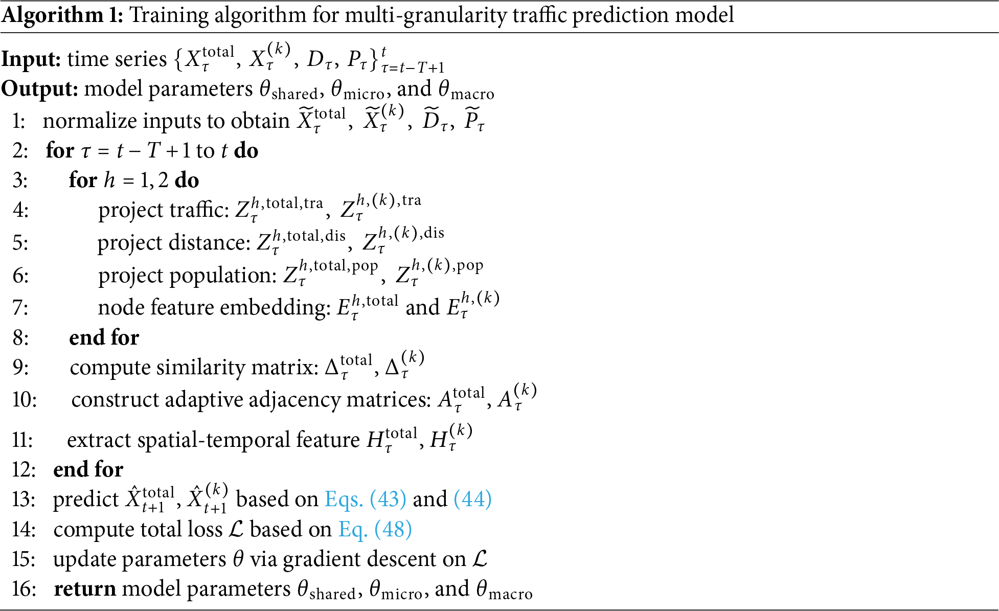
This term penalizes deviations between the aggregated micro predictions and the total traffic ground truth. It encourages structural alignment between the two prediction levels and helps improve overall prediction accuracy. The entire training process involves sequentially processing historical time steps to extract spatial-temporal representations, generating macro and micro predictions, and optimizing the model parameters via gradient-based learning. At each step, multi-modal features are projected and embedded, similarity-based dynamic graphs are constructed, and spatial-temporal representations are updated recursively. The final predictions are compared with ground-truth data using the composite loss function described above, and the parameters are updated accordingly. The detailed procedure is summarized in Algorithm 1.

3.5 Computational Complexity Analysis

For the single-task single-time-step case, the model’s computational complexity primarily arises from graph convolution operations, Gated Recurrent Unit (GRU) operations, and the final traffic prediction step. Specifically, the complexity of the graph convolution is O(N2), the complexity of the GRU operation is O(N), and the complexity of the final prediction is O(N2). Therefore, the overall computational complexity for the single-task single-time-step case can be expressed as O(N2). When extended to the multi-time-step case, where the input consists of the past T time steps of traffic data, the complexity of the graph convolution and GRU operations becomes O(T⋅N2) and O(T⋅N), respectively. The final prediction complexity is O(T⋅N2). Thus, the computational complexity for multiple time steps is O(T⋅N2). In the multi-task case, assuming there are K service types and one global (macro-level) task, the total number of tasks is K+1. For each task, the computational complexity is O(N2), so the overall computational complexity for multi-task multi-time-step prediction is O((K+1)⋅T⋅N2). In summary, the computational complexity of the model is primarily dependent on the number of satellites N and the number of service types K. The computational complexity of the model grows quadratically with the number of satellites N and linearly with the number of service types K.

4  Numerical Results

4.1 Parameter Settings

Based on the proposed multi-granularity model, we assess its performance in a scenario comprising 66 satellite nodes deployed in low Earth orbit. Each satellite has four neighboring nodes. The simulation duration is set to one month. The detailed hyperparameter settings for model training are presented in Table 1. The proposed traffic prediction model supports two deployment options. First, the model can be deployed on ground stations. In this configuration, satellite traffic data is transmitted via satellite-ground communication links for predictions. Second, the model can be deployed on satellites using an offline training and online inference paradigm. Considering the limited on-board resources of satellites, it may be challenging to implement traffic prediction directly on orbit. We conducted research on the current satellite computing performance. For example, each satellite in China’s Three-Body Computing Constellation has an onboard computing capability of up to 744 TOPS, and the constellation targets a total computing power of 1000 POPS, demonstrating significant on-orbit AI compute potential [30]. Additionally, Starcloud-1, launched on 02 November 2025, is an experimental orbiting computation satellite developed by Starcloud, Inc. It carries an NVIDIA H100 GPU and represents a significant advancement in space-based compute capability compared to previous in-orbit systems [31]. The proposed model requires 28.25 MFLOPs for one forward pass of inference. Hence, as the computing power of satellites continues to improve, the proposed algorithm is technically feasible for on-orbit implementation and operation.

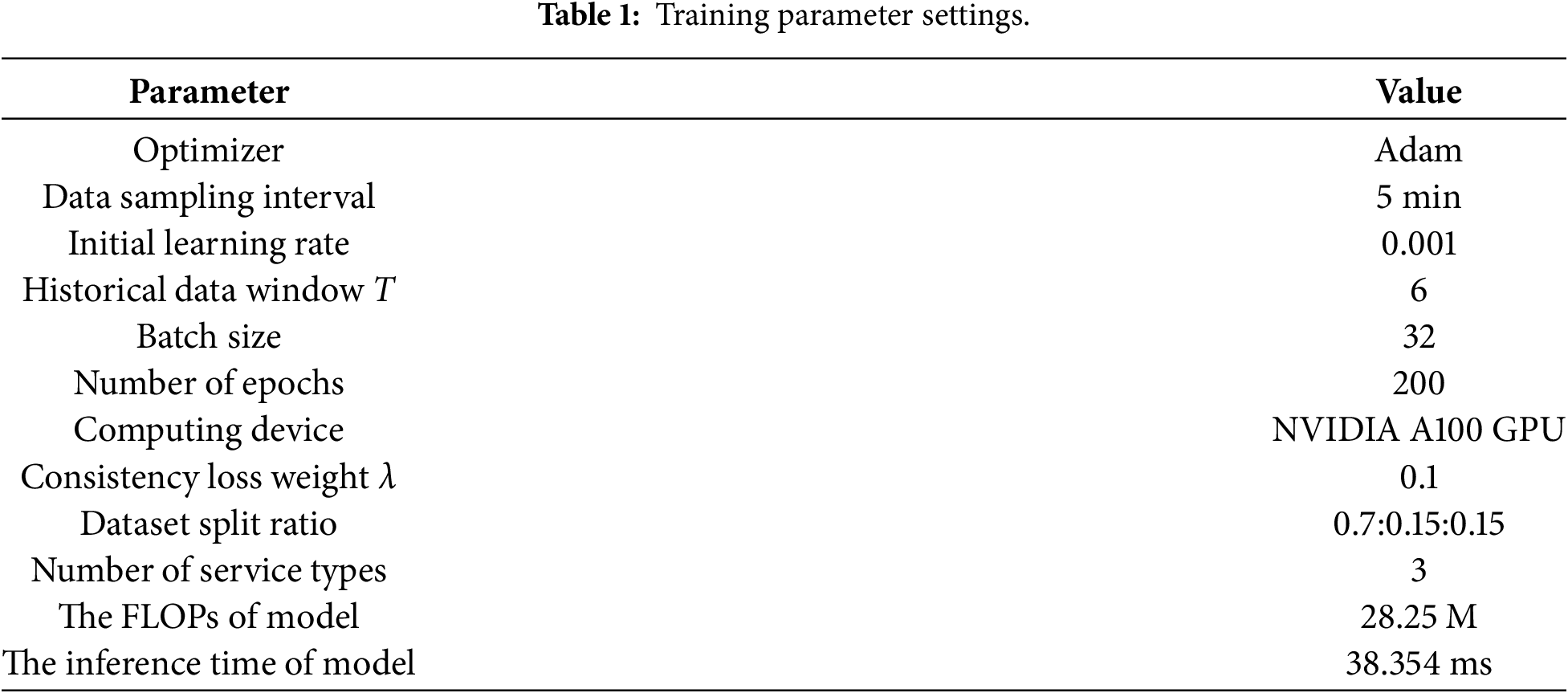
The proposed traffic prediction model has a single inference time of only 37.439 ms, which allows it to predict the traffic state for the next time slot. The existing routing strategies are typically updated based on fixed time slots, which means that route decisions are refreshed at regular intervals [32,33]. Since the predicted time slot aligns with the routing update time slot and the model’s inference time is short, this traffic prediction capability matches the time requirements for routing updates.

4.2 Dataset

Due to the lack of publicly available real-world satellite traffic datasets, traffic generation is simulated based on representative characteristics of service distribution. The geographic partitioning strategy in [34] divides the Earth’s surface into 12×24=288 regions, and population data is available for each region. A ground station is deployed in every region. Each ground station serves a regional user cluster that has a relatively stable communication demand. Since most traffic is handled by terrestrial infrastructure and only a small portion requires satellite relaying, it is assumed that approximately 5% of ground station traffic is forwarded via satellite links [35]. The traffic demand of ground station g at time t is modeled as:

Cg(t)=ελgγ(t)(53)

where ε=0.05 denotes the proportion of traffic requiring satellite transmission, λg is the number of users within the coverage of station g (in units of 106), and γ(t) is a temporal modulation factor that captures diurnal variation in demand. Service types are indexed by k=1,2,…,K, and the generation probability of service type k at time t is denoted as πk(t). The day is divided into four periods: 00:00–08:00, 08:00–18:00, 18:00–22:00, and 22:00–24:00. The probability proportions of generated traffic for the three service types in these periods are set to 0.1:0.1:0.8, 0.4:0.5:0.1, 0.6:0.3:0.1, and 0.1:0.1:0.8, respectively. The demand for service k generated by ground station g at time t is given by:

Cgk(t)=πk(t)⋅Cg(t)(54)

The set of ground stations covered by satellite i at time t is denoted as 𝒢i. The total amount of type-k traffic received by satellite i is calculated as:

xik(t)=∑g∈𝒢iCgk(t)(55)

To support multi-hop routing in the satellite network, a gravity-inspired traffic splitting mechanism is applied. The set Ω represents the neighbors of satellite i that are reachable for data forwarding. The proportion of type-k traffic forwarded from satellite i to satellite j∈Ω is determined by:

xijk(t)=xik(t)⋅xjk(t)/dtij∑q∈Ωxqk(t)/dtiq(56)

where dtij is the distance between satellites i and j at time t. The total traffic transmitted from node i to node j is obtained by summing across all service types:

xij(t)=∑k=1Kxijk(t)(57)

This modeling framework incorporates population distribution, temporal variability, spatial topology, and coverage constraints, and results in a synthetic satellite network dataset.

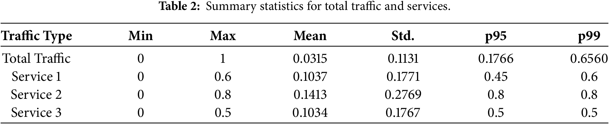
To provide a comprehensive view of the generated dataset’s characteristics, Table 2 presents summary statistics for both total traffic and individual service traffic after normalization. Statistics metrics include the minimum (min), maximum (max), mean, standard deviation (std), 95th percentile (p95), and 99th percentile (p99) for each traffic type. These statistics reveal several key properties that define the inherent challenge of multi-granularity prediction. First, a significant scale difference exists between total and service-level traffic due to distinct normalization strategies. During preprocessing, total traffic undergoes max-normalization, where each element is divided by the maximum traffic value across the entire network at that time step. In contrast, service-level traffic undergoes ratio-normalization, where each service’s traffic is divided by the sum of all service traffic on its corresponding link. Consequently, service-level traffic exhibits mean values 3–5 times larger than total traffic. Furthermore, service-level data shows greater intrinsic volatility, with standard deviations 1.6–2.5 times higher than those of total traffic. Second, the statistics highlight the heterogeneous characteristics inherent in each service’s traffic pattern. As shown in Table 2, Service 2 exhibits the most challenging statistical profile. It has the highest mean (0.1412), the highest standard deviation (0.2769), and the most concentrated extreme-value distribution. These characteristics indicate that Service 2 has the most unstable traffic pattern, which makes it inherently the most difficult service to predict. In contrast, Services 1 and 3 show more moderate and similar statistical profiles. Together, these properties establish the fundamental complexity of jointly predicting total network load and fine-grained service-level traffic, which motivates the design of a multi-granularity modeling framework.

4.3 Evaluation Metrics

To comprehensively assess model performance, we employ both error-based and correlation-based metrics: MAE (Mean Absolute Error) and RMSE (Root Mean Square Error) are used to measure the numerical deviation between predictions and ground truths. These metrics quantify the absolute and squared errors, respectively, and smaller values indicate better performance. CORR (Pearson Correlation Coefficient) and COS (Cosine Similarity) are used to evaluate the consistency of variation trends between predicted and true traffic patterns. Higher values of these metrics suggest stronger correlation and alignment in the overall distribution.

4.4 Results Analysis

4.4.1 Performance Evaluation of the Proposed Model

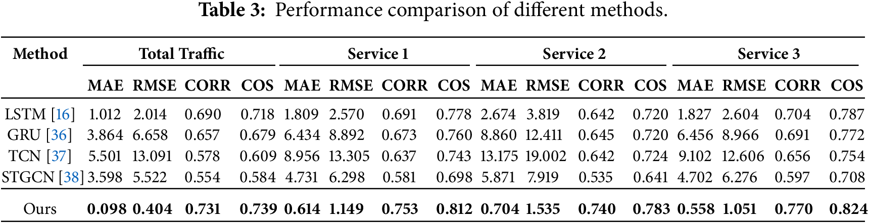
To evaluate the effectiveness of the proposed model in capturing the spatial-temporal correlations of traffic flow, we conducted comparative experiments against several representative baseline methods, including conventional sequence modeling approaches (e.g., LSTM [16] and GRU [36]), a convolution-based model (TCN [37]), and a graph-based spatial-temporal model (STGCN) [38]. To ensure a fair comparison, all methods were implemented under a unified multi-task prediction framework and trained using our proposed multi-granularity loss function, which enables consistent optimization objectives across different models. As shown in Table 3, the proposed model consistently outperforms all baselines across all evaluation metrics. The proposed model constructs dynamic and adaptive adjacency matrices from multi-source features and uses a parameter-sharing mechanism to extract spatial-temporal features. In particular, our model achieves a cosine similarity of 0.739 for total traffic prediction, which is significantly higher than those of LSTM, GRU, and STGCN. This result demonstrates its superior capability in modeling traffic distribution proportions. LSTM and GRU capture only temporal sequences and ignore spatial connectivity. Their total traffic MAEs exceed 1.0 and RMSEs exceed 2.0. The COS of LSTM is 0.02 lower than that of our model, and the COS of GRU is 0.05 lower than that of our model. These results demonstrate that relying solely on temporal dependencies is insufficient, and that integrating spatial connectivity is essential for accurate traffic prediction. TCN enhances temporal feature extraction but cannot leverage dynamic graph structures. It yields MAEs as high as 5.501 and RMSEs of 13.091. The COS of TCN is 0.13 lower than that of our model. STGCN introduces graph convolutions but relies on a static adjacency matrix and achieves only a CORR of 0.554 and a COS of 0.584. In summary, the experimental results demonstrate the effectiveness of the proposed model in learning complex spatial-temporal dependencies and enhancing multi-task traffic prediction performance.

4.4.2 Performance Evaluation of Different Features

This experiment evaluates the performance of various models for traffic prediction in a satellite network, focusing on the impact of population and distance features on the prediction accuracy. The following models are compared:

•   TP-T: the traffic prediction model using only traffic data for prediction.

•   TP-T-P: the traffic prediction model incorporating traffic data and population features.

•   TP-T-D: the traffic prediction model incorporating traffic data and distance features.

•   TP-T-P-D: the traffic prediction model using traffic data, population features, and distance features.

The results reveal that integrating population and distance features improves prediction accuracy, especially for tasks with more pronounced spatial-temporal dependencies. From Fig. 3, it is evident that TP-T-P-D consistently outperforms the other models across all tasks, with significant improvements in both CORR and COS metrics. Specifically, the inclusion of population data helps account for regional user distribution, while distance features provide critical geographical context, both of which lead to more accurate predictions. These findings highlight the critical role that population and distance features play in capturing the spatial-temporal dependencies of traffic patterns, especially in satellite networks where both geographical and demographic factors are crucial for accurate forecasting.

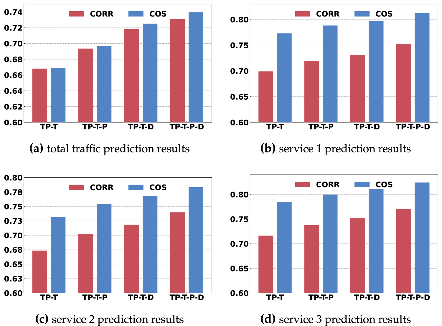
Figure 3: The effect of population and distance features in traffic prediction.

4.4.3 Performance Evaluation of Multi-Granularity Models

Comparative experiments between single-granularity and multi-granularity models are conducted to assess the effectiveness of multi-granularity joint optimization in integrated satellite network traffic prediction. The single-granularity model is optimized solely based on the prediction loss for one service traffic type, whereas the multi-granularity model further integrates multiple task-specific losses and a consistency regularization term to capture both global traffic trends and fine-grained service characteristics. During testing, the cosine similarity between predicted and true vectors is calculated and corresponding histograms and kernel density estimation (KDE) curves are generated. Fig. 4 presents the distributions of cosine similarity (shown as histograms) and the corresponding kernel density estimation (KDE) curves on testset samples for total traffic (a) and for individual services (b–d). In Fig. 4, the horizontal axis denotes the cosine similarity between predicted and true traffic vectors, and higher values indicate better alignment. The vertical axis represents the sample density. Superior models exhibit distributions shifted toward higher cosine similarity and reduced density in the lower-similarity region. Compared with the single-granularity model, the multi-granularity model’s distribution is notably shifted toward higher similarity values and shows reduced density in the lower-similarity region. This shift reflects its ability to produce accurate traffic predictions. This enhancement is attributed to the multi-granularity framework’s ability to model macro-level temporal dependencies in its main branch, leverage auxiliary task branches for service-level details, and align macro-level and micro-level features via consistency loss, thereby enabling more comprehensive spatial-temporal correlation modeling.

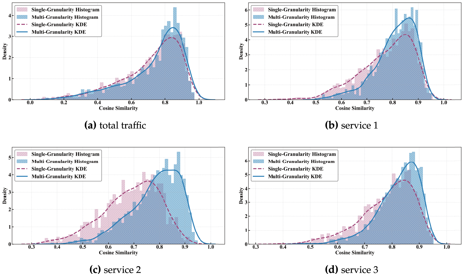
Figure 4: Comparison of cosine similarity distributions and KDE curves between single-granularity and multi-granularity models.

4.4.4 Generalization Verification of the Proposed Model

To evaluate the generalization capability of the proposed model under various satellite network scenarios, experiments are conducted on two key parameters: constellation size (with N=66,72,84) and the proportion of satellite traffic (with ε=5%,8%,10%). As illustrated in Fig. 5a, when the number of satellite nodes increased from 66 to 84, the model’s CORR remained stable within the range of 0.83–0.85 (a fluctuation of 2.4%), while COS varied between 0.87–0.89 (a fluctuation of 2.3%). This demonstrates that the model maintains consistent performance across different constellation scales. It indicates that the dynamically adaptive graph modeling approach effectively accommodates the expansion of network topology. Even with an increase in the number of satellites, the model continues to accurately capture spatial dependencies by constructing adjacency matrices through the integration of population and distance features. Similarly, as illustrated in Fig. 5b, when the traffic proportion increased from 5% to 10%, CORR values stayed within 0.83–0.84 (a fluctuation of 1.2%), and COS ranged from 0.87 to 0.88 (a fluctuation of 1.1%). Overall, the model’s performance remained stable across variations in constellation size and traffic proportion.

Figure 5: Model performance comparison under different scenario parameters. (a) the CORR and COS values with different constellation sizes (N=66,72,84); (b) the CORR and COS values with different satellite traffic proportions (ε=5%,8%,10%).

To validate the model’s adaptability to data uncertainty in real-world scenarios, Gaussian noise was applied to the population coverage features at varying levels from 0% to 30%. As illustrated in the Fig. 6, the model demonstrates robustness in prediction performance. The CORR consistently remains within a high range of 0.843–0.879, while COS stays stable between 0.896 and 0.919. Notably, at a moderate noise level of 15%, both CORR and COS reach their peak values of 0.879 and 0.919, respectively. This suggests that an appropriate level of noise may enhance the model’s generalization ability through implicit regularization. Even when noise increases to 30%, performance shows no significant degradation, with CORR at 0.843 and COS at 0.897. This indicates that the model’s decision-making does not overly rely on the precise values of specific features but instead captures more fundamental traffic evolution patterns through the shared spatial-temporal feature extraction and graph diffusion mechanisms. This confirms that the proposed framework can effectively handle inaccuracies in population data estimation in real satellite networks and demonstrates engineering practicality.

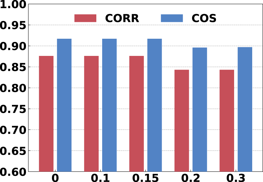
Figure 6: Performance under different noise levels.

4.4.5 Sensitivity Analysis of Hyperparameters

To quantify the role of the consistency loss in balancing flow conservation and prediction accuracy, we fix all other hyperparameters and evaluate λ = 0.00, 0.05, 0.10, and 0.20. As shown in Fig. 7, the RMSE, MAE, CORR, and COS on the test set are compared. As λ increases from 0.00 to 0.10, RMSE and MAE decrease steadily while CORR and COS improve markedly. This demonstrates that moderate consistency regularization effectively links service-specific branches to the global prediction, enforces flow conservation, and enhances both stability and accuracy. When λ increases to 0.20, RMSE and MAE rise and CORR and COS fall. This pattern shows that an overly strong consistency constraint impedes the model’s ability to fit the original observations. Overall, λ = 0.10 achieves the optimal trade-off between accurate forecasting and flow conservation. These findings confirm that the consistency loss plays a important role in our multi-granularity framework by blending macro-level trends with micro-level details, thereby improving model generalization and robustness.

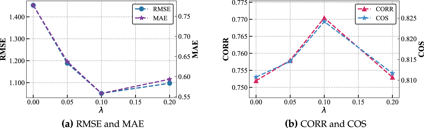
Figure 7: The effect of consistency-loss weight λ.

In addition to the analysis of the consistency loss weight λ, we expanded the exploration to other key hyperparameters, including the diffusion order L and the number of heads H. These parameters play a critical role in shaping the model’s ability to capture both spatial-temporal dependencies and fine-grained features. As shown in Fig. 8a, with the diffusion order L increases from 0 to 2, the model shows a clear improvement in capturing spatial-temporal dependencies, with both CORR and COS rising accordingly. In particular, when L=2, the model achieves an optimal balance between accuracy and stability. This suggests that a moderate diffusion order facilitates the extraction of effective spatial features at multiple scales. However, further increasing the diffusion order to L=3 and L=4 leads to a decline in performance. When L=4, CORR and COS drop significantly. This indicates that an excessively high diffusion order may cause the model to overfit and reduce the model’s generalization ability. Similarly, as illustrated in Fig. 8b, the model’s performance improves markedly as the number of heads increases from 1 to 2, with both CORR and COS rising accordingly. The superior performance of the configuration with H=2 suggests that two heads are optimal for capturing multi-scale spatial dependencies and thereby enhancing predictive capability. However, performance declines when the number of heads is increased to 3 and 4. This drop is particularly noticeable at H=4, where both CORR and COS show a marked decrease. These results suggest that while adding heads can improve performance up to a point, an excessive number may introduce complexity that leads to overfitting and reduced computational efficiency, ultimately impairing predictive effectiveness.

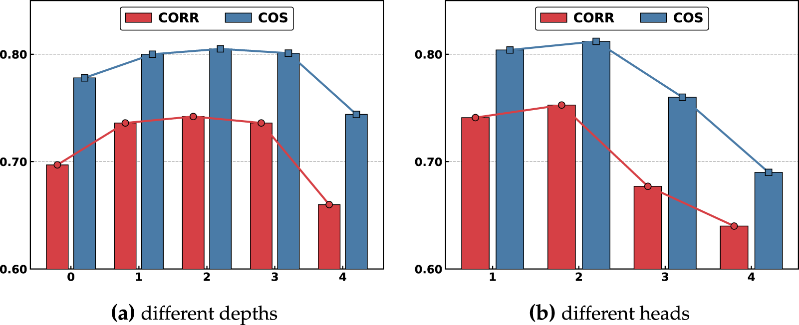
Figure 8: Comparison of model performance with different depths and heads. (a) Performance with different network depths; (b) Performance with different number of heads.

4.4.6 Evaluation of Multi Service Traffic Composition Prediction

To evaluate the model’s ability to accurately estimate the distribution of different service types on each communication link, the predicted and ground-truth proportions for three services are visualized and compared. Ground Truth denotes the actual traffic distribution of Service 1, Service 2, and Service 3 on each link. Multi-Granularity denotes the multi-granularity model proposed in this paper. It employs a macro branch to predict total traffic and three micro branches to predict each service independently. The model is trained using a consistency loss. Single-Granularity denotes the model that uses the same spatio-temporal feature extractor but employs a single prediction branch to estimate total traffic or service-level traffic. The outputs are concatenated without any joint cross-granularity optimization. Fig. 9 shows the distribution of three service types on two communication links, where the y-axis represents each service’s proportion as the height of stacked bars. On both links, the Multi-Granularity bars virtually overlap the Ground Truth. Both the total bar heights and the individual service segment proportions align precisely with the actual distributions. This shows that the model captures global trends and service-level details simultaneously. In contrast, the Single-Granularity bars deviate markedly. In Fig. 9a, the model predicts only Service 2, with Services 1 and 3 almost entirely omitted. In Fig. 9b, Service 1 is roughly estimated but another service’s share is greatly overestimated. These results confirm that simply concatenating separate service predictors fails to integrate macro-level and micro-level information and leads to the omission of low-volume services. The multi-granularity model integrates macro and micro branches under consistency constraints to accurately reproduce each service’s true proportions across diverse scenarios.

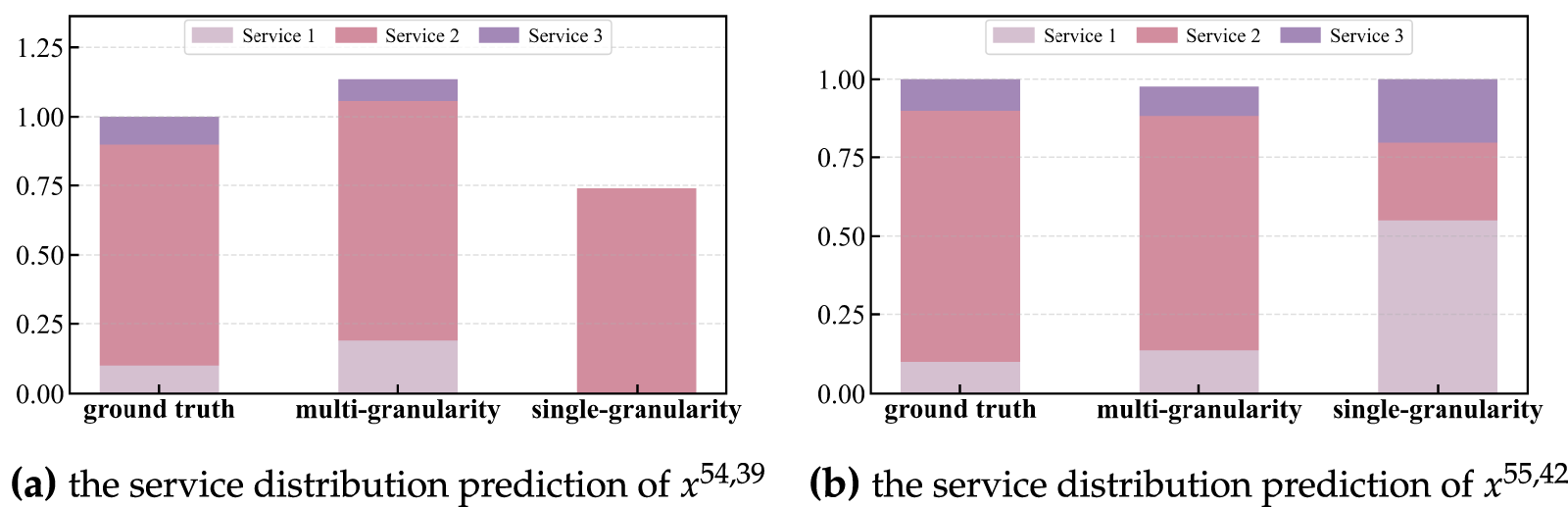
Figure 9: Prediction of service composition over network links.

5  Conclusion

In this paper, a multi-granularity traffic prediction framework for satellite networks based on a shared feature extraction is proposed to benefit from common representations and reduce redundant model parameters. Population coverage, inter satellite distance, and historical traffic data are integrated to capture spatial-temporal dependencies. A multi-task loss function is proposed to jointly optimize predictions of total network traffic and service-level traffic in satellite networks. Experimental results demonstrate that integrating population and distance features improves prediction accuracy. The proposed method outperforms baseline methods and presents its effectiveness in capturing the characteristics of satellite network traffic.

Acknowledgement: The authors would like to thank Nanjing University of Science and Technology.

Funding Statement: This paper was supported in part by National Natural Science Foundation of China under grants U21B2003 and 62103191, and in part by the Fundamental Research Funds for the Central Universities under grant 30924010928.

Author Contributions: Xu Chen and Guohao Qiu: Investigation, Data Curation, Writing—Original Draft, Review and Editing, Visualization. Li Yang: Writing—Review and Editing, Supervision, Funding Acquisition. All authors reviewed and approved the final version of the manuscript.

Availability of Data and Materials: The source code for the proposed method is publicly available on GitHub: https://github.com/cx5055/mg-trafficprediction.

Ethics Approval: Not applicable.

Conflicts of Interest: The authors declare no conflicts of interest.

References

1. Kato N, Fadlullah ZM, Tang F, Mao B, Tani S, Okamura A, et al. Optimizing space-air-ground integrated networks by artificial intelligence. IEEE Wirel Commun. 2019;26(4):140–7. doi:10.1109/mwc.2018.1800365. [Google Scholar] [CrossRef]

2. Liu Z, Gui Y, Wang L, Jiang Y. Offload strategy for edge computing in satellite networks based on software defined network. Comput Mater Contin. 2025;82(1):863–79. doi:10.32604/cmc.2024.057353. [Google Scholar] [CrossRef]

3. Zhou D, He Y, Sheng M, Fu S, Li J, Han Z. Dual-scale traffic management for differentiated services in satellite mega constellations. IEEE Internet Things J. 2026;13(1):228–42. doi:10.1109/jiot.2025.3601348. [Google Scholar] [CrossRef]

4. Lyu Y, Hu H, Fan R, Liu Z, An J, Mao S. Dynamic routing for integrated satellite-terrestrial networks: a constrained multi-agent reinforcement learning approach. IEEE J Sel Area Commun. 2024;42(5):1204–18. doi:10.1109/jsac.2024.3365869. [Google Scholar] [CrossRef]

5. SpaceX. Starlink. 2025 [cited 2026 Feb 15]. Available from: https://www.starlink.com/. [Google Scholar]

6. Eutelsat. Oneweb. 2025 [cited 2026 Feb 15]. Available from: https://oneweb.net/. [Google Scholar]

7. Telesat. Telesat. 2025 [cited 2026 Feb 15]. Available from: https://www.telesat.com/. [Google Scholar]

8. Hu M, Xiao M, Xu W, Deng T, Dong Y, Peng K. Traffic engineering for software-defined LEO constellations. IEEE Trans Netw Serv Manage. 2022;19(4):5090–103. doi:10.1109/tnsm.2022.3186716. [Google Scholar] [CrossRef]

9. Du J, Jiang C, Qian Y, Han Z, Ren Y. Resource allocation with video traffic prediction in cloud-based space systems. IEEE Trans Multimed. 2016;18(5):820–30. doi:10.1109/tmm.2016.2537781. [Google Scholar] [CrossRef]

10. Nie L, Ning Z, Obaidat MS, Sadoun B, Wang H, Li S, et al. A reinforcement learning-based network traffic prediction mechanism in intelligent Internet of things. IEEE Trans Ind Inform. 2021;17(3):2169–80. doi:10.1109/tii.2020.3004232. [Google Scholar] [CrossRef]

11. Peng L, Yan J, Wei P, Wang X. Spatio-temporal correlation-based incomplete time-series traffic prediction for LEO satellite networks. Front Inf Technol Electron Eng. 2025;26(5):788–804. doi:10.1631/fitee.2300873. [Google Scholar] [CrossRef]

12. Han Y, Li D, Guo Q, Wang Z, Kong D. Self-similar traffic prediction scheme based on wavelet transform for satellite internet services. In: 2017 International Conference on Machine Learning and Intelligent Communications. Cham, Switzerland: Springer; 2017. p. 189–97. [Google Scholar]

13. Katris C, Daskalaki S. Dynamic bandwidth allocation for video traffic using FARIMA-based forecasting models. J Netw Syst Manag. 2019;27(1):39–65. doi:10.1007/s10922-018-9456-1. [Google Scholar] [CrossRef]

14. Nie L, Wang X, Wang S, Ning Z, Obaidat MS, Sadoun B, et al. Network traffic prediction in industrial Internet of things backbone networks: a multitask learning mechanism. IEEE Trans Ind Inform. 2021;17(10):7123–32. doi:10.1109/tii.2021.3050041. [Google Scholar] [CrossRef]

15. Mohamed SAA, Kurnaz S. Classified VPN network traffic flow using time related to artificial neural network. Comput Mater Contin. 2024;80(1):819–41. doi:10.32604/cmc.2024.050474. [Google Scholar] [CrossRef]

16. Tamada K, Kawamoto Y, Kato N. Bandwidth usage reduction by traffic prediction using transfer learning in satellite communication systems. IEEE Trans Veh Technol. 2024;73(5):7459–63. doi:10.1109/tvt.2023.3341442. [Google Scholar] [CrossRef]

17. Ju Y, Song J, Li W, Zhang Y, He C, Dong F, et al. Dynamic load-balancing routing strategy for LEO satellite networks based on spatio-temporal traffic prediction. IEEE Tran Aerospace Electron Syst. 2025;61(5):11954–70. doi:10.1109/iceiec.2015.7284498. [Google Scholar] [CrossRef]

18. Mokhtar H, Di X, Jiang Z, Chen J, Hassan A. Efficient spatiotemporal prediction transformer for cooperative satellite remote sensing. IEEE Trans Netw Service Manage. 2025;22(5):4732–46. doi:10.1109/tnsm.2025.3580444. [Google Scholar] [CrossRef]

19. Zhou W, Qian Y, Zhao K, Li W, Chen F. Satellite traffic forecast based on multi-dimensional periodic features. In: Wireless and Satellite systems. Vol. 410. Cham, Switzerland: Springer; 2022. p. 267–77. doi:10.1007/978-3-030-93398-2_27. [Google Scholar] [CrossRef]

20. Chen C, Sun C, Li H, Jin F, Pei Q, Wan S. ST-GAGCN-LEO: a spatiotemporal graph attention and gated convolutional network for LEO satellite traffic prediction. IEEE Trans Aerospace Electron Syst. 2025;61(4):9669–85. [Google Scholar]

21. Wang S, Nie L, Li G, Wu Y, Ning Z. A multitask learning-based network traffic prediction approach for SDN-enabled industrial Internet of things. IEEE Trans Ind Inform. 2022;18(11):7475–83. doi:10.1109/tii.2022.3141743. [Google Scholar] [CrossRef]

22. Zhang C, Fiore M, Patras P. Multi-service mobile traffic forecasting via convolutional long short-term memories. In: 2019 IEEE International Symposium on Measurements & Networking (M&N). Piscataway, NJ, USA: IEEE; 2019. p. 1–6. [Google Scholar]

23. Xu L, Liu H, Song J, Li R, Hu Y, Zhou X, et al. TransMUSE: transferable traffic prediction in multi-service edge networks. Comput Netw. 2023;221:109518. [Google Scholar] [PubMed]

24. Zhang Y, Han N, Zhu T, Zhang J, Ye M, Dou S, et al. Prophet: traffic engineering-centric traffic matrix prediction. IEEE/ACM Trans Netw. 2024;32(1):822–32. [Google Scholar]

25. Ran Y, Ding Y, Chen S, Lei J, Luo J. Fully-distributed dynamic packet routing for LEO satellite networks: a GNN-enhanced multi-agent reinforcement learning approach. IEEE Trans Veh Technol. 2025;74(3):5229–34. doi:10.1109/tvt.2024.3499933. [Google Scholar] [CrossRef]

26. Gong L, Chen Q, Yang L, Yin Z, Wang Y. Autonomous traffic prediction for LEO satellite-based IoT based on satellite spatiotemporal features mapping. IEEE Internet Things J. 2025;12(14):27021–32. doi:10.1109/jiot.2025.3562631. [Google Scholar] [CrossRef]

27. Zhao Y, Wang N, Chen Q, Yu S, Chen X. Satellite coverage traffic volume prediction using a new surrogate model. Acta Astronaut. 2022;193:357–69. doi:10.1016/j.actaastro.2022.01.026. [Google Scholar] [CrossRef]

28. Fan J, Weng W, Chen Q, Wu H, Wu J. PDG2Seq: periodic dynamic graph to sequence model for traffic flow prediction. Neural Netw. 2025;183:106941. doi:10.1016/j.neunet.2024.106941. [Google Scholar] [PubMed] [CrossRef]

29. Gasteiger J, Weißenberger S, Günnemann S. Diffusion improves graph learning. In: Advances in neural information processing systems. Red Hook, NY, USA: Curran Associates, Inc.; 2019. [Google Scholar]

30. State Council of the People’s Republic of China. China launches three-body computing constellation for AI in space. 2025 [cited 2026 Jan 26]. Available from: http://english.www.gov.cn/news/202505/15/content_WS6825452ec6d0868f4e8f28e6.html. [Google Scholar]

31. Starcloud, Inc. Starcloud-1 satellite. 2025 [cited 2026 Jan 26]. Available from: https://www.starcloud.com/starcloud-1. [Google Scholar]

32. Tan H, Zhu L. A novel routing algorithm based on virtual topology snapshot in LEO satellite networks. In: 2014 IEEE 17th International Conference on Computational Science and Engineering. Piscataway, NJ, USA: IEEE; 2014. p. 357–61. [Google Scholar]

33. Werner M. A dynamic routing concept for ATM-based satellite personal communication networks. IEEE J Sel Areas Commun. 1997;15(8):1636–48. [Google Scholar]

34. Yang Y, Xu M, Wang D, Wang Y. Towards energy-efficient routing in satellite networks. IEEE J Sel Areas Commun. 2016;34(12):3869–86. doi:10.1109/jsac.2016.2611860. [Google Scholar] [CrossRef]

35. Wang W, Wang C, Wang H, Xu P. Dynamic cache allocation routing strategy of internet of things satellite node based on traffic prediction. J Commun. 2020;41(2):25–35. doi:10.1109/iceib53692.2021.9686397. [Google Scholar] [CrossRef]

36. Cong L, Shi B, Di X, Ding H, Chen C. Research on satellite network traffic prediction algorithm based on gray wolf algorithm optimizing GRU and spatiotemporal analysis. In: 2023 15th International Conference on Communication Software and Networks. Piscataway, NJ, USA: IEEE; 2023. p. 123–31. [Google Scholar]

37. Cao M, Liu J, Zhi J, Gong P, Wang J, Wu Z. TLS-net: a hybrid time series prediction model combining TCN and LSTM for ship-satellite network traffic. In: 2023 7th International Conference on Transportation Information and Safety. Piscataway, NJ, USA: IEEE; 2023. p. 1168–73. [Google Scholar]

38. Zhao L, Song Y, Zhang C, Liu Y, Wang P, Lin T, et al. T-GCN: a temporal graph convolutional network for traffic prediction. IEEE Trans Intell Transp Syst. 2020;21(9):3848–58. [Google Scholar]