Calculation Method and Simulation for Workspace of Arm–Rail Coordinated Spray Painting Robot

1  Introduction

Spray painting (also known as spray coating), as a critical process in modern product manufacturing and construction industry, not only imparts products with aesthetics, protective properties, and special functionalities but also significantly enhances their added value. It holds an important position in fields such as furniture, aerospace, construction and military industries [1,2]. Traditional manual spray painting operations not only are inefficient and require a large number of workers but also suffer from issues such as environmental pollution, health hazards, and unstable coating quality [2]. The automation and intelligence of coating operations have become an inevitable trend. With the advancement of industrial robot technology, spray painting robots are gradually replacing manual work and have emerged as the core equipment for achieving this transformation [3].

The working performance of spray-painting robots is directly constrained by their mechanical design and workspace [4,5]. The workspace defines the spatial range reachable by the robot’s end effector and is a crucial metric for evaluating the operational capability of spray painting robots [4,5]. For workpieces with complex structures or large dimensions, the workspace of conventional fixed-base robots often fails to meet the requirements for full-coverage spray painting. To further overcome the physical limitations of single robots, arm–rail coordinated robots have emerged [6]. By introducing additional degrees of freedom to the robot base (e.g., rails, automated guided vehicles, or gantry systems), a coordinated motion system between the robot and the mobile platform is formed, significantly expanding the robot’s operational range [4,7,8].

Regarding the workspace of robots, study [9] based on improved Monte Carlo method proposed a method that first generates a seed workspace for the snake-like robot, then encloses it with a cube and subdivides the cube into smaller cubes containing an equal number of workspace points. Next, a Gaussian probability density function is applied to extend and sample the seed workspace, ultimately yielding the complete workspace of the snake-like robot. Study [10] evaluated whether the hybrid manipulator’s workspace meets requirements by checking it against the inverse position solution. Additionally, the actual workspace of the robot is analyzed. Study [11], Delaunay triangulation and Voronoi diagram, were utilized to determine the cloud position of the gathered data for EET (endonasal endoscopic transsphenoidal) workspace. Moreover, voxelization methods were used to determine the EET pathway. Study [12] analyzed the spray-painting workspace of 3P(prismatic joint)3R(revolute joint) and 3P6R redundant robot structures, finding that the workspace of the 3P6R redundant robot is significantly larger than that of the 3P3R structure. Study in [4] proposed an innovative mobile robot with a telescopic forearm, utilizing a four-sided deployable arm structure to generate linear motion, thereby expanding the workspace and reducing storage space.

Study [13] used the Monte Carlo method to determine the robot’s workspace, which was then optimized using the multi-island genetic algorithm, a type of global optimization algorithm. After optimization, the workspace volume increased by a factor of 3.85. Furthermore, the influence of various structural parameters of the parallel robot on the workspace volume was analyzed. In Study [14], a Monte Carlo method based on boundary point densification was proposed to calculate the workspace. Study [15] proposed a novel approach to inverse kinematics calculation, which involved randomly mapping the robot’s workspace to identify the points nearest to the target trajectory. This mapping technique, integrated with a new methodology for singularity detection within the workspace, was based on Monte Carlo analysis. Study [16] determined the well-conditioned manipulation workspace of a six-DOF (degrees of freedom) three-fingered robotic hand by means of a Monte Carlo-based method, taking into account realistic constraints on joint ranges and link dimensions. In [17], a novel Monte Carlo method termed the Gaussian Growth Method was proposed for computing the workspace of a robotic manipulator. This method focuses on filling and improving the accuracy of ill-defined regions within the workspace. It begins by generating an imprecise seed workspace using the classical Monte Carlo approach, then employs a Gaussian distribution to densify and expand this seed region until the workspace boundaries are reached. Study [18] analyzed the problem of kinematic singularity in 6-DOF serial robots by extending the use of Monte Carlo numerical methods to visualize singularity configurations.

Existing research on robotic workspace analysis has certain limitations. Some studies focus solely on the reachable workspace, which is inadequate for robots such as spray painting robots that have stringent requirements on end-effector orientation. In contrast, other studies do not account for arm–rail coordinated robots, rendering them unsuitable for analyzing the workspaces of robots that require a larger operational range. This paper proposes a workspace calculation method for arm–rail coordinated robots based on conical pose domain. It calculates the workspace of spray painting robots based on spray painting orientation constraints and further computes the workspace of arm–rail coordinated robots considering rail speed constraints. Based on this workspace, spray painting area planning is implemented to achieve reasonable allocation of spray painting tasks.

2  Spray Painting Robot Workspace and Pose Overview

2.1 Workspace Overview

The reachable workspace of a spray-painting robot is defined as the set of all position points that the end effector can reach within the motion ranges of all its joints. When spray painting large and complex curved surface components, it is necessary to scientifically divide the entire spray area into a series of reasonably sized blocks that facilitate efficient execution of the spraying task by the robot. One of the core objectives of block division is to ensure good continuity in the overlapping and transitioning between spray trajectories within the area. To achieve this goal and simplify subsequent trajectory planning, rectangular projection division on a projection plane is typically adopted.

Ideally, the dimensions of this rectangular block should match the effective workspace dimensions of the spray-painting robot as closely as possible. More specifically, it should approximate or equal the area of the largest rectangular region formed by the spray gun of the robot under specific operating conditions on the workpiece surface, which can cover the target area with the minimum bounding box thickness.

To simplify the trajectory planning and path generation process, during modeling, the maximum rectangular cuboid covering this rectangular area is often abstracted as the effective simplified workspace of the spray painting robot for a specific workpiece and task.

2.2 Experimental Setup

For the workspace of a spray painting robot, reachability is not the only requirement; it also imposes demands on pose. To describe the pose within the workspace, two definitions are introduced.

2.2.1 Principal Normal Vector

To meet the pose requirements for the robot’s workspace, it is necessary to define the principal workspace normal vector (blue arrow in Fig. 1) and the principal spraying normal vector (orange arrow in Fig. 1) based on the robot’s intrinsic parameters, the parameters describing the surface to be sprayed, and the positional relationship between the two, as illustrated in Fig. 1. The principal spraying normal vector describes the dominant normal direction of the surface to be coated and is a key parameter considered during spraying. If the surface is discontinuous, it must be divided into multiple continuous surfaces, and the calculation should then be performed for each continuous surface.

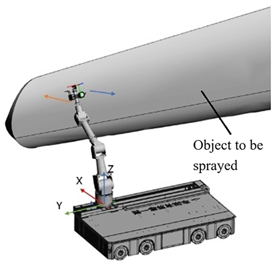
Figure 1: Schematic of the principal normal vector.

The principal spraying normal vector construction method is as follows:

1)   Determine the target spraying surface: Select the surface to be sprayed.

2)   Apply area-weighted sampling method: Generate a set of sample points {Pi} on the surface such that the local surface area represented by each point is approximately equal. This method effectively avoids overly dense sampling in small-area or high-curvature regions, ensuring the point set is uniformly distributed in the geometric sense and adequately reflects the overall shape of the surface.

3)   Calculate the normal vector for each point: For each sample point Pi, compute its unit normal vector ni.

4)   Compute the principal normal vector: Perform a vector average of all unit normal vectors, followed by normalization.

2.2.2 Conical Pose Domain

During spray painting operations, the pose at each point on a curved surface is influenced by its local curvature, meaning that a single principal spraying surface normal vector cannot satisfy the pose constraints for all trajectory points. To address this issue, the concept of a conical pose domain is introduced based on the principle illustrated in Fig. 2. Conical pose domain refers to the three-dimensional spatial region formed during the spraying process, where the spraying tool (such as a spray gun) is allowed to rotate around the principle normal vector of the spraying surface within a certain angular range. This region is represented by a cone with the primary normal vector as its axis and an apex angle of 2θ, where θ is the deviation angle representing the maximum angle between the normal vectors of all trajectory points and the primary normal vector.

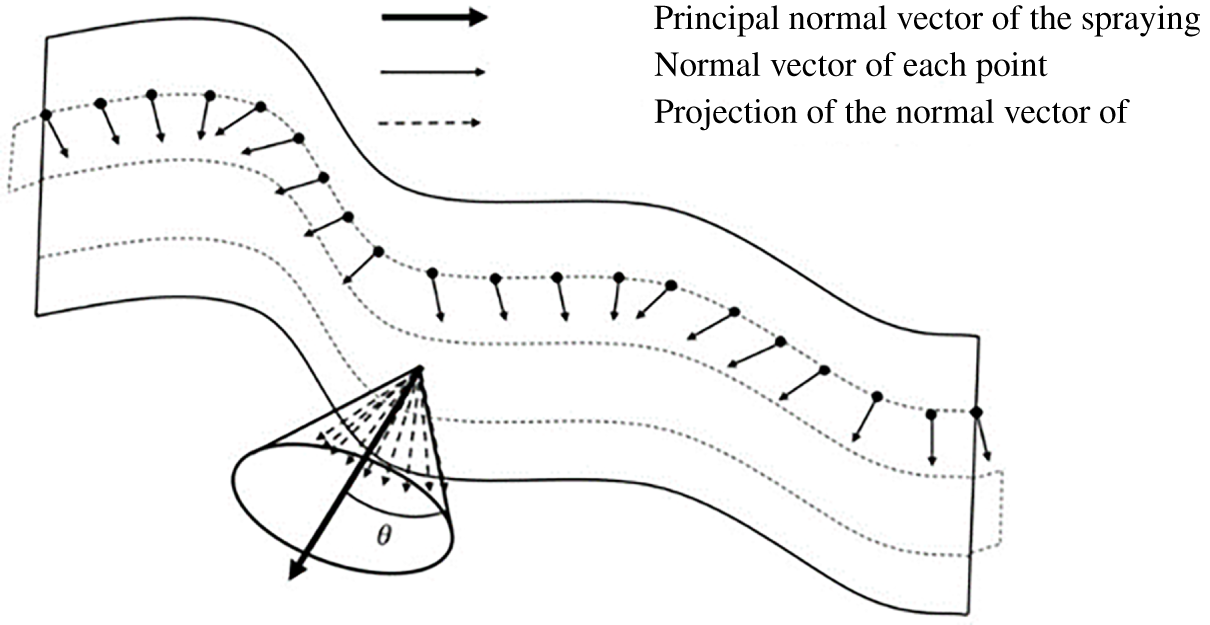
Figure 2: Schematic of the Conical Pose Domain.

Construction Steps of the Conical Pose Domain:

1)   Calculate the Point Normal Vector Deviation Angle

Traverse through all trajectory points (denoted by the black dots in Fig. 2) and calculate the angle θi between the normal vector of each point (represented by the thin solid arrow in Fig. 2) and the principal normal vector of the spraying surface (indicated by the thick solid arrow in Fig. 2).

2)   Project the Normal Vectors

Project the normal vector of each trajectory point onto the plane perpendicular to the principal spraying normal vector (the projection direction is indicated by the dashed arrow in Fig. 2).

3)   Determine the Maximum Deviation Angle

Screen all θi values from the trajectory points and take the maximum value as θmax.

4)   Construct the Pose Domain

Using the principal spraying normal vector as the axis of rotation and 2θmax as the apex angle, construct a conical space. This conical space is defined as the pose domain required for the spraying operation.

3  Calculation Method for the Workspace of Arm-Rail Coordinated Spraying Robot

3.1 Seed Space Creation

In the calculation of the workspace for an arm–rail coordinated spray painting robot, the seed space serves as the foundation for subsequent expansion. The rational selection of its center point is crucial for algorithm convergence and the quality of the final workspace. Theoretically, the center point should be located within a “pose-stable region” inside the workspace, away from joint singularities, to ensure that the end effector possesses good motion flexibility and control stability.

The steps for creating the seed space are as follows:

Step 1: First, create a robot model and calculate its reachable space using a geometric method. Take the central point of this reachable space as the center point of the seed space, denoted as (x0, y0, z0).

Step 2: Define the side lengths of the seed space: introduce parameters dwp (related to depth direction offset), wimn(minimum width), and himn (minimum height) to specify the length, width, and height of the seed space.

Step 3: Calculate the coordinate values of the eight vertices of the seed workspace.

The procedure is illustrated in Fig. 3.

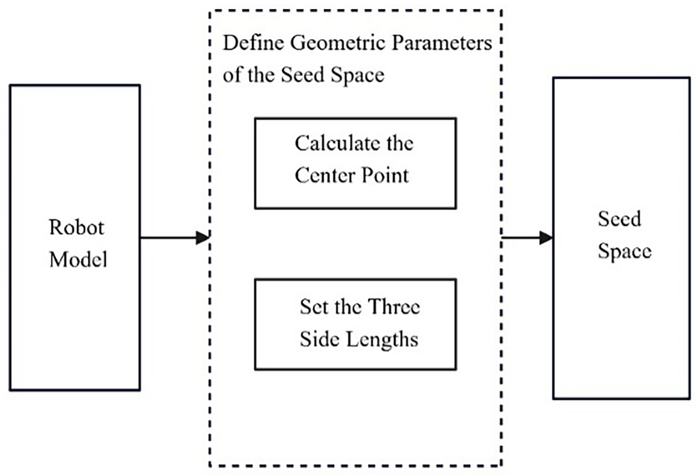
Figure 3: Flowchart of seed space creation.

3.2 Robot Workspace under Principal Normal Vector Constraints

Based on the seed space calculated in Section 3.1, an iterative process is performed along three axial directions using the principal spraying normal vector as the pose constraint, resulting in an approximate workspace for the spray-painting robot. The steps are as follows:

Step 1: Define the seed space and the principal spraying surface normal vector, and calculate the range of the seed space.

Step 2: Determine the initial width, thickness, and height of the seed workspace based on the maximum dimensions of the product to be sprayed (for the workspace of a spray painting robot, one side length of large-scale spraying surfaces is usually fixed; therefore, in this algorithm, one side length is fixed and does not participate in the iterative process. Hence, iterations are typically performed by alternating between the remaining two coordinates).

Step 3: Set the iteration step size. Use the coordinate rotation method to iteratively increment the thickness, width, and height of the seed workspace. The iteration strategy adopts a large initial step size. Each iteration requires one round of updates along all axis directions, following the order: X+, Y+, Z+, X−, Y−, Z−.

Step 4: After each increment, uniformly sample points on the surface in the direction of iteration, construct virtual spray points with the principal spraying normal vector as the pose requirement, and compute the inverse kinematic solution for these virtual spray points. If every point has a feasible inverse solution, record the length after iteration in that direction and continue iterating. If any point lacks a feasible inverse solution, record the length before iteration in that direction, reduce the iteration step size by half, and continue iterating. If the iteration step size becomes smaller than the spray spacing, record the length before iteration in that direction and stop iterating. Repeat Steps 3 and 4.

Step 5: Stop iteration in all directions and record the final lengths.

Step 6: Calculate the maximum workspace Γmn of the spray painting robot under the constraint of the principal spraying normal vector when not linked with the rail.

The specific flowchart is shown in Fig. 4.

Figure 4: Flowchart of robot workspace creation under principal normal vector constraint.

3.3 Robot Workspace under Conical Pose Domain Constraints

The approximate robot workspace Γmn obtained from Section 3.2 is further optimized by introducing the conical spraying domain as the pose constraint, resulting in the final spray painting robot workspace Γpt. The calculation method is as follows: based on Γmn computed in Section 3.2, a conical pose domain is constructed, and the seed space is reduced via the coordinate rotation method. Points are uniformly sampled on the surface of the expanded seed space, and virtual trajectory points are created with the conical pose domain as the pose requirement. During the shrinking process, points are continuously sampled and verified to determine whether the virtual trajectory points satisfy the principal normal vector pose constraint until the seed space can no longer meet this requirement. The maximum workspace recorded at that point is defined as the robot workspace under the principal normal vector constraint.

The procedure is as follows:

Step 1: Set the normal vector deviation angle according to the complexity of the surface shape of the product to be sprayed.

Step 2: Define the conical pose domain based on the normal vector deviation angle.

Step 3: Using the dimensions of Γmn as the initial values, determine the iteration step size and iteratively shrink the thickness, width, and height of Γpt using the coordinate rotation method.

Step 4: Determine the iteration step size and iteratively increase the width and height of the seed workspace using the coordinate rotation method. The strategy adopts a large step size for the first iteration, with each iteration requiring updates along all axis directions in the order: X+, Y+, Z+, X−, Y−, Z−.

Step 5: Uniformly sample points on the surface in each direction to construct virtual spray points. At each virtual spray point, establish a conical pose domain with the principal spraying normal vector as the axis. Eight generatrices are uniformly defined on the conical surface, corresponding to eight directional vectors as shown in Fig. 5.

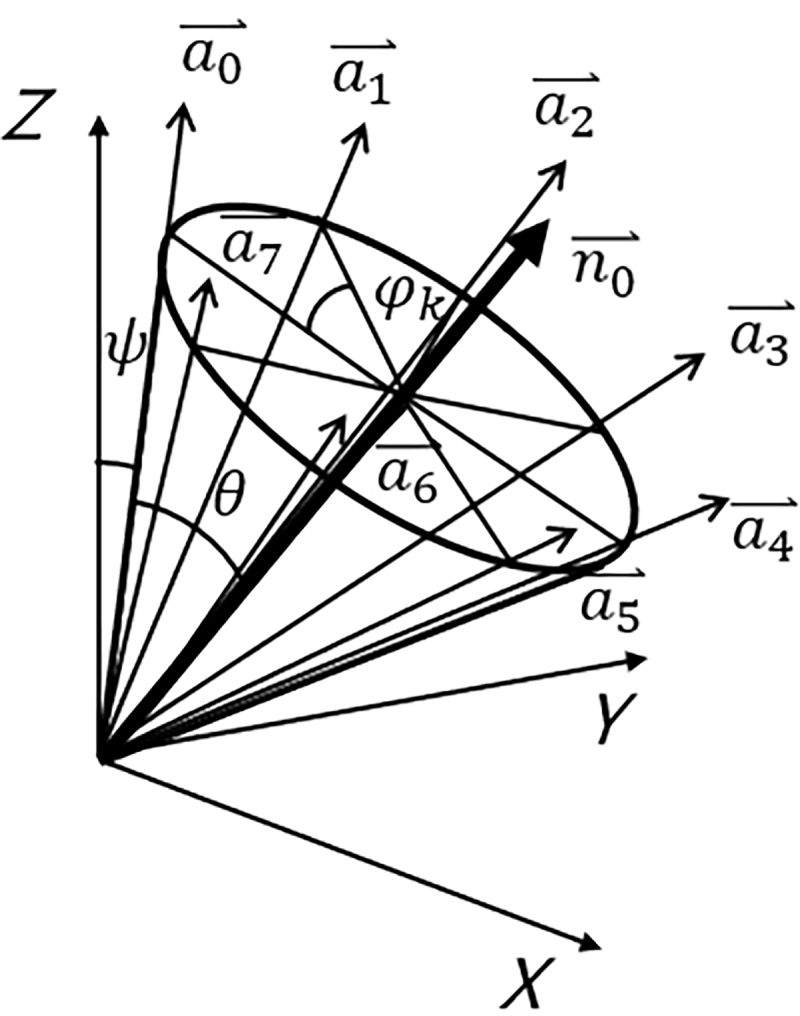
Figure 5: Schematic of generatrix direction vector construction.

Construct 8 virtual path points, and verify the spray ability of each virtual path point sequentially through inverse kinematics. If all 8 virtual path points have inverse solutions, then that virtual spray point is considered sprayable. The construction formulas are as follows:

For the j-th point Pj, with coordinates (xj, yj, zj), let the principal normal vector be denoted as n0→=[nx,ny,nz]T. Taking the point Pj as the vertex and the principal normal vector as the axis, establish a conical pose domain with an apex angle of 2θ. The initial generatrix of the cone is denoted as ξ0. Through rotational transformation, the direction vector a0→ of ξ0 can be obtained:

a0→={[nxsin⁡ψ1−nz2,nysin⁡ψ1−nz2,cos⁡ψ]T,nz≠1[sin⁡θ,0,cos⁡θ]T,nz=1(1)

where

ψ=arccos⁡(nz)−θ(2)

here, Ψ is the angle between the generatrix ξ0 and the Z-axis, located within the plane formed by n0→ and the Z-axis.

Rotating ξ0 around n0→ by an angle φk yields another generatrix ξk. Its direction vector is:

ak→=(I+n^sin⁡φk+n^2(1−cos⁡φk))a0→(3)

where I is the identity matrix, and n^ is the cross-product matrix of n0→:

n^=[0−nznynz0−nx−nynx0](4)

By sequentially taking φk = [0, π/4, π/2, 3π/4, π, 5π/4, 3π/2, 7π/4], the direction vectors (a0→, ⋯, a7→) for the 8 generatrices on the cone can be obtained.

Step 6: If every point has a feasible inverse solution, record the length after iteration in that direction and continue iterating. If any point lacks a feasible inverse solution, record the length before iteration in that direction, reduce the iteration step size by half, and continue iterating. If the iteration step size becomes smaller than the spray spacing, record the length before iteration in that direction and stop iterating and repeat Steps 4, 5, and 6.

Step 7: Continue until iteration stops in all directions, and record the final lengths.

Step 8: Calculate the maximum workspace Γpd of the spray painting robot that satisfies the normal vector deviation constraint when not linked with the rail.

The specific flowchart is shown in Fig. 6.

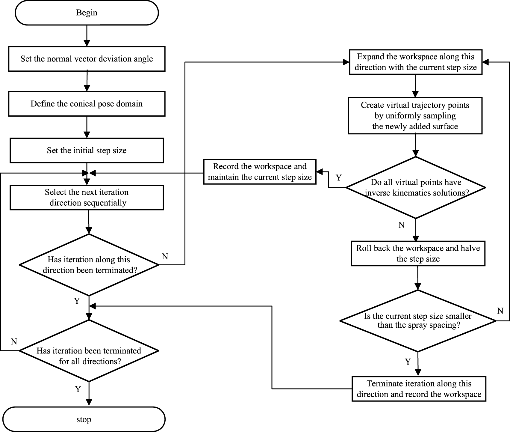
Figure 6: Flowchart of robot workspace creation under conical pose domain constraint.

3.4 Workspace of the Arm–Rail Coordinated Spray Painting Robot

Spray painting robot workspace Γpd is used to calculate the arm–rail coordinated spray painting robot workspace Γmr based on the rail speed and rail direction vector. The specific steps are as follows:

(1)   Take the center point coordinates of Γmr as (x0, y0, z0), and set the initial width, thickness, and height as the maximum width, thickness, and height (wmaxpd, wdmaxpd, hmaxpd) of the maximum workspace Γpd that satisfies the normal vector deviation constraint, obtained in Section 3.3.

(2)   Initialize the following parameters according to spray process requirements and equipment specifications:

Spraying speed Vp; Lengths of the linear rail along the X, Y, and Z axes [Lx,Ly,Lz]; Travel speeds of the linear rail along the X, Y, and Z axes [Vx,Vy,Vz].

(3)   Calculate the maximum width of the workspace Γmr when the spray painting robot is linked with the X-axis rail according to Eq. (5):

wmaxm⁢r={wmaxp⁢d+min⁡(wmaxp⁢dVp×Vx,Lx)Vx≤Vp∞Vx>Vp(5)

(4)   Calculate the maximum thickness of the workspace Γmr when the spray painting robot is linked with the Y-axis rail according to Eq. (6):

dmaxmr={dmaxpd+min(dmaxpdVp×Vy,Ly)Vy≤Vp∞Vy>Vp(6)

(5)   Calculate the maximum height of the workspace Γmr when the spray painting robot is linked with the Z-axis rail according to Eq. (7):

hmaxmr={hmaxpd+min(hmaxpdVp×Vz,Lz)Vz≤Vp∞Vz>Vp(7)

Finally, after the above three steps, an estimated size of the maximum workspace Γpd achievable when the spray painting robot is linked with the rail is obtained. Its width, thickness, and height are denoted as (wmaxmr,dmaxmr,hmaxmr).

4  Case Study: Simulation Verification

Taking the six-axis spray painting robot and AGV(automated guided vehicle) collaborative system independently developed by the research group as the test object, a simulation analysis of the arm–rail coordinated workspace calculation is performed. This system employs an AGV to carry the rail and the spray painting robot as a whole, enabling rapid adjustment of workstations. By utilizing the arm–rail coordinated motion strategy, it extends the spray coverage area and improves the efficiency and flexibility of painting large scale workpieces. The integrated system combines the mobility of the AGV, the guiding capability of the rail, and the multi degree of freedom operability of the six axis robot, allowing fast station switching and continuous spraying operations in complex working environments. Through arm–rail coordinated control, not only is the robot’s effective workspace enlarged, but also the adaptability and trajectory continuity for spraying large curved structures are enhanced. Fig. 7 shows a schematic of the spray painting robot and AGV collaboration.

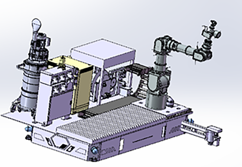
Figure 7: Schematic of the spray painting robot and AGV collaboration.

4.1 Forward Kinematics Analysis of the Spray Painting Robot

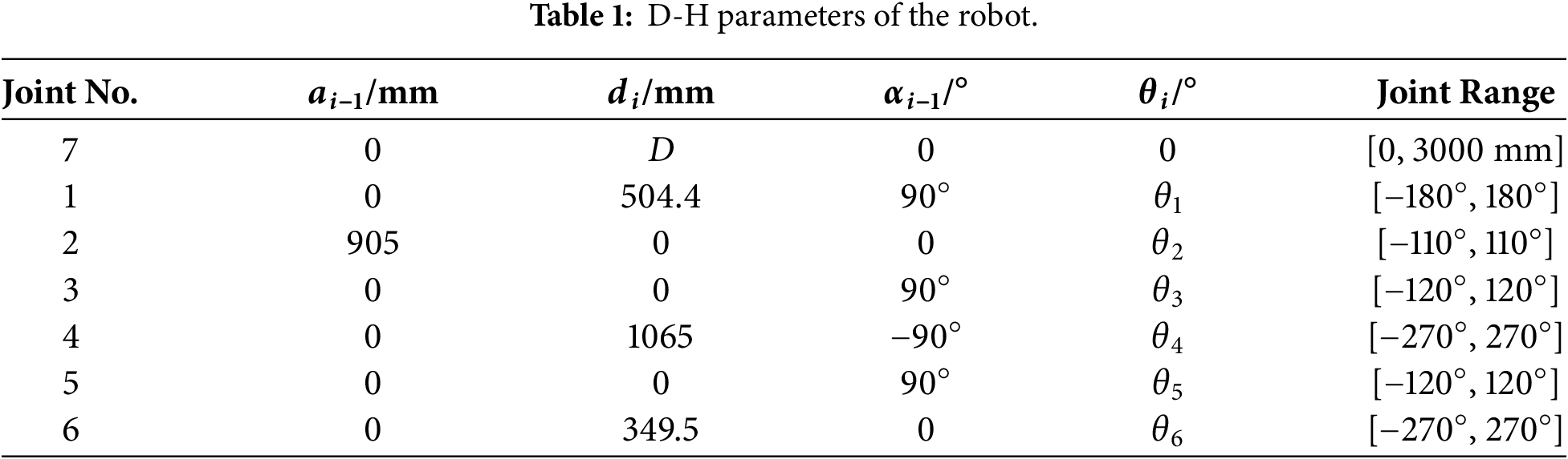
The forward kinematics of a robot refers to determining the position and orientation of the end effector relative to the base, given all joint positions and all link geometric parameters. The MD-H (modified Denavit-Hartenberg) method is used to establish the robot coordinate system, and the forward kinematics equations are derived. The corresponding D-H parameters are listed in Table 1 (Joint 7 is a prismatic joint).

The homogeneous transformation matrix between two adjacent joint coordinate systems i − 1 and i and is

Tii−1=[cθi−sθi0ai−1sθicαi−1cθicαi−1−sαi−1−disαi−1sθisαi−1cθisαi−1cαi−1dicαi−10001](8)

where: s = sin, c = cos. The forward kinematics equation of the robotic arm’s end-effector is

T60=T10⋅T21⋅T32⋅T43⋅T54⋅T65=[R1P101](9)

Finally, the transformation matrix of the end-effector is

Ttool0=10T⋅T21⋅T32⋅T43⋅T54⋅T65⋅Ttool6=[R2P201](10)

P2=[PXPYPZ]T(11)

where: R2 is the orientation matrix of the end-effector coordinate system relative to the base coordinate system; P2 is the position vector of the end-effector in the base coordinate system.

4.2 Inverse Kinematics Analysis of the Spray Painting Robot

Inverse kinematics analysis aims to determine the robot’s joint rotation angles or joint translation parameters based on the target pose of the robot’s end-effector. This problem is typically more complex than forward kinematics, primarily manifested in three aspects:

(1)   Its mathematical model is inherently nonlinear;

(2)   The solution is often non-unique;

(3)   Near singular points in the operational space, the equations may have no solution or lose valid solutions. Therefore, selecting a suitable and efficient solution method is crucial for simplifying calculations.

The solution methods for inverse kinematics can be divided into two main categories: closed-form solutions (analytical methods) and numerical solutions (iterative methods). Closed-form solutions are only applicable to specific configurations (e.g., robots satisfying the Pieper criterion). Pieper criterion states that for a six-degree-of-freedom serial manipulator, if the axes of its last three (wrist) joints either intersect at a common point or are mutually parallel, then the inverse kinematics problem of the manipulator admits a closed-form solution [19]. While numerical solutions have broader applicability. This paper adopts the Levenberg-Marquardt (L-M) numerical method to solve the inverse kinematics problem.

The core of the L-M method is to formulate the inverse kinematics problem as a nonlinear least-squares optimization problem. With the minimum pose error “e” as the optimization objective, the iterative result converges to a set of joint angles closest to the current joint angles [20]. The construction process of its objective function is as follows:

Assuming Td is the desired transformation matrix and Tc is the current transformation matrix, the pose error “e” is obtained by Eq. (12):

e(q)=‖Td−Tc‖#(12)

Since T is a complete transformation matrix, computing its norm may require more sophisticated handling—for instance, by separately calculating the norm of the position error and the norm of the rotation error, and then combining them—to obtain a scalar value representing the total pose error.

Solving the inverse kinematics is equivalent to finding a set of joint angles “q” that satisfy the following nonlinear equation:

e(q)=0(13)

Due to the existence of noise and errors, to make Eq. (13) more solvable, the L-M method replaces it with a minimization problem:

E(q)=12eTWEe→min(14)

where E(q) is a scalar objective function with respect to the system state variable q; WE denotes the weighting matrix, WE=diag{WE,i}(wE,i>0,i=1∼n(integer)). Assuming E(q) is a 6-dimensional error vector, then WE is a 6 × 6 diagonal weighting matrix, i.e., n = 6. Min indicates that the goal of this optimization problem is to minimize E(q). The objective of Eq. (14) is to find the q that minimizes E(q).

Defining the set of all possible joint configurations of the robot as Ω, inverse kinematics is the process of finding the joint angles q∈Ω that are closest to the target pose. The L-M method updates the joint angles “q” using Eqs. (15) to (17) until Eq. (14) is satisfied.

qk+1=qk+Hk−1gk(15)

Hk=JkTWEJk+WN(16)

gk=JkTWEek(17)

where k denotes the k-th iteration; Jk=J(qk) is the Jacobian matrix at joint angles qk; Hk is the coefficient matrix; gk is the gradient matrix; and WN is the damping coefficient. The damping coefficient is dynamically adjusted during the iterative process: when the damping is large, the algorithm behaves similarly to the steepest descent method, ensuring global convergence; when the damping is small, it approximates the Gauss-Newton method, achieving fast local convergence.

In the L-M method, the selection of the damping coefficient WN significantly influences the convergence performance. Introducing a biased damping coefficient effectively circumvents singularity issues and enhances the algorithm’s stability [21]. Its damping coefficient WN is defined as:

WN=λEkl+W¯N(18)

W¯N=w¯Nl(19)

where λ is a constant coefficient; Ek=E(qk), the objective value at iteration k; l is an n × n matrix, typically chosen based on the characteristic length of the links; W¯N=diag{w¯N,i}(w¯N,i>0,∀i=1∼n) are small bias values. For simplicity, W¯N is generally taken as approximately 1.0×10−3l2∼1.0×10−1l2.

4.3 Simulation Object

A wind turbine blade was selected as the coating target for verification. A schematic diagram of its dimensions is shown in Fig. 8.

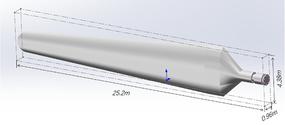
Figure 8: Schematic diagram of the basic dimensions of the wind turbine blade.

4.4 Workspace Calculation and Coating Area Division

Given the relatively small thickness of this wind turbine blade, the thickness of the workspace in the X axis direction is set to 0.96 m in this paper. Based on iterations along the Y and Z axes, the effective workspace of the painting robot is generated.

The surface to be coated is projected onto the YOZ plane along its average normal vector, resulting in a projection plane [22], as shown in Fig. 9.

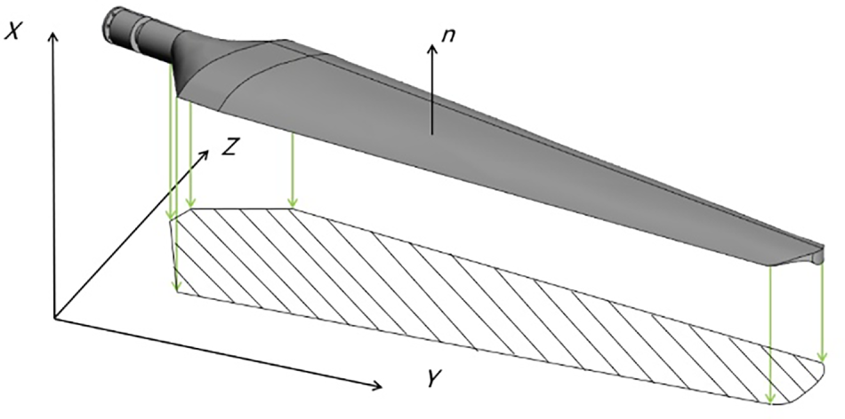
Figure 9: Generation of the 2D contour.

The figure can be discretized using a rectangular grid, as shown in Fig. 10.

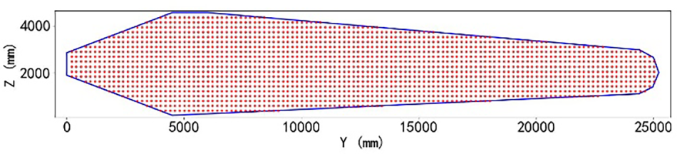
Figure 10: Schematic diagram of the point array.

The robot’s workspace is calculated to guide the division process, with all points being allocated to respective coating regions, thereby completing the coating area division. The specific calculations and area division are as follows:

(1)   Reachable Workspace Calculation and Coating Area Division

For the reachable workspace, the end-effector’s orientation constraints are not considered. Based on Sections 3.1 and 3.2, and after removing the orientation constraints, the calculated dimensions of the robot’s workspace are: X = 0.96 m, Y = 2.90 m, Z = 2.90 m, with the center point located at (0.6, 0, 0.5). Using this reachable workspace, the blade coating area is divided into 17 sections, as illustrated in Fig. 11.

(2)   Full-Orientation Workspace Calculation and Coating Area Division

Based on Sections 3.1 and 3.2, and by changing the orientation requirement to a full-orientation constraint, the calculated dimensions of the robot’s workspace are: X = 0.96 m, Y = 0.950 m, Z = 0.975 m, with the center point located at (0.6, 0, 0.5125). Using this full-orientation workspace, the blade coating area is divided into 110 sections, as shown in Fig. 12.

(3)   Conical Orientation Workspace Calculation and Coating Area Division

Considering the curved surface characteristics of the blade (with a maximum curvature of approximately 30°), the half-apex angle of the conical orientation domain is set to 30°. The workspace under the conical orientation constraint is calculated using methods from Sections 3.1, 3.2, and 3.3. The results show the workspace center point is (0.6, 0, 0.24), with dimensions of X = 0.96 m, Y = 1.42 m, and Z = 1.34 m. Based on this workspace size, the blade is divided into 59 coating areas. This method effectively reduces the number of areas while ensuring coating quality, as illustrated in Fig. 13.

(4)   Arm–rail Coordinated Conical Orientation Workspace Calculation and Coating Area Division

For the arm–rail coordinated robot, the rail speed is 100 mm/s, the painting speed is 150 mm/s, and the coordinated movement is along the Y-axis direction. Building upon the conical orientation workspace, the coordinated workspace size under arm-rail coordination is calculated to be (0.96, 4.26, 1.34) using the coordinated solution algorithm. Based on this workspace size, the blade requires only 22 coating areas, significantly improving painting efficiency, as shown in Fig. 14.

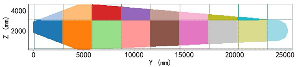
Figure 11: Reachable workspace division.

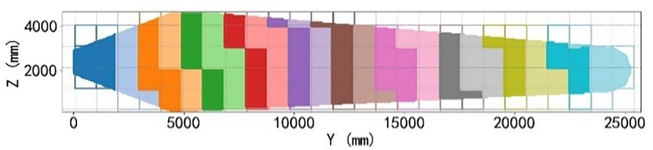
Figure 12: Full-orientation workspace division.

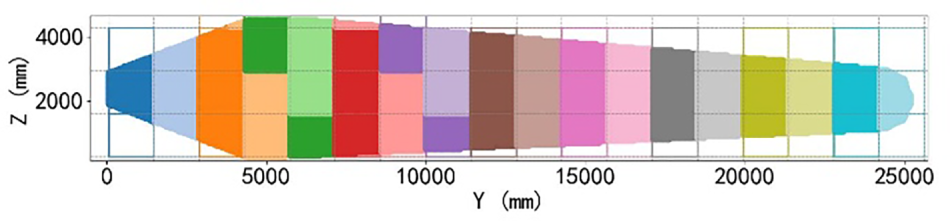
Figure 13: Conical orientation workspace division.

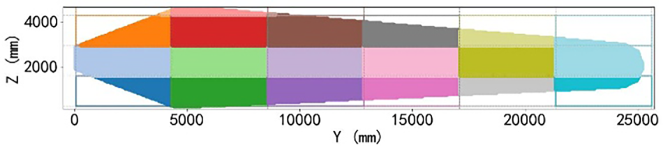
Figure 14: Coordinated workspace division for the painting robot.

4.5 Verification and Comparison

(1)   Feasibility Analysis

In the reachable workspace, some of the coating trajectory points cannot achieve an inverse kinematics solution, resulting in unreachable points during actual coating. In contrast, for the full-orientation workspace, the conical orientation workspace, and the arm–rail coordinated workspace, inverse solutions exist for all trajectory points, demonstrating good feasibility.

(2)   Coating Efficiency Comparison

The full-orientation workspace requires the highest number of coating cycles due to its strict orientation requirements and finer area division. Conversely, the arm–rail coordinated conical orientation workspace minimizes the number of areas, significantly improving coating efficiency, making it suitable for rapid coating of large-scale workpieces.

5  Conclusion

This study proposes a workspace calculation method for arm-rail coordinated spraying robot. Compared to existing methods, the novelty of the proposed approach lies in its simultaneous consideration of orientation constraints and rail speed limitations during the spraying process, thereby unifying geometric reachability and motion realizability in workspace computation. Specifically, the method incorporates a conical pose domain during the seed-expansion-based workspace generation to characterize the constraints on nozzle orientation imposed by the spraying process. Furthermore, it integrates the upper limit of rail speed to evaluate kinematic feasibility, ultimately generating a practical arm-rail coordinated workspace with meaningful spraying implications.

The results demonstrate that, compared to the traditional reachable workspace, the workspace obtained by this method exhibits higher process realizability. In contrast to the full-orientation workspace, it significantly improves spraying efficiency. Moreover, the method can directly compute the effective workspace for a single spraying pass, providing a more precise theoretical basis and operational scope for subsequent spraying task partitioning and trajectory planning.

Since the arm-rail coordinated spraying robot are still in the processing stage, the practicality and effectiveness of the proposed workspace calculation method—specifically,the extent to which it can improve efficiency, energy consumption, and spraying quality—can only be analyzed through simulations and must be verified through subsequent experiments.

Acknowledgement: Not applicable.

Funding Statement: The authors received no specific funding for this study.

Author Contributions: The authors confirm contribution to the paper as follows: Conceptualization, Kai Li and Dunmin Lu; methodology, Kai Li; software, Kai Li; validation, Kai Li, Yanbin Yao and Zhiyong Li; formal analysis, Kai Li, Yanbin Yao and Zhiyong Li; investigation, Kai Li; resources, Guolei Wang; data curation, Kai Li; writing—original draft preparation, Kai Li and Guolei Wang; writing—review and editing, Dunmin Lu, Guolei Wang, Yanbin Yao and Zhiyong Li; visualization, Kai Li; supervision, Dunmin Lu; project administration, Guolei Wang; funding acquisition, Dunmin Lu. All authors reviewed and approved the final version of the manuscript.

Availability of Data and Materials: This article does not involve data availability, and this section is not applicable.

Ethics Approval: Not applicable.

Conflicts of Interest: The authors declare no conflicts of interest.

References

1. Xu F, Zi B, Wang J, Yu Z. Multi-objective trajectory optimization for rigid-flexible coupling spray-painting robot integrated with coating process constraints. Chin J Mech Eng-En. 2024;37(1):152. doi:10.1186/s10033-024-01130-5. [Google Scholar] [CrossRef]

2. Wang Y, Xie L, Wang H, Zeng W, Ding Y, Hu T, et al. Intelligent spraying robot for building walls with mobility and perception. Automat Constr. 2022;139(2S11):104270. doi:10.1016/j.autcon.2022.104270. [Google Scholar] [CrossRef]

3. Qie J, Miao Y, Liu H, Han T, Shao Z, Duan J. Design and process planning of non-structured surface spray equipment for ultra-large spaces in ship section manufacturing. J Mar Sci Eng. 2023;11(9):1723. doi:10.3390/jmse11091723. [Google Scholar] [CrossRef]

4. Li Z, Zhao D, Zhao J. Structure synthesis and workspace analysis of a telescopic spraying robot. Mech Mach Theory. 2019;133:295–310. doi:10.1016/j.mechmachtheory.2018.11.022. [Google Scholar] [CrossRef]

5. Zheng S, Liu C, EI-Aty A, Hu S, Bai X, Sun J, et al. Design and implementation of a 6-DOF robot flexible bending system. Robot Cim-Int Manuf. 2023;84:102606. doi:10.1016/j.rcim.2023.102606. [Google Scholar] [CrossRef]

6. Zhao X, Zhao Z, Liu Y, Su C, Meng J. Analysis of workspace boundary for multi-robot coordinated lifting system with rolling base. Robotica. 2024;42(11):3657–74. doi:10.1017/S0263574724001577. [Google Scholar] [CrossRef]

7. Liu Z, Nakashima S, Komatsu R, Matsuhira N, Asama H, An Q, et al. Automatic viewpoint selection for teleoperation assistance in unmanned environments using rail-mounted observation robots. Int J Auto Tech-Jpn. 2025;19(4):554–65. doi:10.20965/ijat.2025.p0554. [Google Scholar] [CrossRef]

8. Chong Z, Xie F, Liu X, Wang J, Niu H. Design of the parallel mechanism for a hybrid mobile robot in wind turbine blades polishing. Robot Cim-Int Manuf. 2020;61(4):101857. doi:10.1016/j.rcim.2019.101857. [Google Scholar] [CrossRef]

9. Yang Z, Tian W, Wang H, Liu X, Zhang D, Yan Y, et al. Snake-like robot workspace solving method based on improved monte carlo method. Appl Bionics Biomech. 2025;2025(1):6125695. doi:10.1155/abb/6125695. [Google Scholar] [PubMed] [CrossRef]

10. Xu Y, Yang F, Mei Y, Zhang D, Zhou Y, Zhao Y. Kinematic, workspace and force analysis of a five-DOF hybrid manipulator R(2RPR)R/SP+RR. Chin J Mech Eng-En. 2022;35(5):248–59. doi:10.1186/s10033-022-00792-3. [Google Scholar] [CrossRef]

11. Chalongwongse S, Chumnanvej S, Suthakorn J. Analysis of endonasal endoscopic transsphenoidal (EET) surgery pathway and workspace for path guiding robot design. Asian J Surg. 2019;42(8):814–22. doi:10.1016/j.asjsur.2018.12.016. [Google Scholar] [PubMed] [CrossRef]

12. Zheng Q, Liu X, Yang Z, Hu X. Workspace analysis of spray painting robot with two working modes for large ship blocks in ship manufacturing. J Phys: Conf Ser. 2021;2050(1):012018. doi:10.1088/1742-6596/2050/1/012018. [Google Scholar] [CrossRef]

13. Zeng Q, Zhou G, Shi J, Li Y, Liu Y, Chen T, et al. Robot workspace optimization based on monte carlo method and multi island genetic algorithm. Mechanika. 2022;28(4):308–16. doi:10.5755/j02.mech.32035. [Google Scholar] [CrossRef]

14. He B, Zhu X, Zhang D. Boundary encryption-based monte carlo learning method for workspace modeling. J Comput Inf Sci Eng. 2020;20(3):034502. doi:10.1115/1.4046816. [Google Scholar] [CrossRef]

15. Stejskal T, Svetlík J, Ondocko S. Mapping robot singularities through the Monte Carlo method. Appl Sci. 2022;12(16):8330. doi:10.3390/app12168330. [Google Scholar] [CrossRef]

16. Chaudhury A, Ghosal A. Workspace of multifingered hands using Monte Carlo method. J Mech Robot. 2018;10(4):041003. doi:10.1115/1.4039001. [Google Scholar] [CrossRef]

17. Peidró A, Reinoso Ó, Gil A, Marín J, Payá L. An improved Monte Carlo method based on Gaussian growth to calculate the workspace of robots. Eng Appl Artif Intel. 2017;64(11):197–207. doi:10.1016/j.engappai.2017.06.009. [Google Scholar] [CrossRef]

18. Aboelnasr M, Bahaa H, Mokhiamar O. Novel use of the Monte-Carlo methods to visualize singularity configurations in serial manipulators. J Mech Eng Sci. 2021;15(2):7948–63. doi:10.15282/jmes.15.2.2021.02.0627. [Google Scholar] [CrossRef]

19. Lei M, Zhang X, Yang W, Zhang G. Inverse kinematics solution method based on workspace analysis and iterative step coefficient adjustment of general robot. Measurement. 2025;247:116807. doi:10.1016/j.measurement.2025.116807. [Google Scholar] [CrossRef]

20. Yang Q, Cui Y, Wang X. Robot inverse kinematics solving based on improved LM method. Mod Mach Tool Autom Manuf Technol. 2023;5:94–6. doi:10.13462/j.cnki.mmtamt.2023.05.022. [Google Scholar] [CrossRef]

21. Zhou P, Xu K, Wang D. Rail profile measurement based on line-structured light vision. IEEE Access. 2018;6:16423–31. doi:10.1109/ACCESS.2018.2813319. [Google Scholar] [CrossRef]

22. Lu Z, Sun L, Zhang Y. Research on path planning of curved surface spraying based on discrete points. Mech Eng Technol. 2022;11(6):621–34. doi:10.12677/MET.2022.116072. [Google Scholar] [CrossRef]