A Comprehensive Framework for Nature-Inspired Photovoltaic Model Calibration and Explainable Surrogate-Based Sensitivity Analysis

1  Introduction

Driven by the global energy transition and net-zero emission targets, photovoltaics (PV) has become a key technology for decarbonizing the power sector. The performance of PV devices is jointly determined by multiple physical and manufacturing parameters, including the photocurrent, saturation current, diode ideality factor, and the series and shunt resistances. Variations in these parameters alter the shape of the current–voltage (I–V) curve and consequently affect efficiency, process stability, and aging behavior. Because measurement and manufacturing inevitably introduce uncertainties, quantitatively under-standing the influence of each parameter is essential for model calibration, design optimization, process control, and fault diagnosis. This consideration motivates the workflow adopted in this study, where parameter identification is performed prior to sensitivity analysis.

PV cells are commonly represented by equivalent-circuit models to describe their electrical behavior with improved fidelity. Widely used formulations include the Single-Diode Model (SDM), Double-Diode Model (DDM), and Three-Diode Model (TDM), all of which consist of multiple diode branches and can effectively characterize I–V characteristics [1]. Increasing the number of diode branches may capture underlying physical mechanisms more accurately, but it also increases computational complexity. This complexity primarily arises from the larger number of unknown parameters, the implicit relationships induced by strong coupling among electrical variables, and the exponential terms in the governing equations that intensify nonlinearity. These factors make accurate modeling and numerical solving more difficult and may reduce computational efficiency.

Parameter optimization plays a crucial role in improving PV system efficiency and model reliability. Recent work [2] has pursued iteration-free yet physics-consistent evaluation of the single-diode equation for real-time emulation and controller verification. For example, Lambert-W explicit solvers were derived to avoid root-finding iterations while preserving the SDM nonlinearity, and were validated in PV emulator/MPPT testing scenarios. By identifying parameters such as reverse saturation currents, series and shunt resistances, and photo-current, the model can better reflect real device behavior and maintain stable performance under varying irradiance, load conditions, and ambient temperature [3]. However, accurate parameter extraction remains challenging. Existing approaches can be broadly categorized into conventional numerical optimization and metaheuristic optimization. Conventional numerical methods are typically deterministic and gradient-based, such as the Newton–Raphson method [4], Gauss–Seidel method [5], and the Levenberg–Marquardt algorithm [6]. Although these methods can converge rapidly near a local optimum, they are sensitive to initial conditions and may be trapped in local minima in multimodal landscapes, which is common in highly nonlinear and strongly coupled PV models. Moreover, their reliance on derivative information limits applicability to non-differentiable or discontinuous objectives. In contrast, metaheuristic methods do not require gradient information and can perform global search in complex spaces, making them more suitable for high-dimensional, nonlinear, and multimodal PV parameter estimation problems. In recent years, a substantial body of research has applied various metaheuristic algorithms to photovoltaic (PV) cell model parameter identification. Representative approaches include the genetic algorithm (GA) [7], particle swarm optimization (PSO) [8], whale optimization algorithm (WOA) [9], artificial bee colony (ABC) [10], honey badger algorithm (HBA) [11], puma optimizer (PO) [12] and grasshopper optimization algorithm (GOA) [13]. These methods demonstrate superior convergence stability and parameter estimation accuracy compared with conventional analytical techniques.

Sensitivity analysis (SA) is an essential tool for investigating how parameters influence PV model behavior. Early studies commonly employed the one-factor-at-a-time (OFAT) approach, where one parameter is perturbed while all others are held fixed to observe the output response. Although OFAT is intuitive, it cannot capture parameter interactions and is most informative only under near-linear conditions [14]. To better handle nonlinearity and multi-parameter interactions, the Morris method has been widely adopted as a low-cost screening technique for global sensitivity analysis [15], providing useful indications of nonlinear or interaction effects with relatively limited computational effort. However, Morris primarily yields relative rankings and coarse interaction clues, and it does not quantify interaction contributions explicitly. Consequently, more advanced studies have used Sobol variance decomposition [16], which partitions output variance into main and interaction effects to quantify the contribution of each parameter and provide a more complete global picture.

Despite their value, conventional SA methods remain limited in efficiency and accuracy when ap-plied to PV models that are typically high-dimensional, strongly interactive, and highly nonlinear. Moreover, existing literature that directly addresses high-dimensional nonlinear interactions among PV device-level physical parameters is still relatively scarce. To overcome these limitations, this study develops an integrated framework that couples PV parameter identification with global sensitivity analysis by combining calibration, surrogate modeling, and multi-indicator sensitivity evaluation. Specifically, core parameters of the Single Diode Model (SDM) and Double Diode Model (DDM) are first identified using an optimization-based calibration procedure, and global SA is subsequently performed using a surrogate model, thereby reducing the computational burden associated with conventional SA and im-proving practical feasibility. However, two practical gaps remain. First, calibration and sensitivity analysis are often treated as separate steps, so sensitivity conclusions may not be consistent with a well-calibrated and physically plausible parameter neighborhood. Second, variance-based SA in strongly coupled SDM/DDM settings is computationally intensive and provides limited interpretability regarding effect direction and operating-point dependence, which motivates an integrated and explainable workflow.

In this work, Random Forest (RF) [17] is adopted as a surrogate model for PV behavior because it can capture complex nonlinearities and interaction effects with strong robustness, while substantially reducing the computational cost within a physically plausible parameter neighborhood. Building on the tree-based structure, Shapley Additive Explanations (SHAP) [18] are further incorporated, together with permutation importance and bootstrap confidence intervals, to provide more robust neighborhood-based sensitivity indicators. This design addresses key limitations of OFAT, Morris, and Sobol methods in terms of interaction interpretation, effect directionality, and uncertainty quantification. Overall, the proposed SHAP-driven global sensitivity analysis for multi-parameter SDM and DDM reveals marginal effects and interaction couplings around the calibrated optimum, offering quantitative insights that can support PV design, process control, and aging diagnostics. Recent studies [19] have also explored physics-informed surrogate modeling for PV performance prediction across irradiance–temperature conditions. For example, PILoN develops a physics-informed logistic nonlinear surrogate by constructing compact proxy formulations for key points (e.g., Voc and Isc) and using bounded logistic mappings to preserve physical limits and irradiance–temperature coupling. While PILoN mainly targets module-level performance modeling and generalization over wide operating ranges, this study focuses on equivalent-circuit calibration (SDM/DDM) and sensitivity interpretation. Accordingly, the RF surrogate here is used as a fast local approximator around the calibrated optimum to enable efficient SHAP/MDI/OFAT-based sensitivity analysis, rather than full-range performance forecasting.

This study investigates five parameters in the single-diode model (SDM) and seven parameters in the double-diode model (DDM) [20], and employs a Random Forest as a surrogate of the PV physical model to improve analysis efficiency. We perform systematic sampling within a physically feasible parameter domain and compute the corresponding currents using the PV model to construct the training dataset, enabling the surrogate to learn the mapping between parameters and output current. While preserving physical consistency, this approach substantially reduces the computational burden of global sensitivity analysis, allowing SHAP to be used to interpret marginal contributions, effect directions, and interactions among parameters.

Existing PV sensitivity studies largely focus on system-level energy yield or power prediction, whereas studies that handle high-dimensionality, nonlinearity, and interactions at the device-parameter level remain relatively limited. To address this gap, we propose a surrogate-based sensitivity analysis framework that integrates Random Forest and SHAP, offering both efficiency and interpretability. The framework complements prior work under multi-parameter interaction settings and provides quantitative evidence for understanding parameter mechanisms.

Traditional sensitivity analysis methods include one-factor-at-a-time (OFAT), Morris, and Sobol. Among them, OFAT perturbs one parameter at a time while fixing the others at baseline values to quantify each parameter’s influence on the model output and identify key input factors. Its sensitivity can be expressed as:

Δi=yimax−yiminximax−ximin(1)

here, ximax and ximin denote the upper and lower bounds of the parameter xi, respectively. Likewise, yimax and yimin represent the model outputs obtained by setting xi to ximax and xi to ximin, respectively, while keeping all other parameters fixed at their baseline values. The normalized sensitivity Δi is defined as the resulting increment in the target variable Y corresponding to a standardized change in the range of the feature xi.

However, the one-factor-at-a-time (OFAT) approach is limited to local perturbations and cannot capture interactions among input factors. In highly nonlinear models, one-factor-at-a-time (OFAT) analyses are inherently local around the chosen baseline and cannot account for interactions, making them inadequate for deriving a representative global ranking of parameter influence [21]. As model complexity increases, OFAT is commonly combined with the Morris method, which serves as a low-cost screening tool for global sensitivity analysis and can reveal signals of nonlinearity or interactions. The Morris method is a sampling-based global sensitivity approach. By computing elementary effects along multiple random trajectories, it can rapidly identify influential parameters under a limited number of model evaluations and provide a preliminary indication of interaction effects [22].

In contrast, Sobol-based global sensitivity analysis decomposes the output variance into variance shares attributable to individual input parameters and their higher-order interactions. However, Sobol analysis is computationally expensive, and the required sample size increases rapidly in high-dimensional settings, which often becomes a practical bottleneck for PV problems involving many parameters and strong interactions.

With improved data availability and computing resources, machine learning (ML) has increasingly been adopted as an auxiliary tool for PV modeling and sensitivity analysis, particularly in scenarios characterized by nonlinearity, high dimensionality, and pronounced interaction effects. Prior studies report that ensemble methods such as RF have been widely applied to solar irradiance forecasting, current–voltage (I–V) curve modeling, fault diagnosis, and module health assessment.

From an interpretability perspective, Mean Decrease in Impurity (MDI) can serve as a built-in feature-importance measure in RF to provide a global ranking, but it may be biased by feature scaling and multicollinearity. By contrast, SHAP [18], grounded in cooperative game theory, decomposes an individual prediction into a baseline value plus additive feature contributions, while also providing directionality, local consistency, and interaction-related cues. This makes it better suited to capture the nonlinear coupling and operating-point dependence commonly observed in PV models. Consequently, surrogate-based SHAP analysis has emerged as an effective approach for sensitivity assessment of high-dimensional nonlinear models, preserving interpretability while reducing the heavy repeated-evaluation cost required by traditional Sobol or Morris analyses.

Although ML, surrogate modeling, and SHAP have been widely adopted across many fields, existing PV studies remain largely focused on system-level outputs such as power or energy prediction, and ML-based sensitivity analyses often emphasize environmental variables such as irradiance and temperature. In comparison, sensitivity analyses at the device-parameter level, including parameters such as photocurrent, saturation currents, diode ideality factors, and series and shunt resistances, remain relatively scarce. This gap is more pronounced for multi-parameter, strongly coupled, and highly nonlinear equivalent-circuit models such as the SDM and DDM, where an integrated framework that combines surrogate modeling, global sensitivity analysis, and interpretable explanations is still lacking. Moreover, parameter calibration and sensitivity analysis are often treated as separate steps, making it difficult to ensure that sensitivity conclusions are drawn within a physically consistent and well-calibrated parameter neighborhood. To address these limitations, this study integrates parameter identification, RF-based surrogate modeling, and SHAP-based interpretation to establish a sensitivity analysis workflow capable of handling multi-parameter nonlinearity, providing effect directionality, and revealing interaction couplings, thereby overcoming the limitations of conventional sensitivity analysis in efficiency, resolution, and interpretability.

2  Methodology

Photovoltaic (PV) physical models often involve high-dimensional and strongly coupled parameters, making conventional sensitivity analysis computationally expensive and limited in characterizing interaction effects. To address these issues, this study proposes an integrated framework that links parameter identification and sensitivity analysis in a single workflow, ensuring that sensitivity conclusions are drawn from a calibrated physical model and remain within a physically plausible and engineering-relevant parameter space.

First, parameter identification is conducted for the Single-Diode Model and the Double-Diode Model using measured V–I data. To effectively address the multimodal and nonlinear characteristics of the parameter extraction problem, the Starfish Optimization Algorithm is employed. The algorithm demonstrates enhanced global exploration capability owing to its multiple exploration strategies, which enable adaptive modulation of search dynamics and improve the robustness of the identification process. This calibration step not only improves the reconstruction accuracy of the I–V and P–V curves, but also establishes the baseline parameters and a credible neighborhood for subsequent sensitivity analysis, thereby avoiding unrealistic parameter combinations that may arise from overly broad search domains. Second, to enable large-scale sampling and sensitivity evaluation under a controllable computational budget, a Random Forest (RF) surrogate is constructed to learn the nonlinear mapping from voltage and the parameter vector to the output current. Once trained, the surrogate can be evaluated repeatedly within the physically plausible neighborhood, substantially reducing the time required by repeated solutions of the PV governing equations. Finally, SHAP are adopted as the primary sensitivity indicator to provide interpretable importance ranking and effect direction. In addition, SHAP enables sample-level analysis that reveals nonlinear and condition-dependent behaviors, complementing variance-based methods that are less informative in terms of directionality and local interaction patterns. The overall workflow is illustrated in Fig. 1.

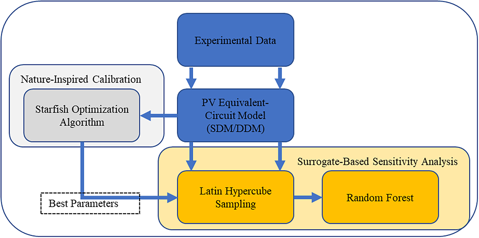
Figure 1: Overall workflow.

2.1 Photovoltaic Model

A suitable mathematical model is required to analyze the output characteristics of photovoltaic systems. A PV cell can be regarded as a diode-like device with photo response. This study considers two equivalent circuit models, namely the SDM and the DDM [20]. The following subsections present the governing equations and define the objective function used for parameter identification, which serves as the theoretical basis for subsequent calibration and characterization.

2.1.1 Single Diode Model

The SDM is one of the most widely used representations in PV studies. It describes the dominant electrical behavior of a PV cell in a relatively compact form while accounting for current losses induced by material defects and non-ideal effects, leading to predictions that better reflect practical operation. The output current IL is computed using Eq. (2).

IL=Iph−ID1−Ish(2)

ID=Isd1[exp⁡(q(VL+ILRS)n1kT)−1](3)

Ish=VL+ILRSRsh(4)

In the SDM, Iph denotes the photocurrent, ID is the diode current, and Ish is the current through the shunt branch. The diode current ID follows the Shockley diode equation, as given in Eq. (3), and the shunt current Ish is expressed in Eq. (4). Here, Isd1 is the reverse saturation current, q is the elementary charge (1.608×10−19 C). VL is the terminal voltage, and IL is the output current. The series resistance Rs represents the equivalent resistance introduced by electrodes and interconnections, while the ideality factor n1 characterizes the deviation from an ideal diode. The Boltzmann constant is denoted by k (1.6×10−23 J/K). T is the absolute cell temperature, and Rsh models leakage paths inside the cell. The parameters to be identified in the SDM are [Iph, Isd1, Rs, Rsh, n1]. Fig. 2 illustrates the SDM equivalent circuit.

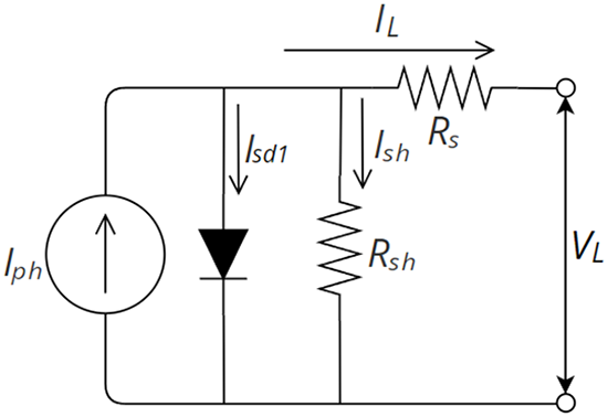
Figure 2: SDM equivalent circuit diagram.

2.1.2 Double Diode Model

Compared with the SDM, the DDM introduces an additional branch in parallel with the diode to represent extra current loss induced by recombination mechanisms. It becomes more pronounced under low-irradiance conditions. Although the DDM has a more complex structure, it typically provides higher modeling accuracy. The output current of the DDM is given in Eq. (5).

IL=Iph−ID1−ID2−Ish(5)

ID1=Isd1[exp⁡(q(VL+ILRS)n1kT)−1](6)

ID2=Isd2[exp⁡(q(VL+ILRS)n2kT)−1](7)

Isd1 and Isd2 denote the reverse saturation currents associated with diffusion and recombination effects in the two diode branches, respectively, while n1 and n2 characterize the corresponding ideality levels of these mechanisms. The parameters to be identified in the DDM are [Iph, Rs, Rsh, Isd1, Isd2, n1, n2]. The equivalent circuit is shown in Fig. 3.

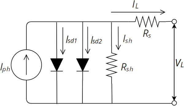
Figure 3: DDM equivalent circuit diagram.

In practical PV engineering, equivalent-circuit models such as the SDM and DDM are widely used for module characterization and model-based diagnostics. In PV system design, calibrated parameters support performance prediction under varying irradiance and temperature and are commonly embedded in simulation workflows for energy-yield estimation and operating-point analysis. In diagnostics, parameter deviations from baseline are often interpreted as fault or degradation signatures. For example, an increase in series resistance is linked to contact or interconnect degradation, a decrease in shunt resistance suggests leakage paths, and changes in diode-branch parameters can indicate recombination-related effects that are more pronounced under low-irradiance conditions. These practical roles motivate our focus on accurate calibration and interpretable parameter influence for both SDM and DDM.

2.2 Nature-Inspired Calibration: Starfish Optimization Algorithm

Metaheuristic algorithms are often inspired by biological behaviors in nature and design search mechanisms by mimicking actions such as foraging and predation. They typically involve two stages, exploration and exploitation. This study adopts the SFOA proposed by Changting Zhong et al. [23]. In SFOA, the exploration stage simulates the foraging behavior of starfish, while the exploitation stage combines predation and regeneration strategies to refine candidate solutions. The exploration mechanism employs a hybrid search scheme and selects different position-update equations according to the problem dimensionality. During exploitation, a bidirectional search guides the population toward better solutions, and the regeneration strategy is triggered by the worst-performing individual to reduce the risk of being trapped in local optima. The overall procedure is illustrated in Fig. 4.

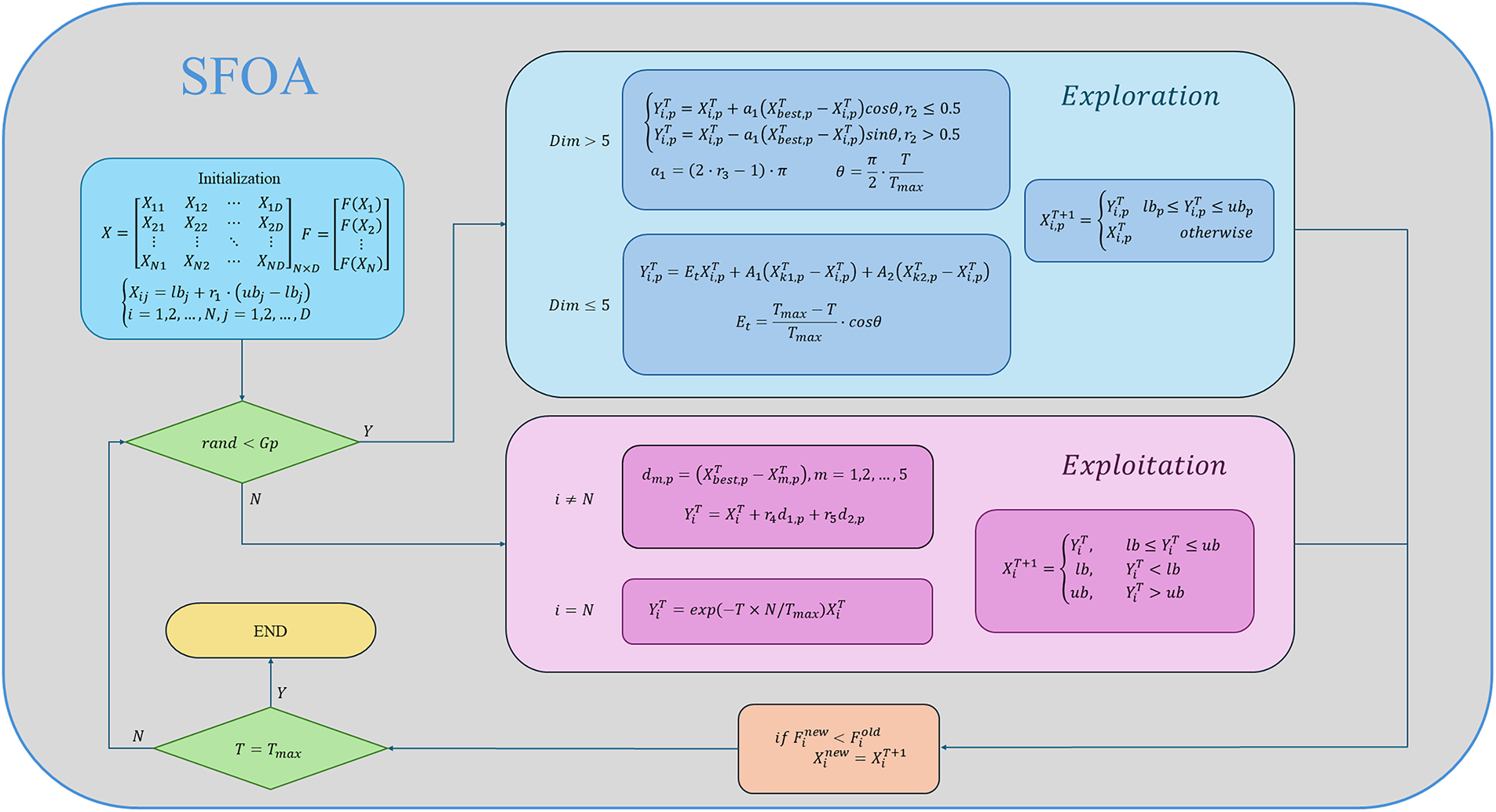
Figure 4: SFOA flow chart.

2.2.1 Initialization

At the beginning of the algorithm, the starfish population is initialized. The initialization matrix is given in Eq. (8).

X=[X11X12⋯X1DX21X22⋯X2D  ⋮  ⋮  ⋱  ⋮XN1XN2⋯XND]N×D(8)

F=[F(X1)F(X2)    ⋮F(XN)](9)

{Xij=lbj+r1⋅(ubj−lbj)i=1,2,…,N,j=1,2,…,D(10)

In Eq. (8), X denotes the starfish population, N is the population size, and D is the problem dimensionality. The initial position of each individual is generated by Eq. (10), where ub and lb are the upper and lower bounds, and r1 is a random number in (0, 1). This formulation produces N candidate individuals within the prescribed bounds. Subsequently, F in Eq. (9) stores the fitness values and is updated throughout the iterations to record newly obtained fitness values.

2.2.2 Exploration Phase

The exploration phase simulates the foraging behavior of starfish within a local region. In SFOA, five arms represent different search directions, and a hybrid strategy is employed by combining multidimensional and one-dimensional searches. When the problem dimensionality D > 5, the search space becomes large, and multidimensional updates are used to broaden exploration. When D ≤ 5, one-dimensional updates are applied to perform a more focused and efficient exploration.

{Yi,pT=Xi,pT+a1(Xbest,pT−Xi,pT)cos⁡θ,r2≤0.5Yi,pT=Xi,pT−a1(Xbest,pT−Xi,pT)sin⁡θ,r2>0.5(11)

In Eq. (11), Yi,pT denotes the updated position, Xi,pT is the current position of the i-th starfish, and Xbest,pT represents the current best position in the p-th dimension. Here, p refers to five dimensions randomly selected from the D-dimensional search space. The parameters α1 and θ are computed according to Eqs. (12) and (13), respectively.

a1=(2⋅r3−1)⋅π(12)

θ=π2⋅TTmax(13)

In Eq. (13), T denotes the current iteration and Tmax is the maximum number of iterations. The sine and cosine terms describe arm oscillations to the left or right, providing an approximately symmetric mechanism for adjusting the search direction toward the food source. The parameter α1 is randomly generated for each search agent at each iteration, r3 is a random number in (0, 1), and θ varies with the iteration index. Together, these parameters regulate the influence of the distance between the current position and the best position during the update.

When the optimization problem has dimensionality lower than 5, SFOA switches to a simpler one-dimensional search in the exploration phase. Specifically, two individuals are randomly selected from the population, and their information along the p-th dimension is used to update the position by moving along a single dimension. In Eq. (14), Xk1,pT and Xk2,pT represent the p-th dimension positions of the two selected individuals, and A1 and A2 are random numbers in [−1, 1] that control the update magnitude. The starfish energy Et is computed by Eq. (15), and the one-dimensional update rule is given in Eq. (14).

Yi,pT=EtXi,pT+A1(Xk1,pT−Xi,pT)+A2(Xk2,pT−Xi,pT)(14)

Et=Tmax−TTmax⋅cos⁡θ(15)

Xi,pT+1={Yi,pTlbp≤Yi,pT≤ubpXi,pTotherwise(16)

The starfish energy Et is computed by Eq. (15), where θ is obtained from Eq. (13). The value of Et decreases as the iteration proceeds. After the position update in the exploration phase, SFOA applies Eq. (16) to verify whether the new position violates the variable bounds, where ubp and lbp are the upper and lower bounds of the p-th dimension. The updated position is accepted if it remains within the bounds, otherwise the original position is retained to preserve feasibility.

2.2.3 Exploitation Phase

In SFOA, predation and regeneration behaviors are incorporated into the exploitation phase, and two corresponding strategies are adopted. The exploitation phase uses a parallel bidirectional search mechanism that leverages both the current best solution and the positional information of other individuals. Specifically, distances between the best individual and a set of individuals are computed, two directions are then randomly selected from this distance set, and the selected directional information is used to update each starfish position to accelerate convergence toward improved solutions.

dm,p=(Xbest,pT−Xm,pT),m=1,2,…,5(17)

dm,p denotes the distance between the global best solution and the five randomly selected starfish individuals, and Xm,pT represents the positions of these individuals along the p-th dimension. The position update rule under the predation strategy is given in Eq. (18).

YiT=XiT+r4d1,p+r5d2,p(18)

In Eq. (18), r4 and r5 are random numbers in (0, 1), and d1,p and d2,p are two distances randomly selected from the five candidates. Under the parallel bidirectional search mechanism, some candidates move toward the current best solution, while others may move away from it within the same iteration, which helps maintain population diversity and reduces the risk of premature convergence to local optima.

In nature, starfish move slowly and may be vulnerable during predation, and they can detach an arm to escape and later regenerate it. SFOA abstracts this behavior as a regeneration strategy, which is executed only by the last individual in the population, corresponding to i = N in Fig. 4. Since regeneration takes time, the algorithm mimics this period by reducing the movement speed, allowing the individual to update its position with a smaller and more conservative step size. The regeneration update rule is given in Eq. (18).

YiT=exp(−T×N/Tmax)XiT(19)

XiT+1={YiT,lb≤YiT≤ublb,YiT<lbub,YiT>ub(20)

In Eq. (19), T denotes the current iteration index, Tmax is the maximum number of iterations, and N represents the population size. If the updated position obtained in the exploitation phase exceeds the variable bounds, boundary handling is applied according to Eq. (20). Specifically, values above the upper bound are clipped to the upper bound, values below the lower bound are set to the lower bound, and positions within the feasible range are accepted as the new solutions.

The selection of SFOA is motivated not only by final solution accuracy but also by its robustness across repeated runs in the highly nonlinear and strongly coupled PV parameter space. The SDM and DDM involve exponential terms and implicit relationships, leading to multimodal objective landscapes with strong parameter interactions. Although some metaheuristics may converge faster in a single best run, SFOA emphasizes stable mean-case performance by balancing exploration and exploitation through its regeneration mechanism, thereby reducing premature convergence. As indicated by the convergence results, SFOA is not always the fastest in best-case convergence, but it achieves superior mean RMSE and lower variability across 30 independent runs. Under identical population and iteration settings, SFOA therefore offers a favorable trade-off between convergence speed, stability, and parameter estimation accuracy, making it suitable for robust calibration of nonlinear PV models.

2.3 Algorithm Setting and Objective Function

During parameter identification, the algorithm iteratively updates the model parameters within a predefined search space and substitutes the updated parameters into the objective function to compute the corresponding model output current. The goal is to determine an optimal parameter set that minimizes the discrepancy between the model output and the measured data. In this work, the root-mean-square error (RMSE) is adopted as the objective function to quantify the error between the experimental current and the model-predicted current, as defined in Eq. (21).

RMSE=1N∑t=1N(Ical−Iexp)2(21)

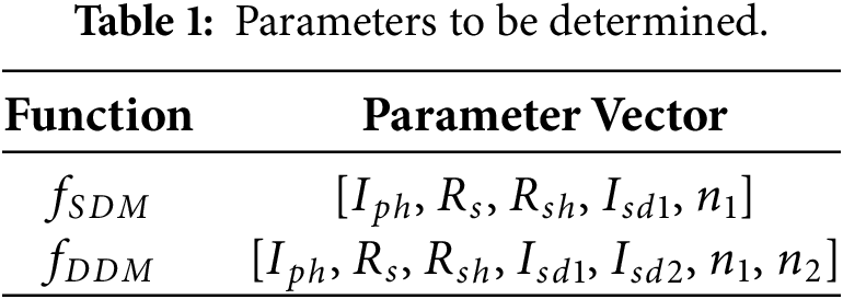
here, N denotes the number of data points, Ical is the calculated current, and Iexp is the measured current. Table 1 lists the unknown parameters to be identified for the two models.

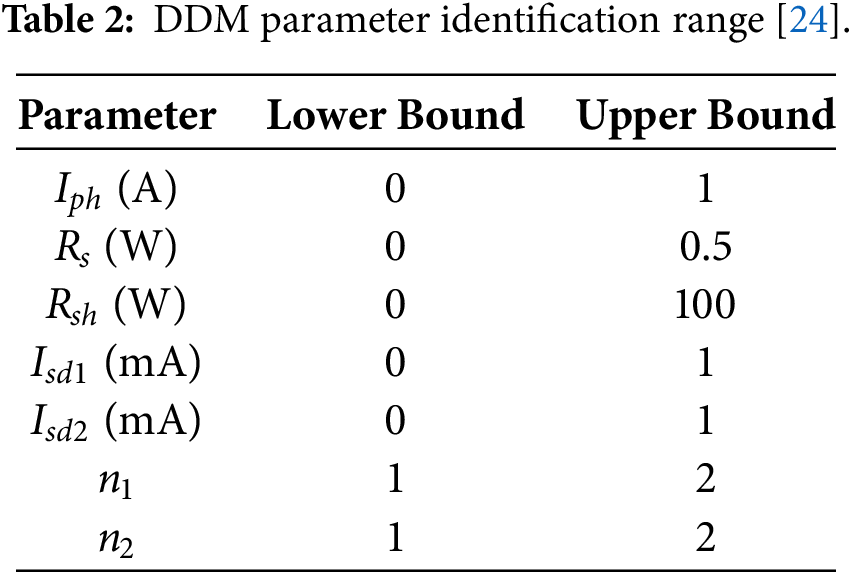
To perform PV cell parameter identification, a commercial R.T.C France photovoltaic cell is used as the test device. The measurements are conducted at an operating temperature of 303.15 K and an irradiance of 1000 W/m2, and the specifications are summarized in Table 2. Based on this dataset, SDM and DDM are employed for parameter calibration, and appropriate search ranges for the unknown parameters are set according to the literature [24], as listed in Tables 3 and 4.

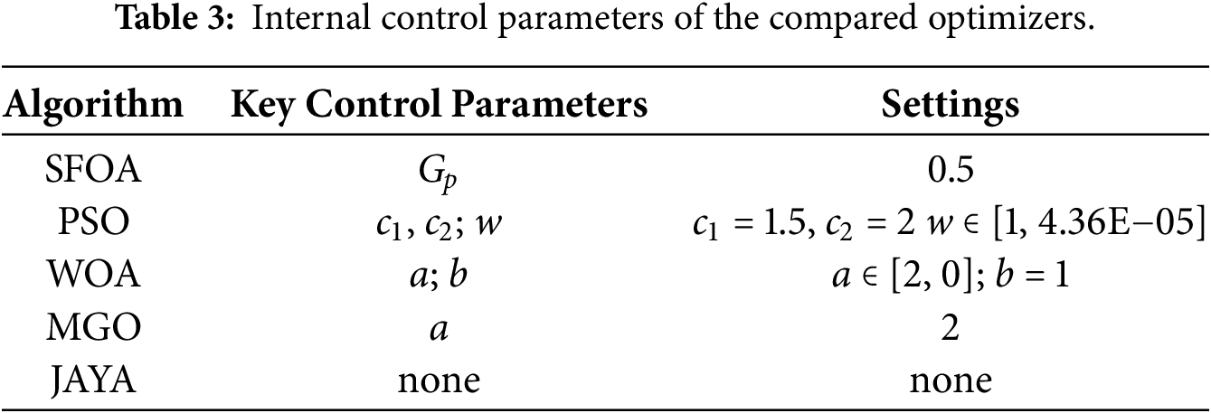
This study compares SFOA with four widely used metaheuristic algorithms for parameter identification, including particle swarm optimization, whale optimization algorithm, mountain gazelle optimizer, and the JAYA algorithm. To ensure a fair comparison and improve reliability, all algorithms are configured with the same population size, number of iterations, and control parameter settings. All implementations are conducted in MATLAB 2024a and executed on a Windows 11 Pro workstation equipped with an Intel i9-13950HX CPU and 48 GB RAM. All algorithms were implemented with a population size of 30 and a maximum of 1000 iterations, and each experiment was repeated independently 30 times to ensure statistical reliability. In this study, the Starfish Optimization Algorithm is adopted as a nature-inspired optimizer and is empirically compared with widely used metaheuristics under identical settings (population size and iteration budget), showing improved accuracy and runtime for both the Single-Diode Model and Double-Diode Model in Section 3.1. To ensure a fair comparison, all optimizers are executed under identical experimental settings in terms of population size, maximum iterations, and the number of independent runs. In addition, we explicitly report the internal control parameters of each optimizer in Table 3, following common practice in metaheuristic benchmarking.

2.4 Explainable Surrogate-Based Sensitivity Analysis

This section describes the overall workflow and methodology for sensitivity analysis. We first present the data sources and the data generation process, including measured V–I data and a large set of simulated samples generated within the feasible parameter domain using Latin Hypercube Sampling (LHS) [25]. The simulated dataset provides a more uniform coverage of the multidimensional parameter spaces of the SDM and DDM and improves the generalization of the surrogate model over the considered range.

We then describe the training procedure and parameter settings of the Random Forest model, including input features, output variables, and training strategies used to enhance stability and predictive accuracy. The RF model is treated as a surrogate that learns the input–output mapping of the PV physical model in a data-driven manner, enabling subsequent sensitivity analysis under a more tractable computational budget.

Finally, we introduce the proposed sensitivity analysis framework and explain how feature-importance measures are extracted from the RF model, including MDI and SHAP based on cooperative game theory. Multiple importance measures are used for cross-validation to improve robustness, while providing quantitative insights into effect direction, interactions, and uncertainty.

2.4.1 Sampling Strategy

For the SDM, the parameter vector is θ = [Iph, Rs, Rsh, Isd1, n1], which includes five parameters [20]. To construct a representative sample set around the calibrated solution and avoid unrealistic combinations that deviate substantially from practical behavior, sampling is conducted within a ±5 percent neighborhood of each identified optimum θi*. This setting supports surrogate model training and subsequent sensitivity analysis. The ±5 percent perturbation is designed to satisfy two requirements. It introduces sufficient variation to examine how parameters affect the output current, while preventing excessive deviation from the calibrated optimum that could cause large discrepancies between the surrogate-predicted current Irf and the physically computed current Iphys, thereby preserving physical consistency.

Within this multidimensional parameter space, LHS is used to generate 1000 parameter samples. LHS partitions the sampling interval of each parameter into N equally sized strata, and this study sets N = 1000. One value is randomly drawn from each stratum to form a length-N sample sequence for every parameter. The sampled values across parameters are then paired through random permutations to construct N non-repeated multidimensional vectors, and the samples are linearly scaled to the physical ranges of the parameters. This procedure yields 1000 parameter vectors θ(k), where k = 1, …, 1000, and each vector contains all parameters required by the PV model.

A total of 26 measured voltage–current pairs are obtained, denoted as {(Vj, Iexpj)}, j = 1, …, 26. When constructing the surrogate training dataset, these 26 measured voltages are retained as shared voltage coordinates. For each parameter vector θ(k) generated by LHS, the pair (Vj, θ(k)) is substituted into the SDM and DDM equations to compute the corresponding theoretical current. In other words, each θ(k) is evaluated at the 26 voltage points Vj, producing 26 simulated samples. Each sample uses the parameter vector θ(k) together with a voltage Vj as the input of surrogate model, and the resulting theoretical current Iphysj as the output of surrogate model. This procedure yields 26,000 simulated samples, which form the main dataset for training the Random Forest surrogate and conducting the subsequent sensitivity analysis. In this study, the 26,000 samples (26 × 1000) are used as the training set for fitting the RF surrogate. To evaluate generalization within the same near-optimum domain, an additional independent test set is generated by drawing 250 new LHS parameter vectors and evaluating them at the same 26 measured voltages, yielding 6500 test samples (26 × 250). This corresponds to an 80%–20% split between the training and test datasets. By operating within the physically plausible neighborhood of the calibrated optimum, this design provides sufficiently dense and uniform coverage in the local region, improving the stability of RF fitting and the credibility of the sensitivity outcomes. Accordingly, the subsequent sensitivity results should be interpreted as global sensitivity within this neighborhood. The surrogate accuracy reported in Section 3 is computed on this independent test set, while SHAP/MDI are derived from the RF trained on the 26,000-sample training set. We adopt a ±5% neighborhood around the calibrated solution as a physically plausible parameter domain for sensitivity evaluation. This range is consistent with the order of uncertainty commonly reported in field I–V measurements and standard correction procedures [26–28], which are typically within a few percentage points. Restricting the sampling to this interval helps avoid physically unrealistic parameter combinations while maintaining the reliability and stability of the surrogate approximation.

2.4.2 Sensitivity Analysis Based on Random Forest

After generating the LHS samples and simulated data, this study employs a Random Forest as a surrogate model to approximate the current–voltage relationship of SDM and DDM. RF is an ensemble learning method [17] and consists of multiple decision trees trained on different bootstrap subsets, which reduces the risk of overfitting in a single tree and improves stability and generalization. The final prediction is obtained by averaging the outputs of T trees. In this work, RF is not intended to replace the physical model, but to serve as a fast approximator within the feasible region constrained by the physical model and the measurements, thereby supporting the large number of repeated evaluations required by global sensitivity analysis. The SDM and DDM outputs exhibit strong nonlinearity with respect to θ and V, and the parameters are coupled through interactions. Decision trees act as piecewise models, and their ensemble can approximate complex nonlinear mappings. Therefore, RF can capture nonlinearities and interactions without increasing the structural complexity of the physical model, making it suitable as a surrogate. The LHS sampling is intentionally restricted to a ±5 percent neighborhood around the calibrated optimum so that the surrogate is only used in a physically reliable region and the risk of extrapolation to low-credibility regions is reduced. Model behavior outside this range is not included in the sensitivity conclusions of this study. In this study, SHAP-based sensitivity analysis is performed on a dataset spanning the measured I–V curve by evaluating each sampled parameter vector at all measured voltage points. This setup allows parameters to vary simultaneously, thereby reflecting interaction effects, while the Random Forest surrogate captures nonlinear and condition-dependent responses to enable efficient sensitivity evaluation. Strictly speaking, the surrogate and all reported importance rankings are valid only within a physically plausible ±5% neighborhood around the calibrated solution. Therefore, the results should be interpreted as global sensitivities conditional on this local domain.

In this study, the physically computed current Iphys is treated as the reference of RF surrogate, and the RF-predicted current Irf is evaluated by their discrepancy using the RMSE and coefficient of determination (R2) as the primary metric. The RF hyperparameters were selected through validation within the considered parameter neighborhood. For the SDM surrogate, the optimal configuration included 50 trees with a maximum depth of 30. For the DDM surrogate, 750 trees were adopted to better accommodate the higher-dimensional parameter space. In both cases, bootstrap sampling and squared-error criteria were used. The RF model is positioned as a PV surrogate operating within a ±5 percent neighborhood around the calibrated optimum, where the sample coverage is sufficiently dense and its approximation quality has been verified through error and stability checks. Under these conditions, the sensitivity results derived from RF using MDI and SHAP can be interpreted as a physically plausible approximation of SDM and DDM behavior within the considered domain, rather than purely empirical indicators from a black-box model.

2.4.3 Sensitivity Analysis Based on Feature Importance

To quantify the influence of parameters on the output current, feature-importance measures are computed after training the RF surrogate, leveraging the structure of the tree ensemble to assess each parameter contribution to the PV I–V behavior. This study adopts SHAP global importance as the primary sensitivity metric and ranks features by their mean absolute SHAP values (mean |SHAP|) across all samples [18], with MDI as a supporting indicator. In addition, OFAT is employed as a cross-check to examine effect direction and marginal trends.

SHAP originates from cooperative game theory and has been widely adopted for model interpretability to attribute the contribution of each feature to a prediction. Its key idea is to decompose the prediction for a given sample into a baseline value plus the sum of feature contributions, while satisfying additive consistency and a principled allocation of contributions. For complex models, interpretability is as important as predictive accuracy, and SHAP provides a unified explanation framework without sacrificing model performance. For a single sample, the SHAP value represents how much a feature increases or decreases the prediction, and it is defined as follows.

ϕi=∑S⊆N∖{i}|S|!(|N|−|S|−1)!|N|

here, ϕi is the SHAP value of feature i for a single sample, S denotes a feature subset that does not include i, and N is the set of all features. The terms f(S) and f(S∪{i}) represent the model prediction using only the features in S, and the prediction after adding feature i to S, respectively. This formulation computes the average marginal contribution of feature i over all possible subsets, and can be interpreted as the expected increase or decrease in the model output caused by adding feature i. To obtain a global-level importance ranking, this study adopts the mean absolute SHAP value across all samples, mean |ϕi|, as the sensitivity measure. Because the RF surrogate takes both voltage and model parameters as joint inputs, SHAP values are computed at the sample level conditional on voltage. Each SHAP attribution therefore corresponds to a specific voltage–parameter combination. The global rankings reported in this study are obtained by averaging the absolute SHAP values across all samples within the ±5% neighborhood around the calibrated optimum. Accordingly, the presented importance structure represents a voltage-aggregated global sensitivity profile over the entire I–V curve, while operating-point dependence is inherently reflected in the SHAP distributions.

In contrast, Sobol and Morris mainly provide global indices that quantify contributions to output variance, and they are less informative for explaining why a particular sample yields a higher or lower output at a specific operating point. In this study, the average effect magnitude of feature i across samples enables near-optimum global importance ranking. This is particularly useful for highly coupled PV parameters. Moreover, SHAP provides both direction and magnitude with distribution-based visualizations. Once the RF surrogate is trained, SHAP values can be computed by traversing the tree structure for additive attribution, avoiding the extensive repeated evaluations required by Sobol or Morris and offering improved efficiency and local interpretability.

Another indicator is MDI, which is a commonly used built-in feature-importance measure in RF. MDI aggregates the impurity reduction contributed by a feature over all split nodes across all trees, and the accumulated reduction is used to quantify the importance of that feature. In this study, MDI is treated as a supporting indicator to corroborate the near-optimum global importance ranking obtained from SHAP.

To validate the effect direction and marginal trends indicated by SHAP, an additional one-factor-at-a-time (OFAT) analysis is conducted for comparison. OFAT varies one parameter while keeping the others fixed, examines the resulting change in the RF-predicted current, and compares the trend with the SHAP and MDI findings to check interpretive consistency. Overall, SHAP serves as the primary sensitivity tool, and MDI together with OFAT provides cross-validation, improving the robustness and credibility of interpretations regarding importance ranking, effect direction, and parameter interactions.

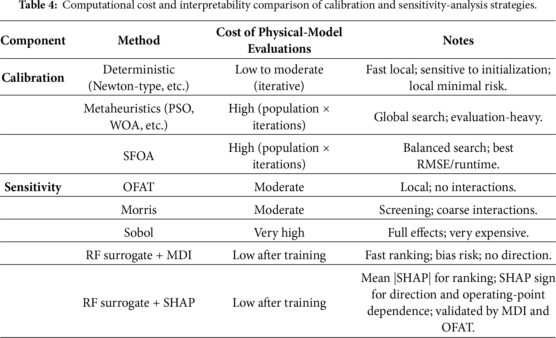
To further benchmark the proposed integrated pipeline against commonly used state-of-the-art practices, we summarize its computational complexity and interpretability in comparison with representative calibration and sensitivity-analysis strategies. For parameter identification, conventional deterministic solvers (for example, Newton-type or Levenberg–Marquardt schemes) can converge rapidly near a local optimum but often require good initialization and may be trapped in local minima for multimodal PV equivalent-circuit objectives. Metaheuristic optimizers alleviate this limitation by global exploration at the cost of iterative physical-model evaluations.

For sensitivity analysis, variance-based methods such as Sobol estimate main and interaction effects by repeated evaluations of the original physical model, which can be computationally demanding for nonlinear PV models where each evaluation involves solving implicit I–V equations across multiple operating points. Screening methods such as Morris reduce the evaluation budget but provide only coarse interaction indications, while one-factor-at-a-time analysis is intuitive yet inherently local around a baseline and cannot account for interactions. By contrast, the proposed approach shifts most computational burden to a one-time data generation and surrogate training stage. After the Random Forest surrogate is trained within a physically plausible neighborhood around the calibrated optimum, sensitivity quantification is performed efficiently on the surrogate. Shapley Additive Explanations are used as the primary measure to provide both global ranking via mean absolute SHAP values and sample-wise directional interpretation that reveals operating-point-dependent effects. Mean decrease in impurity and one-factor-at-a-time analysis are additionally used for cross-validation. Table 4 summarizes the comparison in terms of physical-model evaluation demand and interpretability features.

3  Results and Discussion

This section validates the effectiveness of the proposed integrated framework and follows the workflow order by presenting parameter identification first and sensitivity analysis second. For parameter identification, to evaluate the performance of the SFOA on the SDM and the DDM, SFOA is compared with four representative metaheuristic algorithms. Its convergence behavior is examined using both the best convergence curve and the mean convergence curve, and the results of multiple independent runs are used to compare accuracy, stability, and computational efficiency across algorithms. For sensitivity analysis, the optimal parameters obtained from the calibration stage are used as the baseline, and a Random Forest surrogate model is employed for global sensitivity evaluation within a ±5 percent neighborhood around the calibrated optimum. SHAP are adopted as the primary indicator, supported by MDI and OFAT analysis for cross-validation, to quantify the relative contributions of parameters to the output current while interpreting effect direction and condition-dependent behavior. This further verifies the consistency of the sensitivity conclusions across different indicators and their physical plausibility.

3.1 Parameter Estimation

The convergence behavior of an algorithm reflects its capability to avoid being trapped in local optima. Table 5 summarizes the identified the SDM parameter values obtained by the five algorithms, including the best value, mean value, standard deviation, and the average runtime per independent run. The results indicate that, for the SDM parameter identification, SFOA can effectively reduce computational time while achieving a superior solution. Fig. 5 illustrates the convergence behavior of SFOA and the other four algorithms for the SDM, showing that SFOA exhibits the best overall performance among the five methods. Table 6 reports the identified DDM parameter values obtained by the five algorithms, together with the best value, mean value, standard deviation, and the average runtime per independent run. These results similarly show that, for DDM parameter identification, SFOA attains better solutions while reducing the time cost. Fig. 6 presents the convergence behavior of the five algorithms for the DDM, where SFOA again demonstrates the best performance. Figs. 7 and 8 show the I–V and P–V curves of the SDM and DDM computed by SFOA, indicating an excellent agreement between the predicted curves and the experimental measurements. Moreover, the best RMSE values achieved for both the SDM and DDM are comparable to those reported in the literature under similar experimental conditions, further supporting the validity of the proposed calibration results [12].

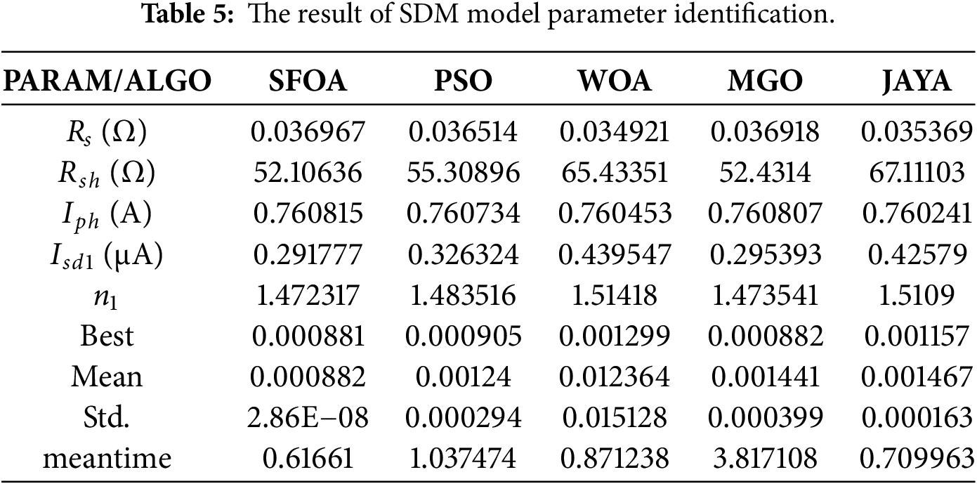
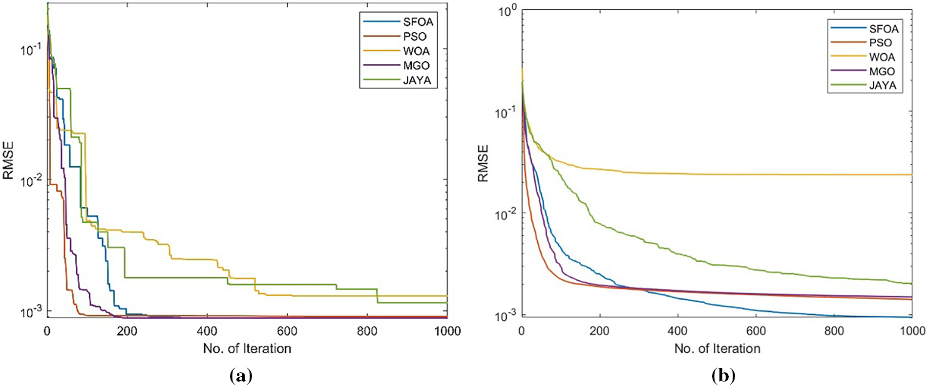
Figure 5: Convergence curves of five algorithms for searching the SDM (a) best solution and (b) mean solution.

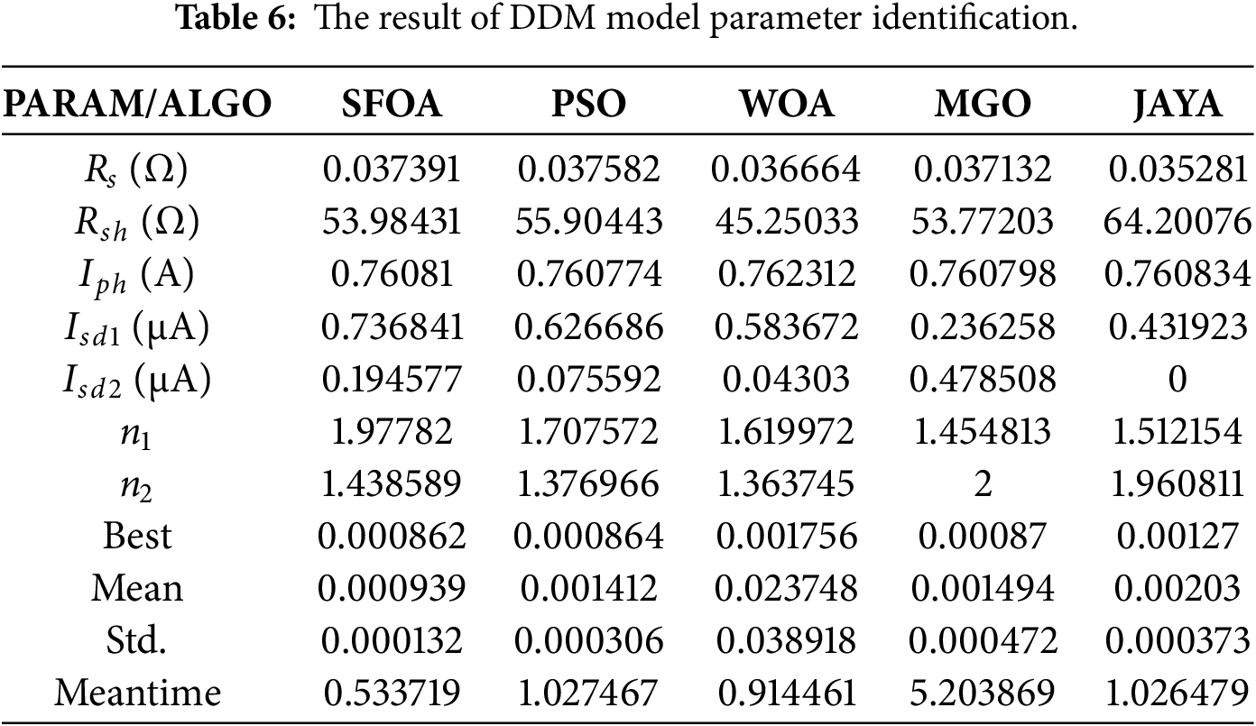
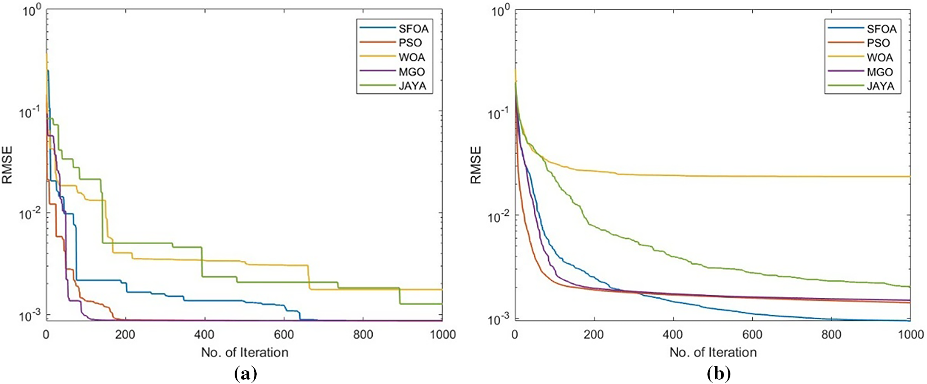
Figure 6: Convergence curves of five algorithms for searching DDM (a) best solution and (b) mean solution.

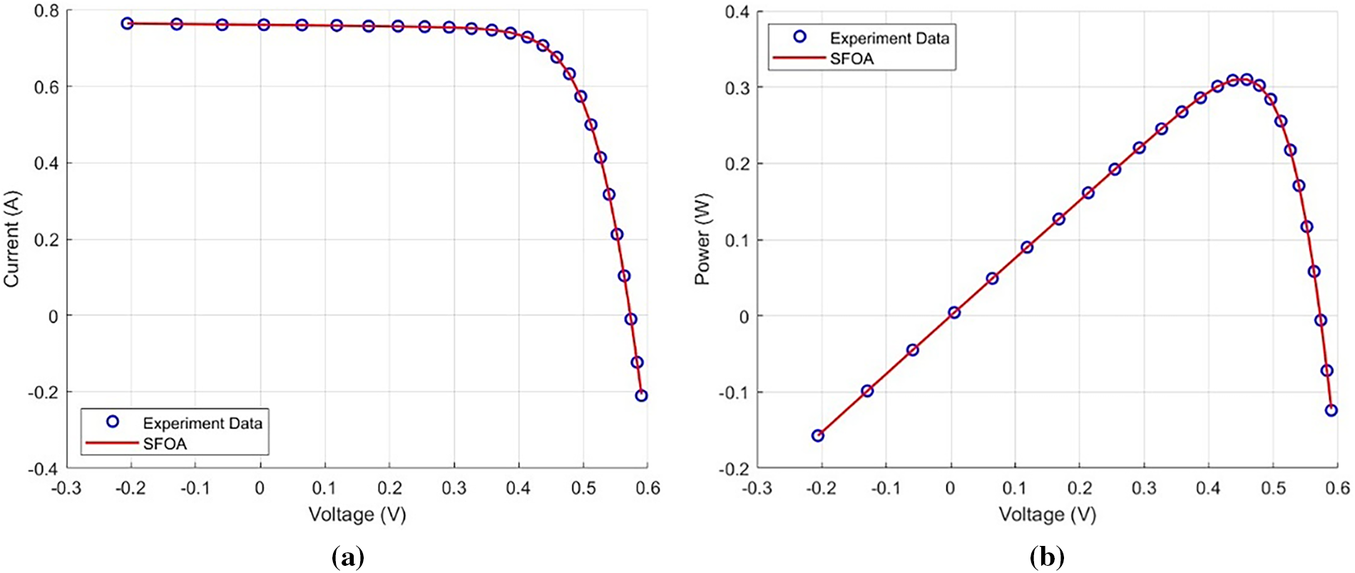
Figure 7: The comparison of experimental values of SDM with the (a) I-V and (b) P-V curves calculated by SFOA.

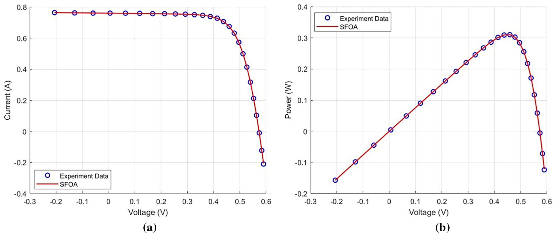
Figure 8: Comparison of the experimental values of DDM with the (a) I-V and (b) P-V curves calculated by SFOA.

Overall, the results demonstrate that SFOA achieves strong performance on both PV models, not only in parameter identification but also in predicting the I–V and P–V characteristics. Moreover, SFOA completes independent runs within a short time without compromising accuracy, suggesting high stability and further confirming its suitability for PV model calibration.

3.1.1 SDM Calibration

In the SDM parameter identification, SFOA achieves the best RMSE of 0.0008818 among all compared algorithms. In addition, SFOA requires only 0.61661 s on average, and it attains the lowest standard deviation of 2.86E−08, indicating excellent computational efficiency and strong stability. As shown in Fig. 7, the resulting I–V and P–V curves closely match the experimental data, demonstrating that SFOA can accurately identify the key SDM parameters and provide a reliable basis for subsequent analysis.

3.1.2 DDM Calibration

In DDM parameter identification, SFOA achieves the best RMSE of 0.0008811, outperforming all competing algorithms, as summarized in Table 6. In terms of computational efficiency, SFOA requires only 0.82585 s, which is substantially faster than the other methods, while its standard deviation of 2.33E−07 indicates high stability. As shown in Fig. 8, the parameters identified by SFOA yield convergence curves that closely match the experimental measurements, demonstrating strong accuracy for high-dimensional calibration tasks in photovoltaic cell models.

To statistically verify whether the observed performance differences are significant, we further conducted a nonparametric Wilcoxon rank-sum test on the results of 30 independent runs. The test indicates that SFOA achieves significantly better identification accuracy than PSO, WOA, MGO, and JAYA for both SDM and DDM (p < 0.05 in all pairwise comparisons). Moreover, the corresponding effect sizes are consistently larger than 0.5, suggesting that the improvements are not only statistically significant but also practically meaningful in magnitude.

3.2 Sensitivity Analysis

All importance rankings reported in this section are evaluated within a ±5% neighborhood around the calibrated optimum, and thus represent global sensitivity structures. On the independent test set (6500 samples), the RF surrogate achieved an RMSE of 0.001331 and R2 = 0.999366 for the SDM, and an RMSE of 0.003090 and R2 = 0.999394 for the DDM. The high R2 values and low prediction errors indicate that the RF surrogate accurately approximates the physical model within the considered neighborhood, providing a reliable basis for subsequent sensitivity analysis.

To investigate how each parameter in the equivalent-circuit PV models influences the I–V characteristics, sensitivity analysis is conducted to quantify the relative contribution of model parameters to the output current. Rather than relying on a single measure, this study adopts three sensitivity indicators, including SHAP, MDI, and OFAT, and compares their outcomes to improve the credibility and robustness of the analysis. Global sensitivity analysis is performed for both the SDM and DDM to examine whether consistent importance trends are observed across different methods. In addition, SHAP visualizations are used to further interpret local sample-level behavior, providing deeper insights into effect direction and nonlinear patterns in how parameters influence the output current. The optimal battery parameters used in this experiment are derived from the values obtained from SFOA in Tables 5 and 6.

3.2.1 Global Importance Ranking for SDM (SHAP, MDI, OFAT)

In the SDM, five parameters are considered, including the photocurrent Iph, reverse saturation current Isd1, diode ideality factor n1, series resistance Rs, and shunt resistance Rsh. Table 7 summarizes the SDM Sensitivity values under SHAP feature importance, OFAT, and MDI.

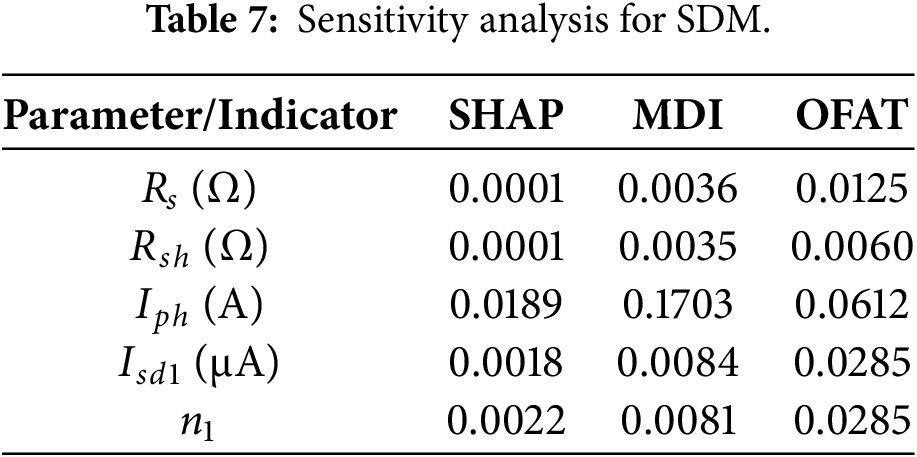
Although the three metrics in Table 7 are defined differently, they lead to highly consistent conclusions for the SDM. Using the mean absolute SHAP value (mean |SHAP|), the parameters can be categorized into three tiers by order-of-magnitude differences. Iph forms the first, dominant tier, with an importance about 8.6 times that of the next most influential parameter, n1. The second tier comprises n1 and Isd1, which have similar magnitudes and moderate effects. The third tier includes Rs and Rsh, whose importance is substantially lower, at roughly 1/18 of Isd1. MDI reflects the dependence of the random forest on each feature during node splitting, and it shows the same tiering trend. Iph remains markedly larger than the other parameters, n1 and Isd1 lie in a similar intermediate range, and Rs and Rsh again fall into the lowest tier, contributing relatively little to impurity reduction. OFAT evaluates output-current variation by perturbing one parameter while holding the others fixed, and it yields the same hierarchical structure.

Taken together, the SHAP, MDI, and OFAT results consistently indicate that Iph is the key dominant parameter governing SDM I–V behavior. n1 and Isd1 provide secondary but non-negligible influences, while Rs and Rsh play only a fine-tuning role within the “best-solution ±5%” neighborhood considered in this study. The agreement in ranking and tiering across methods not only strengthens the credibility of the sensitivity conclusions, but also supports the validity of using the RF surrogate for sensitivity evaluation. The result provides a solid basis for further SHAP-based interpretation of effect direction and condition-dependent behavior.

Fig. 9 presents the SHAP summary plot for the SDM, illustrating the distribution of SHAP values for each parameter. The horizontal axis shows the SHAP value, which indicates both the magnitude and direction of a parameter’s contribution to the model output. The vertical axis lists the parameter names. The color encodes the relative feature value in each sample, ranging from low values in blue to high values in red.

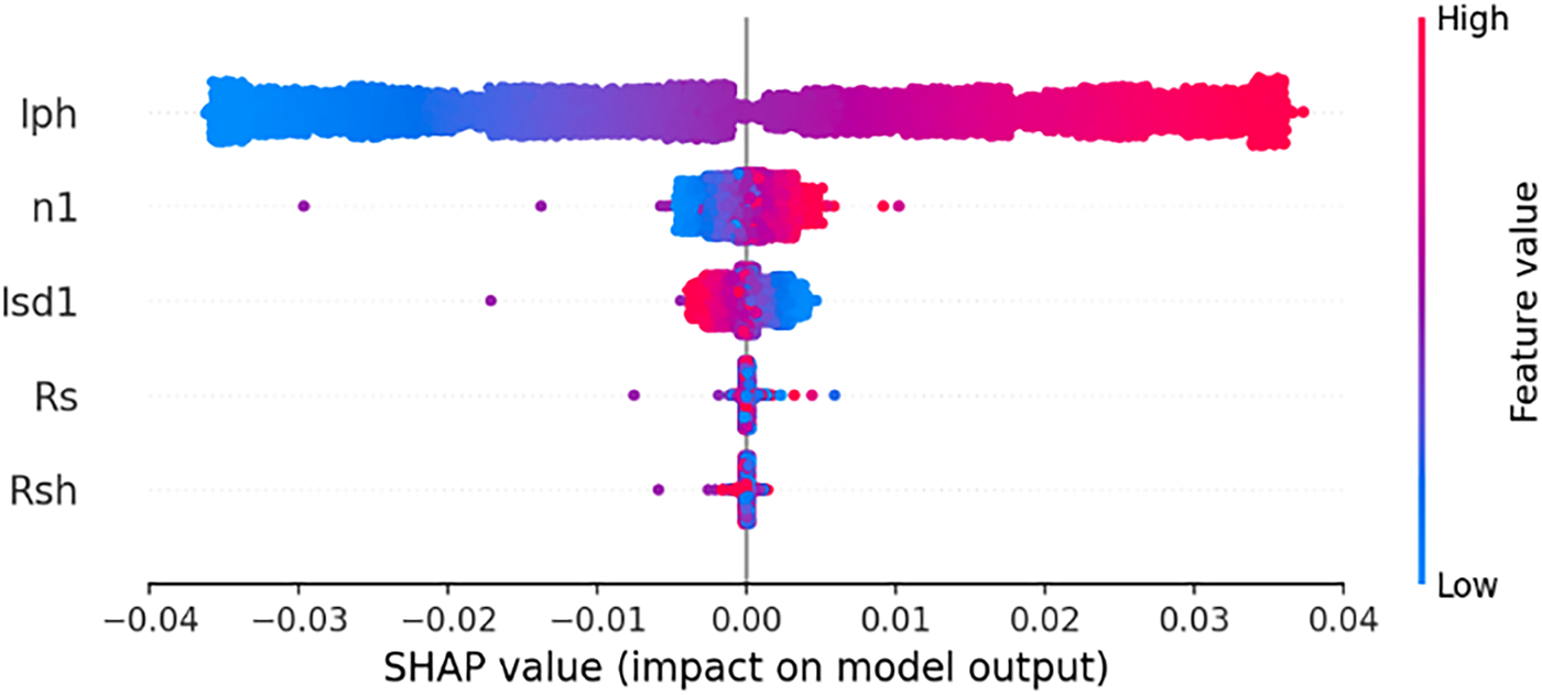
Figure 9: SHAP summary plot for the SDM.

First, Iph exhibits the widest SHAP spread, with a noticeably larger horizontal range than the other parameters, which is consistent with its highest global importance reported in the previous subsection. As shown in Fig. 9, when Iph takes larger values (red points), most samples fall in the positive SHAP region, indicating an increase in the output current. Conversely, when Iph is smaller (blue points), the points concentrate in the negative SHAP region, suggesting a reduced current.

For n1 and Isd1, although the SHAP magnitudes are clearly smaller than those of Iph, their distributions still show a non-negligible spread, indicating that the diode ideality factor and the saturation current exert secondary yet meaningful influences. Fig. 9 further shows that, for both n1 and Isd1, SHAP values associated with high and low feature values can appear on either the positive or negative side, implying nonlinear and condition-dependent effects. More specifically, for n1, larger feature values are associated with positive SHAP values for most samples, suggesting that a higher n1 tends to slightly increase the output current in many cases. An opposite tendency is observed for Isd1. Larger values of Isd1 are mostly linked to negative SHAP values, implying that an increased saturation current generally decreases the output, while a small number of samples still show positive contributions. Overall, both parameters exhibit a globally monotonic tendency toward a dominant direction, yet the same feature value may lead to opposite effects under different conditions. This behavior suggests that their influence on the output current is not purely linear, but strongly depends on the instantaneous voltage and the configuration of other parameters. In contrast, the SHAP values of Rs and Rsh are highly concentrated around zero, with only a very narrow horizontal spread, indicating that within the ±5 percent perturbation range around the calibrated optimum, their small variations contribute only marginally to changes in the output current.

Overall, the SHAP distributions shown in Fig. 9 not only quantify the magnitude and direction of each parameter’s contribution to the output current, but also provide sample-level details that conventional sensitivity measures cannot readily offer. The resulting global ranking and directional patterns are highly consistent with those from MDI and OFAT, further supporting the validity and reliability of using SHAP as the primary sensitivity tool in this study.

3.2.2 Global Importance Ranking for DDM (SHAP, MDI, OFAT)

For the DDM, seven parameters are identified, including the photocurrent Iph, the reverse saturation current of the first branch Isd1, the ideality factor n1, the reverse saturation current of the second branch Isd2, the ideality factor n2, the series resistance Rs, and the shunt resistance Rsh. Similar to the SDM analysis, the results are discussed from two perspectives, namely the global importance ranking and the SHAP distribution within a ±5 percent neighborhood around the calibrated optimum. Table 8 summarizes the Sensitivity values under SHAP feature importance, OFAT, and MDI.

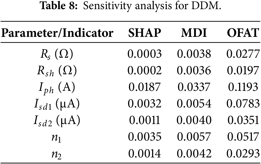
In the global sensitivity results for the DDM, the three indicators use different metrics yet reveal a highly consistent parameter-importance structure. From the SHAP results, Iph is clearly larger than the other parameters, forming the first-tier dominant factor. Its gap from the next most important parameter, Isd1, reaches 0.0152, indicating an overwhelming impact on the output current. n1 and Isd1 fall into the second tier with similar magnitudes, suggesting that the ideality factor and saturation current in the first diode branch jointly govern the major nonlinear behavior. The remaining parameters, n2, Isd2, Rs, and Rsh, show relatively low importance and belong to the third tier, mainly serving fine-scale corrections. The MDI results also rank Iph as the highest, and the gap to the next parameter Isd1 is about 0.028, exhibiting a tiering pattern in which Iph leads distinctly while the others are close in magnitude. This indicates that the random forest relies heavily on Iph when splitting nodes, whereas the other six parameters are mostly secondary, with differences primarily reflected in their ability to fine-tune prediction errors. OFAT yields the same trend. Iph remains the parameter with the largest variation effect, followed by Isd1 and n1. Although the second-branch parameters (n2, Isd2) and the resistive terms (Rs, Rsh) are smaller in effect, they still contribute to some extent, implying that the multi-branch structure and series–shunt resistances in the DDM mainly influence more subtle operating regions.

Taken together, the three analyses (SHAP, MDI, and OFAT) show that the overall ranking in the DDM follows a trend similar to that of the SDM within the examined ±5% neighborhood, Iph consistently remains the most critical dominant parameter, followed by n1 and Isd1 in the first diode branch. In contrast, the second-branch parameters (n2, Isd2) and Rs/Rsh act largely as auxiliary adjustment factors. This suggests that, even when the model is extended from the SDM to the DDM, the core sensitivity structure governing I–V behavior is still dominated by the photocurrent and the first-branch diode parameters. The added branch and resistive terms mainly compensate for finer curve shapes and local discrepancies, improving the model’s descriptive capability in specific operating regions.

Fig. 10 illustrates the distribution of SHAP values for the DDM parameters. Overall, the SHAP point cloud for Iph exhibits the widest horizontal spread and extends markedly toward both positive and negative sides, indicating that Iph has the largest effect magnitude on the output current. In comparison, the SHAP distributions of n1 and Isd1, as well as n2 and Isd2, also show a noticeable spread but with a smaller overall amplitude than Iph, and can therefore be regarded as having a moderate level of influence. By contrast, the point clouds for Rs, and Rsh are highly concentrated around zero and form an almost narrow band, suggesting that their variations contribute only marginally to changes in the output current.

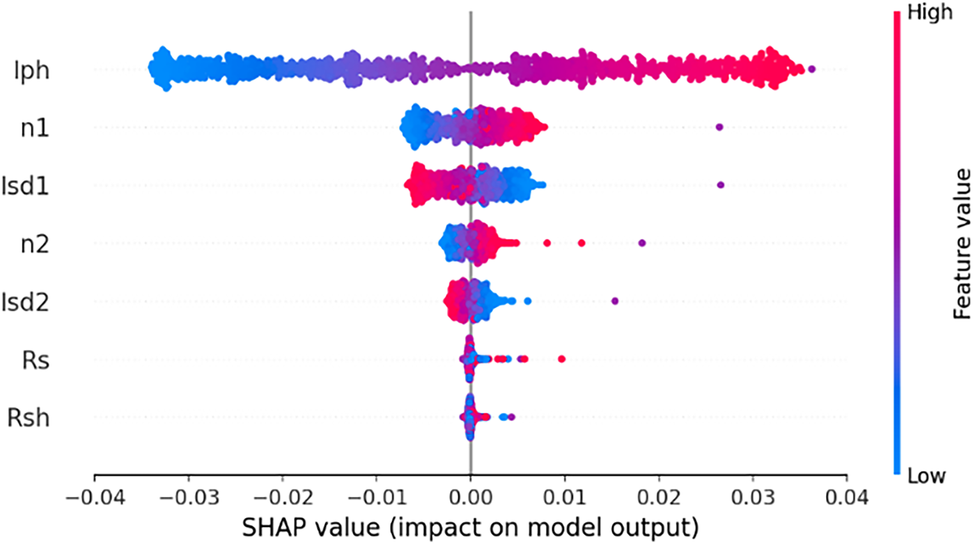
Figure 10: SHAP summary plot for the DDM.

In terms of effect direction, Iph exhibits a stable monotonic positive relationship. When Iph takes larger values, most samples fall in the positive SHAP region and increase the predicted output current. This observation is consistent with the SDM results. High-value samples of n1 and n2 more frequently appear on the positive side of the SHAP distribution, indicating that increasing the ideality factors generally leads to a slight increase in current, although their contributions are markedly smaller than that of Iph. In contrast, Isd1 and Isd2 show a “high-value, negative-contribution” tendency. Larger saturation currents are mostly associated with negative SHAP values and reduced output, whereas smaller values are more likely to yield positive contributions. Finally, Rs, and Rsh vary only slightly near zero, suggesting that they mainly play a fine-tuning role.

Overall, the SHAP summary plot for the DDM further corroborates the global sensitivity conclusions reported in the previous section. Iph remains the most critical dominant parameter, followed by the first-branch diode parameters n1 and Isd1. The added second-branch parameters n2 and Isd2 provide smaller yet physically meaningful corrections, whereas the resistive parameters Rs, and Rsh exhibit only very limited effects under specific operating conditions. These results indicate that, even when the model is extended from the single-diode to the double-diode form, the core sensitivity structure remains consistent, and SHAP offers a clearer and more interpretable picture of how each parameter contributes to the model output.

4  Conclusion

This study develops and validates a comprehensive framework that integrates parameter identification and global sensitivity analysis, improving both calibration accuracy and interpretability for equivalent-circuit photovoltaic models.

For parameter identification, SFOA is employed to calibrate the SDM and DDM. The regeneration mechanism enhances search flexibility, while the adaptive exploration regulation expands effective search coverage and mitigates premature convergence. The experimental results indicate that SFOA outperforms PSO, WOA, MGO, and JAYA in terms of RMSE, convergence stability, and computational efficiency. These findings demonstrate its strong capability in addressing highly nonlinear and coupled optimization problems in PV model calibration. Therefore, SFOA serves as a reliable foundational approach for parameter extraction prior to global sensitivity analysis. For sensitivity analysis, to alleviate the high computational burden of conventional approaches in high-dimensional parameter spaces, this study combines a RF surrogate with SHAP-based interpretability, enabling efficient sensitivity estimation within a physically plausible neighborhood. Therefore, the conclusions describe global sensitivities around the calibrated solution rather than universal global rankings across the full parameter domain. The global sensitivity results consistently indicate that the photocurrent Iph is the dominant parameter for both SDM and DDM, followed by the parameters of the first diode branch, while the resistive parameters exhibit limited influence within the ±5 percent neighborhood around the calibrated optimum considered in this work. Compared with MDI and OFAT, SHAP provides higher-resolution and more informative sensitivity interpretation in this study. MDI can offer a fast global ranking, but it may be affected by tree-splitting mechanisms and feature scale, and it does not directly convey effect direction. OFAT provides directional and marginal trends, yet it cannot capture parameter interactions or nonlinear condition-dependent effects due to the assumption that other parameters remain fixed. In contrast, SHAP delivers both near-optimum global importance ranking and sample-level additive attribution, revealing how effect direction and magnitude vary across operating points and highlighting conditional dependence. Its distribution-based visualizations further expose nonlinear patterns and interaction cues. Moreover, once the RF surrogate is trained, SHAP values can be computed efficiently by exploiting the tree structure, achieving strong interpretability without extensive repeated evaluations. The high predictive accuracy of the RF surrogate, as verified by RMSE and R2 on an independent test set, further supports the reliability of the sensitivity conclusions.

This study applies SHAP to the Random Forest surrogate, so the sensitivity conclusions depend on surrogate fidelity within the sampled neighborhood. Moreover, the analysis is confined to a ±5 percent region around the calibrated optimum to preserve physical plausibility, and the resulting rankings should not be directly extrapolated to wider parameter ranges or markedly different operating conditions. For more complex PV systems such as multi-module strings and arrays with mismatch or partial shading, the dimensionality of parameters and operating points can increase substantially, raising both the computational cost and the interpretive complexity of SHAP-based analysis. Future work will explore scalable extensions, including hierarchical or group-wise attributions, operating-region partitioning with piecewise surrogates, and feature grouping to maintain interpretability for multi-module settings.

Future work will extend to wider parameter domains and assess ranking stability beyond the near-optimum neighborhood. It should be noted that the present validation is conducted on a single R.T.C. France PV cell under standard test conditions (303.15 K and 1000 W/m2). Therefore, the calibration accuracy and sensitivity structures reported in this study are confined to this specific device and operating condition. While the proposed framework is methodologically general under the considered condition, its cross-condition and cross-device generalizability remains to be further verified. Overall, the proposed framework not only provides high-precision calibration for PV devices, but also offers data-driven and physically consistent sensitivity insights that support process optimization, fault diagnosis, and performance prediction with quantitative and engineering-relevant evidence.

Acknowledgement: The authors gratefully acknowledge the support and assistance provided by all individuals and institutions involved in this study.

Funding Statement: The authors received no specific funding for this study.

Author Contributions: Conceptualization, Yan-Hao Huang; methodology, Yan-Hao Huang; software and experiments, Yan-Hao Huang and Chung-Ming Kao; data analysis, Yan-Hao Huang; validation, Yan-Hao Huang; writing—original draft preparation, Yan-Hao Huang and Chung-Ming Kao; writing—review and editing, Yan-Hao Huang; supervision, Yan-Hao Huang. All authors reviewed and approved the final version of the manuscript.

Availability of Data and Materials: The data that support the findings of this study are available on request from the corresponding author.

Ethics Approval: Not applicable.

Conflicts of Interest: The authors declare no conflicts of interest.

References

1. Fahim SR, Hasanien HM, Turky RA, Abdel Aleem SHE, Ćalasan M. A comprehensive review of photovoltaic modules models and algorithms used in parameter extraction. Energies. 2022;15(23):8941. doi:10.3390/en15238941. [Google Scholar] [CrossRef]

2. Almalaq A, Harrison A, Alsaleh I, Alassaf A, Alangari M. Exact computer modeling of photovoltaic sources with lambert-W explicit solvers for real-time emulation and controller verification. Comput Model Eng Sci. 2026;146(1):1–10. doi:10.32604/cmes.2025.074815. [Google Scholar] [CrossRef]

3. Shaker LM, Al-Amiery AA, Hanoon MM, Al-Azzawi WK, Kadhum AAH. Examining the influence of thermal effects on solar cells: a comprehensive review. Sustain Energy Res. 2024;11(1):6. doi:10.1186/s40807-024-00100-8. [Google Scholar] [CrossRef]

4. Mlazi NJ, Mayengo M, Lyakurwa G, Kichonge B. Mathematical modeling and extraction of parameters of solar photovoltaic module based on modified Newton-Raphson method. Results Phys. 2024;57(3):107364. doi:10.1016/j.rinp.2024.107364. [Google Scholar] [CrossRef]

5. Et-torabi K, Nassar-eddine I, Obbadi A, Errami Y, Rmaily R, Sahnoun S, et al. Parameters estimation of the single and double diode photovoltaic models using a Gauss-Seidel algorithm and analytical method: a comparative study. Energy Convers Manag. 2017;148:1041–54. doi:10.1016/j.enconman.2017.06.064. [Google Scholar] [CrossRef]

6. Blaifi SA, Moulahoum S, Taghezouit B, Saim A. An enhanced dynamic modeling of PV module using Levenberg-Marquardt algorithm. Renew Energy. 2019;135(3):745–60. doi:10.1016/j.renene.2018.12.054. [Google Scholar] [CrossRef]

7. Saadaoui D, Elyaqouti M, Assalaou K, hmamou Ben D, Lidaighbi S. Parameters optimization of solar PV cell/module using genetic algorithm based on non-uniform mutation. Energy Convers Manag X. 2021;12(2):100129. doi:10.1016/j.ecmx.2021.100129. [Google Scholar] [CrossRef]

8. Lo WL, Chung HS, Hsung RT, Fu H, Shen TW. PV panel model parameter estimation by using particle swarm optimization and artificial neural network. Sensors. 2024;24(10):3006. doi:10.3390/s24103006. [Google Scholar] [PubMed] [CrossRef]

9. Ye X, Liu W, Li H, Wang M, Chi C, Liang G, et al. Modified whale optimization algorithm for solar cell and PV module parameter identification. Complexity. 2021;2021(1):8878686. doi:10.1155/2021/8878686. [Google Scholar] [CrossRef]

10. Tefek MF. Artificial bee colony algorithm based on a new local search approach for parameter estimation of photovoltaic systems. J Comput Electron. 2021;20(6):2530–62. doi:10.1007/s10825-021-01796-3. [Google Scholar] [CrossRef]

11. Yu WL, Wen CK, Liu EJ, Chang JY. Implementation of accurate parameter identification for proton exchange membrane fuel cells and photovoltaic cells based on improved honey badger algorithm. Micromachines. 2024;15(8):998. doi:10.3390/mi15080998. [Google Scholar] [PubMed] [CrossRef]

12. Liu EJ, Huang YH, Lin WL, Wen CK, Lin CI. Rapid, precise parameter optimization and performance prediction for multi-diode photovoltaic model using puma optimizer. Energies. 2025;18(11):2855. doi:10.3390/en18112855. [Google Scholar] [CrossRef]

13. Wu Z, Shen D. Parameter identification of photovoltaic cell model based on improved grasshopper optimization algorithm. Optik. 2021;247(1):167979. doi:10.1016/j.ijleo.2021.167979. [Google Scholar] [CrossRef]

14. Saltelli A. Sensitivity analysis: could better methods be used? J Geophys Res. 1999;104(D3):3789–93. doi:10.1029/1998jd100042. [Google Scholar] [CrossRef]

15. Morris MD. Factorial sampling plans for preliminary computational experiments. Technometrics. 1991;33(2):161–74. doi:10.1080/00401706.1991.10484804. [Google Scholar] [CrossRef]

16. Saltelli A, Annoni P, Azzini I, Campolongo F, Ratto M, Tarantola S. Variance based sensitivity analysis of model output. Design and estimator for the total sensitivity index. Comput Phys Commun. 2010;181(2):259–70. doi:10.1016/j.cpc.2009.09.018. [Google Scholar] [CrossRef]

17. Ibrahim IA, Hossain MJ, Duck BC. An optimized offline random forests-based model for ultra-short-term prediction of PV characteristics. IEEE Trans Ind Inf. 2020;16(1):202–14. doi:10.1109/tii.2019.2916566. [Google Scholar] [CrossRef]

18. Wang H, Liang Q, Hancock JT, Khoshgoftaar TM. Feature selection strategies: a comparative analysis of SHAP-value and importance-based methods. J Big Data. 2024;11(1):44. doi:10.1186/s40537-024-00905-w. [Google Scholar] [CrossRef]

19. Harrison A. PILoN: physics-informed logistic nonlinear model for photovoltaic performance modelling. Energy Rep. 2026;15:109026. doi:10.1016/j.egyr.2025.109026. [Google Scholar] [CrossRef]

20. Xu J, Zhou C, Li W. Photovoltaic single diode model parameter extraction by dI/dV-assisted deterministic method. Sol Energy. 2023;251:30–8. doi:10.1016/j.solener.2023.01.009. [Google Scholar] [CrossRef]

21. Saltelli A, Aleksankina K, Becker W, Fennell P, Ferretti F, Holst N, et al. Why so many published sensitivity analyses are false: a systematic review of sensitivity analysis practices. Environ Model Softw. 2019;114(1):29–39. doi:10.1016/j.envsoft.2019.01.012. [Google Scholar] [CrossRef]

22. Liu X, Yang H, Shen C, Lu L, Wang J. Quantifying the parameter interaction of photovoltaic double skin façade: a sensitivity analysis based on second-order Morris method. Appl Energy. 2025;386:125579. doi:10.1016/j.apenergy.2025.125579. [Google Scholar] [CrossRef]

23. Zhong C, Li G, Meng Z, Li H, Yildiz AR, Mirjalili S. Starfish optimization algorithm (SFOAa bio-inspired metaheuristic algorithm for global optimization compared with 100 optimizers. Neural Comput Appl. 2025;37(5):3641–83. doi:10.1007/s00521-024-10694-1. [Google Scholar] [CrossRef]

24. Liu EJ, Chen RW, Wang QA, Lu WL. Shuffled puma optimizer for parameter extraction and sensitivity analysis in photovoltaic models. Energies. 2025;18(15):4008. doi:10.3390/en18154008. [Google Scholar] [CrossRef]

25. Ourbih-Tari M, Guebli S. A comparison of methods for selecting values of simulation input variables. ESAIM Probab Stat. 2015;19:135–47. doi:10.1051/ps/2014020. [Google Scholar] [CrossRef]

26. Schuck de Oliveira F, Perin Gasparin F, Detzel Kipper F, Krenzinger A. An alternative method to IEC 60891 standard for I−V curve correction based on a single measurement. Sol Energy. 2024;284:113067. doi:10.1016/j.solener.2024.113067. [Google Scholar] [CrossRef]

27. Dirnberger D, Kräling U. Uncertainty in PV module measurement: part I: calibration of crystalline and thin-film modules. IEEE J Photovolt. 2013;3(3):1016–26. doi:10.1109/JPHOTOV.2013.2260595. [Google Scholar] [CrossRef]

28. Gulkowski S, Krawczak E. Thin-film photovoltaic modules characterisation based on I-V measurements under outdoor conditions. Energies. 2024;17(23):5853. doi:10.3390/en17235853. [Google Scholar] [CrossRef]