
 Login
Login Register
 Submit a Paper
 Propose a Special lssue
 Open Access
ARTICLE
A Lightweight Dual-Branch CNN with Frequency Domain Perception Loss for Image Denoising
SWJTU-Leeds Joint School, Southwest Jiaotong University, Chengdu, China
* Corresponding Author: Yufeng Qin. Email:
(This article belongs to the Special Issue: Super-Resolution for Remote Sensing, Medicine and Intelligent Vision Systems)
Computers, Materials & Continua 2026, 89(2), 67 https://doi.org/10.32604/cmc.2026.084385
Received 21 April 2026; Accepted 11 August 2026; Issue published 15 September 2026
 View Full Text
 Download PDF
Abstract
Lightweight real-time image denoising is crucial for resource-constrained edge devices, yet existing compact convolutional neural networks (CNNs) often lose high-frequency details due to limited capacity and the absence of explicit frequency-domain supervision. This paper proposes a 0.18M-parameter dual-branch denoising network driven by a novel Frequency Domain Perception Loss (FDPL). The architecture decouples noise removal and detail recovery via a low-frequency branch composed of four Residual-in-Residual Dense Blocks (RRDB) and a high-frequency branch with two Residual Channel Attention Blocks (RCAB). The composite loss combines brightness-aware Mean Square Error (MSE), Visual Geometry Group 19-layer (VGG19) perceptual loss, and the FDPL, which applies a circular mask in the frequency domain (high/low weights of 0.8/0.2) with linear warm-up. Extensive experiments on Berkeley Segmentation Dataset with 68 images (BSD68), its color counterpart (CBSD68), and Urban100 (100 high-resolution urban scene images) demonstrate the model’s effectiveness: the FDPL consistently improves Peak Signal-to-Noise Ratio (PSNR) by 0.37–0.69 dB across all datasets, pushing the peak performance to 31.37 dB on BSD68, which surpasses classic Denoising Convolutional Neural Network (DnCNN) by 5.28 dB. When further evaluated against recent state-of-the-art lightweight models on the Berkeley Segmentation Dataset (500 images) (BSD500) benchmark under both low and moderate noise levels, our method achieves highly competitive results–31.15 dB PSNR at σ = 12.75, approaching the much larger Real Image Denoising Network (RIDNet) (32.34 dB) while being over five times smaller and exhibiting 7.4× faster inference. It surpasses SwinIR-light by 0.28 dB with 33× lower latency at σ = 12.75 and maintains comparable accuracy with over 30× speedup at σ = 25. With only 0.18M parameters and 3.29 ms Central Processing Unit (CPU) inference per 64 × 64 patch, the model is readily deployable on edge devices. Ablation studies confirm the importance of both the dual-branch design and the FDPL. These results highlight that the proposed architecture and loss function enable an ultra-lightweight CNN to rival significantly heavier models, making it particularly suitable for real-time denoising in resource-limited applications such as mobile imaging, surveillance, and on-device preprocessing.Keywords
Image denoising is a fundamental low-level vision task that aims to recover a high-fidelity clean image from noisy observations. Its restoration quality strongly influences the accuracy of subsequent high-level tasks such as object detection, semantic segmentation, and image classification, and it serves as a critical preprocessing step for industrial applications including surveillance imaging, medical image analysis, and visual perception on edge devices. In resource-constrained edge computing environments, the ability to perform real-time denoising with minimal computational overhead is particularly crucial, as it directly affects the responsiveness and reliability of the entire vision pipeline.
Early image denoising methods were dominated by model-driven algorithms such as interpolation filtering, total variation minimization, non-local means [1], and the classic Block-Matching and 3D filtering (BM3D) algorithm [2]. These methods are valued for their low computational cost and mathematical tractability, making them suitable for resource-limited scenarios. However, their performance relies heavily on hand-crafted priors, which often fail to capture the complexity of real-world noise. More importantly, these schemes operate primarily in the spatial domain and cannot effectively separate high-frequency details (edges, textures, fine contours) from random noise. Consequently, they either leave noise unresolved or, in trying to suppress it, cause severe texture erosion and over-smoothing, limiting their adequacy for high-fidelity reconstruction.
With the progress of deep learning [3], convolutional neural networks (CNNs) have become the dominant paradigm for image denoising, achieving substantial gains over traditional algorithms. Denoising Convolutional Neural Network (DnCNN) [4] introduced residual learning and batch normalization (BN), enabling efficient end-to-end Gaussian denoising. Image Restoration Convolutional Neural Network (IRCNN) [5] further incorporated dilated convolutions to enlarge the receptive field without extra computational cost and integrated explicit image priors for better adaptability to varying noise levels. These models set new benchmarks and demonstrated the potential of deep CNNs for low-level vision tasks—a success originally shown by large-scale image classification [6]. More recently, lightweight CNN and transformer-based models have been developed for efficient image restoration on resource-constrained platforms [7,8]. However, these designs primarily target architectural compactness, and multi-frequency features are still processed through shared pathways without explicit frequency-wise decoupling, leaving fine-grained texture recovery largely unoptimized under tight parameter constraints.
For both classic deep denoisers and latest lightweight models, the root cause of this texture loss lies in their unified single-branch design, which processes low-frequency and high-frequency information through shared convolutional layers. This design tends to couple noise suppression with detail preservation, making it difficult to remove noise without simultaneously smoothing out fine textures and sharp edges. As a result, these models frequently produce over-smoothed outputs where important high-frequency details are lost—a weakness especially harmful for high-fidelity downstream tasks.
To address this limitation, recent work has explored multi-branch architectures that separate feature extraction into distinct pathways. For example, Dual-branch UNet with Information Exchange (DuINet) introduces a dual-branch structure with information exchange to balance noise removal and detail retention, while Dual-Branch Feature Extraction Network (DBFE-Net) targets Gaussian blind denoising with a dedicated dual-branch design [9,10]. The broader principle that enhanced feature representations benefit image restoration has also been extensively validated in super-resolution research [11]. These efforts demonstrate that architectural innovations—particularly explicit feature decoupling—help mitigate the trade-off between denoising and detail preservation. Building on this insight, we construct a dual-branch network that directs low-frequency components to Residual-in-Residual Dense Blocks (RRDB), a design first introduced in Enhanced Super-Resolution Generative Adversarial Network (ESRGAN) and subsequently widely adopted in image restoration [12], and high-frequency details to Residual Channel Attention Blocks (RCAB) that exploit channel attention mechanisms prevalent in modern super-resolution and restoration architectures [13].
In terms of loss function design, the Mean Squared Error (MSE) loss has long been the de facto choice for denoising models, thanks to its stability and simplicity. However, MSE operates purely in the spatial domain, focusing on global error minimization and providing insufficient constraints on high-frequency components, which often leads to over-smoothed outputs with lost textures and edges. To address this, perceptual loss was introduced to low-level vision tasks, leveraging pre-trained Visual Geometry Group (VGG) networks as widely adopted in deep learning literature [14]; it computes distance in their feature space, yielding visually more natural results. Nevertheless, both MSE and perceptual loss remain fundamentally spatial or semantic, lacking explicit frequency-domain constraints to penalize high-frequency detail attenuation.
Loss functions beyond conventional MSE have been widely explored in image restoration [15]. Frequency-domain losses have recently been proposed to reweight different spectral components for detail retention [16]. However, most existing methods use rectangular masks that may cause spectral leakage. To address this, we propose a circular-mask Frequency Domain Perception Loss (FDPL), which more accurately separates frequency bands and is combined with a brightness-aware reweighting, explicitly penalizes high-frequency attenuation without sacrificing structural fidelity. Recent lightweight restoration studies [17,18] have also validated the value of frequency-aware learning for detail retention, yet most only embed frequency priors implicitly in feature extraction, without explicit weighted spectral constraints in the loss optimization stage.
A large body of lightweight denoising architectures prioritize reducing parameter counts at the cost of sacrificing texture restoration capability, while frequency-aware restoration methods usually adopt heavy computational pipelines that cannot be deployed on low-power embedded hardware simultaneously. Despite continuous progress in both architectural design and loss function optimization, most existing methods still struggle to jointly address three key requirements: explicit frequency-domain supervision, robust detail recovery under challenging lighting, and compactness for edge deployment. Moreover, many high-performing models contain millions of parameters, rendering them impractical for resource-constrained devices such as surveillance cameras or mobile phones. This growing demand for real-time, lightweight denoising in applications like autonomous driving and medical imaging calls for a more integrated solution.
To bridge these gaps, we introduce a dual-branch convolutional network that keeps noise suppression and detail recovery in separate processing paths. One branch, built with four Residual-in-Residual Dense Blocks, reconstructs a clean low-frequency base; the other, composed of two lightweight Residual Channel Attention Blocks, selectively reinforces high-frequency structures such as edges and textures. The model is trained with a composite loss that combines a brightness-aware pixelwise term, a VGG-based perceptual term, and our proposed Frequency Domain Perception Loss. FDPL transforms images into the frequency domain and applies a circular mask—rather than a rectangular one—to weight different spectral components, thereby directly penalizing high-frequency attenuation and preserving fine textures that conventional losses tend to smooth away. The entire network contains only 0.18M parameters and processes a 64 × 64 patch in 3.29 ms on a consumer Central Processing Unit (CPU), making it practical for resource-limited edge devices. In experiments across multiple benchmarks, this lightweight design consistently approaches or exceeds the accuracy of much larger denoisers while keeping real-time throughput. Ablation studies further confirm that both the dual-branch architecture and the FDPL are essential for the observed gains, demonstrating that careful architectural choices combined with frequency-aware supervision can effectively balance denoising quality and computational efficiency.
The remainder of this paper is organized as follows. Section 2 details the proposed dual-branch network architecture and the composite FDPL loss. Section 3 describes the experimental setup, benchmark datasets, and both quantitative and qualitative results. Section 4 discusses the principal findings, ablation analyses, and current limitations. Section 5 concludes the paper and outlines future research directions.
The proposed model is implemented based on PyTorch, and its overall workflow is illustrated in Fig. 1. Specifically, Fig. 1a depicts the training process, where the model learns to map noisy input images to clean outputs by minimizing a multi-loss objective. Fig. 1b shows the inference pipeline for a single image, which follows a sliding-window strategy to handle arbitrary-sized inputs efficiently. As shown in Fig. 1a, the noisy input is first normalized to [−1, 1] (mean = 0.5, std = 0.5) to align with the network’s activation functions. It then enters a shared 3 × 3 convolution (stride 1, padding 1) that maps the red, green and blue (RGB) input to a 32-dimensional feature space, providing a compact yet expressive representation.
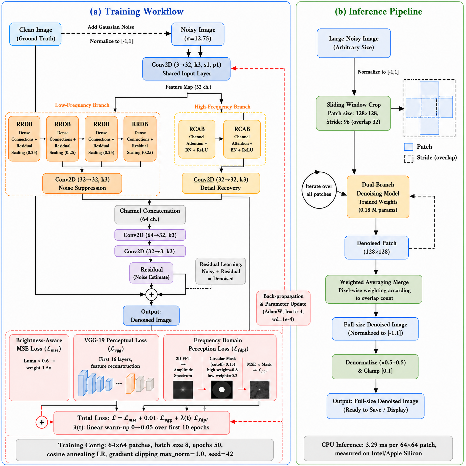
Figure 1: Overall workflow of the proposed dual-branch FDPL image denoising model. (a) Training workflow; (b) Inference pipeline.
The features are then fed into two specialized branches. The low-frequency branch is composed of four stacked RRDBs, each employing dense connections and a residual scaling factor of 0.25. The high-frequency branch consists of two lightweight RCABs, each comprising two convolutional layers with batch normalization and a channel attention mechanism. After the dual-branch processing, the output features from both branches are concatenated along the channel dimension, resulting in a 64-dimensional feature map. A 3 × 3 convolution fuses these features and restores the channel count to 32. A second 3 × 3 convolution then maps the result to RGB space, producing a residual image. As common in image denoising, the network predicts the noise residual rather than the clean image directly. The final denoised output is obtained by adding this residual to the original input noisy image. This simplifies the learning objective and improves training stability, especially for deep networks.
For inference on images larger than the training patch size (64 × 64), we adopt a sliding-window approach as shown in Fig. 1b. The input image is divided into overlapping patches of size 128 × 128 with a stride of 96 (i.e., an overlap of 32 pixels) to avoid boundary artifacts. Each patch is normalized and passed through the model independently. The denoised patches are then aggregated by weighted averaging according to the number of overlapping contributions at each pixel position, yielding a seamless full-size output. This enables efficient high-resolution processing while maintaining consistent denoising quality.
2.2 Specialized Dual-Branch Architecture
The overall architecture and the internal structures of the RRDB and RCAB modules are illustrated in Fig. 1. As shown in Fig. 1, the RRDB module was originally introduced in ESRGAN [12], and it has been widely adopted in subsequent restoration work; the RCAB design leverages channel-wise attention strategies like those explored in recent feature modulation networks. The core of the model lies in its dual-branch design, which explicitly separates the processing of low-frequency structural information and high-frequency detail information. This separation is achieved through two specialized modules: the RRDB for the low-frequency branch and the RCAB for the high-frequency branch.
The low-frequency branch consists of four stacked RRDB modules, and each RRDB module is composed of three convolutional layers. The first convolutional layer applies a 3 × 3 kernel (padding 1) to the input feature map (32 channels) and expands it to 16 channels, followed by a Leaky Rectified Linear Unit (LeakyReLU) activation (negative slope = 0.2). The second convolution concatenates the original input with the output of the first layer (now 48 channels) and again produces 16 channels, also followed by LeakyReLU. The third convolution takes the concatenation of the original input and the outputs of both previous layers (64 channels) and reduces it back to 32 channels, generating a residual feature map. This residual is scaled by a factor of 0.25 before being added to the input, forming a residual connection. The dense connectivity pattern and residual scaling together enhance feature expression, facilitate gradient flow, and enable the branch to effectively remove low-frequency Gaussian noise while reconstructing the clean image base.
The high-frequency branch comprises two lightweight RCAB modules. Each RCAB module contains a feature extraction path composed of two 3 × 3 convolutional layers, each followed by batch normalization and a Rectified Linear Unit (ReLU) activation. This path extracts local features that are critical for edge and texture recovery. Parallel to this, a channel attention path computes channel-wise importance weights: global average pooling compresses spatial information to 1 × 1, followed by two 1 × 1 convolutions that first reduce the channel dimension from 32 to 8 and then restore it to 32. A Sigmoid activation produces a weight vector that is multiplied elementwise with the feature map from the feature extraction path. The resulting weighted feature map is added back to the input of the module, forming a residual connection. This attention mechanism adaptively emphasizes high-frequency details (e.g., edges, textures) while suppressing redundant information, enabling precise detail restoration.
This specialized division of labor between the two branches addresses the core limitation of conventional single-branch architectures. Unlike unified networks that force the same convolutional kernels to learn both noise suppression and detail recovery, our design allows each branch to optimize for a single, well-defined objective. The low-frequency branch can prioritize smooth, stable feature learning for noise removal without being constrained by the need to preserve sharp details, while the high-frequency branch focuses exclusively on enhancing sparse, fine-grained features without being affected by global noise distribution. This decoupling mitigates the inherent trade-off between denoising and detail preservation in traditional designs.
2.3 Weighted Fusion Strategy for Multiple Losses
To guide the model toward high-quality denoising while preserving fine details and perceptual naturalness, we employ a multi-loss weighted fusion strategy. The total loss function is defined as a linear combination of three complementary terms:
where λ(t) is a dynamic weight that follows a linear warm-up schedule during the first 10 training epochs, increasing from 0 to 0.05 and then remaining constant. This schedule ensures that the FDPL loss does not dominate the early training phase, allowing the model to first learn stable noise suppression before being heavily guided by high-frequency constraints.
2.3.1 Luminance-Aware MSE Loss
Conventional MSE loss treats all pixels uniformly, which often leads to suboptimal performance in high-brightness regions where noise is more perceptible. To address this, we design a luminance-aware MSE loss. The pixel luminance is calculated using the International Telecommunication Union Radiocommunication Sector (ITU-R) Recommendation BT.601 grayscale conversion formula Y = 0.299R + 0.587G + 0.114B. A weight of 1.5× is applied to loss terms corresponding to pixels with luminance values greater than 0.6, thereby strengthening the model’s denoising optimization for high-brightness regions and avoiding distortion in these areas. The loss function is formulated as:
In Eq. (2),
To enhance the visual naturalness of the output images, we adopt the Visual Geometry Group 19-layer (VGG19) network pre-trained on the ImageNet (1000-class) classification dataset (ImageNet1K). The first 16 layers of its feature extraction module are selected to construct the perceptual loss; all weights of this part are frozen during training, and the module is only used for extracting high-level semantic features. By minimizing the feature-space difference between the predicted and ground-truth images, the model is guided to restore image content consistent with human visual perception. Since the pre-trained VGG19 weights are optimized for RGB images in the range [0, 1], the model outputs (normalized to [−1, 1]) are renormalized to [0, 1] (
where
2.3.3 Frequency Domain Perception Loss
To strengthen the model’s constraint on high-frequency details, we design the Frequency Domain Perception Loss (FDPL). The image is transformed to the frequency domain via 2D Fast Fourier Transform (FFT), and the amplitude spectrum is calculated. A circular mask is used to separate the low-frequency region (central circular area) and high-frequency region (peripheral area), with weights of 0.2 and 0.8 assigned to low-frequency and high-frequency loss terms, respectively. This design imposes differential constraints on low and high-frequency components, forcing the model to accurately restore high-frequency details while suppressing noise. The loss function is formulated as:
where
In our implementation, the cutoff ratio for the circular mask is set to 0.15 (i.e., the radius of the low-frequency circle is 15% of the maximum spectral distance). This ratio is chosen empirically to balance structural integrity and detail preservation.
Together, the three loss terms form a multi-scale constraint system spanning the pixel, semantic, and frequency domains. The brightness-aware MSE ensures luminance fidelity and specifically improves restoration in high-brightness areas; the VGG19 perceptual loss provides semantic supervision that aligns outputs with human visual perception; and the FDPL imposes explicit frequency-domain constraints that directly penalize high-frequency attenuation. This joint optimization enables the model to simultaneously balance global structural accuracy, visual naturalness, and fine-grained detail preservation, avoiding the over-smoothing tendency of MSE-only training.
3.1.1 Dataset and Data Preprocessing
Datasets. Four widely used public benchmarks are employed in this study. The Berkeley Segmentation Dataset with 68 images (BSD68) contains 68 grayscale natural images covering diverse scenes; the Color Berkeley Segmentation Dataset with 68 images (CBSD68) is its color counterpart with 68 color images; the Urban100 dataset consists of 100 high-resolution urban scenes rich in edges and fine textures. These three datasets are used for ablation experiments and comparisons with classic baselines. All three datasets are randomly split into training and validation sets with an 8:2 ratio. No separate test set is used, and all quantitative evaluations are performed on the validation split. For fair comparison with recent lightweight state-of-the-art models, we additionally employ the Berkeley Segmentation Dataset with 500 images (BSD500), which contains 200 training and 100 validation natural scene images. In the state-of-the-art experiments, we strictly follow the official training/validation split. Table 1 summarizes the key characteristics of each dataset, and Fig. 2 (representative samples) provides a visual overview of the image content from each dataset.
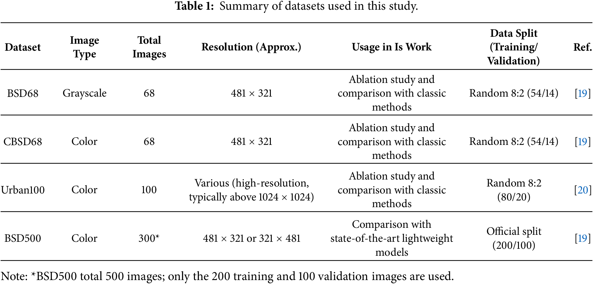

Figure 2: Representative image samples from the four datasets used in this study. (a) BSD68, a grayscale natural image; (b) CBSD68, a color image from the same scene family; (c) Urban100, a high-resolution urban scene with abundant edges and textures; (d) BSD500, a typical color natural image from the official training/validation split.
Data Preprocessing and Training Configuration. The complete pipeline from raw images to training samples is illustrated in Fig. 3. Each clean image is first corrupted by additive white Gaussian noise (AWGN) at σ = 12.75; for the BSD500 benchmark, we also evaluate at σ = 25. The noisy images are then randomly cropped into 64 × 64 patches and normalized to the range [−1, 1] using mean [0.5, 0.5, 0.5] and standard deviation [0.5, 0.5, 0.5]. For BSD68, CBSD68, and Urban100, the dataset is randomly partitioned into training (80%) and validation (20%) sets; for BSD500, the official split (200 training/100 validation) is adopted. Finally, the patches are organized into mini-batches of size 8 with shuffling enabled for training and disabled for validation.
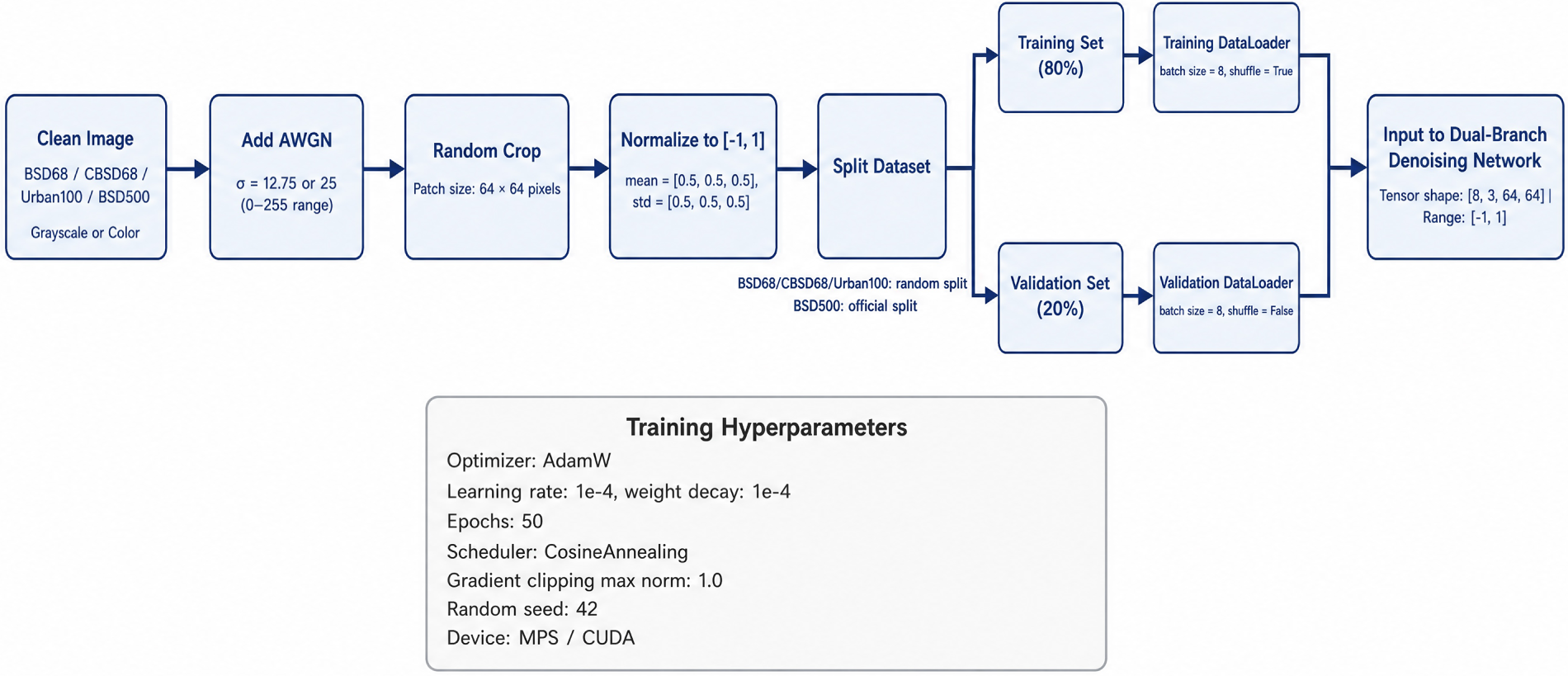
Figure 3: Data preprocessing pipeline from raw images to training samples. Key parameters are annotated in each step.
The model is optimized with Adaptive Moment Estimation with Decoupled Weight Decay (AdamW) using an initial learning rate of 1 × 10⁻⁴ and weight decay of 1 × 10⁻⁴. Training lasts 50 epochs with a cosine annealing learning rate scheduler and gradient clipping at max norm 1.0 to stabilize training. The random seed is fixed at 42 to guarantee complete reproducibility. All training hyperparameters are also summarized in the supplementary block of Fig. 3.
We quantitatively evaluate denoising performance using peak signal-to-noise ratio (PSNR) and structural similarity index measure (SSIM) [21]. SSIM is computed with the standard sliding-window method (Gaussian kernel, window size = 11, σ = 1.5) as defined in [21], guaranteeing a rigorous perceptual assessment; future work may also incorporate no-reference quality indicators [22]. All reported SSIM values have been recalculated with this standard implementation to ensure consistency across experiments.
For the ablation study, we compare against two classic CNN denoisers, DnCNN and IRCNN, as well as our own variants (Plain Convolution (PlainConv), swapped branches, and Ours without FDPL). For the state-of-the-art comparison on BSD500, we re-train three recent lightweight models—Fast and Flexible Denoising Network (FFDNet) [23], Real Image Denoising Network (RIDNet) [24], and a lightweight Swin Transformer for Image Restoration (SwinIR) variant [25]—using the same training configuration described above. All three models were retrained using the same composite loss as Ours w/o FDPL, i.e., brightness-aware MSE + VGG perceptual loss without the FDPL term, to isolate the architectural contribution. These models were chosen because they represent the most competitive lightweight architectures in the literature.
3.2 Experiment Results and Analysis
3.2.1 Ablation Study and Comparison with Classic Baselines
Table 2 reports the quantitative results on BSD68, CBSD68, and Urban100. The full model (Ours w/FDPL) achieves the best performance across all three datasets, surpassing DnCNN and IRCNN by over 5 dB on BSD68. The FDPL loss consistently improves PSNR by 0.37–0.69 dB, with the most pronounced gain on BSD68, where the balanced mixture of low-frequency and high-frequency content benefits most from explicit frequency-domain supervision. On Urban100, already dominated by fine textures, the contribution is smaller but still positive.
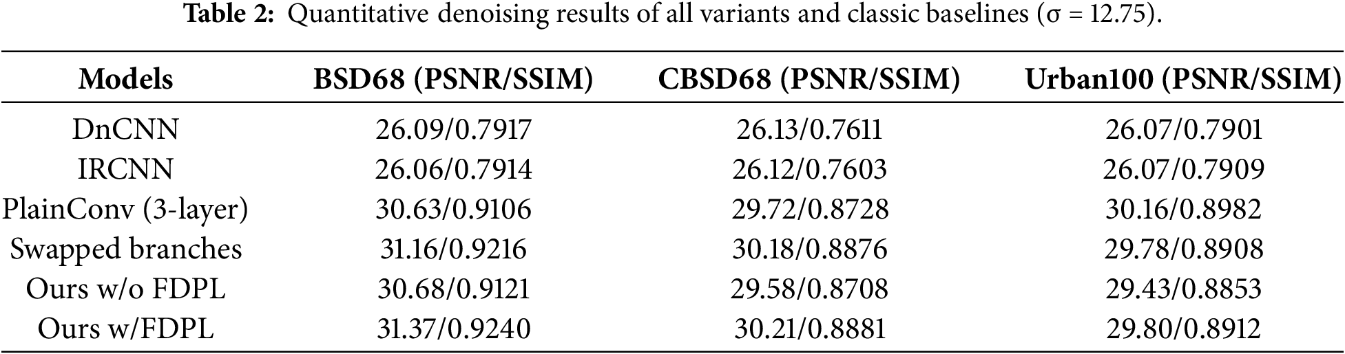
The swapped-branch variant slightly underperforms the original architecture on all datasets (e.g., 31.16 vs. 31.37 dB on BSD68), confirming that the default pairing (RRDB for low-frequency, RCAB for high-frequency) is optimal. The plain convolution variant suffers a clear performance drop on BSD68 (30.63 dB) and CBSD68 (29.72 dB) yet attains a deceptively high PSNR on Urban100 (30.16 dB). As will be discussed in Section 3.3.2, this anomaly arises from overfitting to repetitive urban textures, not from genuine denoising capability.
3.2.2 Comparison with State-of-the-Art Lightweight Models on BSD500
To assess the competitiveness of our method against recent lightweight architectures, we trained and evaluated FFDNet, RIDNet, and SwinIR-light on the BSD500 dataset under the same protocol. Table 3 summarizes the results, together with parameter counts and CPU inference times (measured on a single 64 × 64 patch). At σ = 12.75, our model achieves 31.15 dB, which is only 1.19 dB below the much larger RIDNet (32.34 dB) while having 5× fewer parameters and 7.4× faster inference. Against the ultra-lightweight SwinIR-light, our model delivers 0.28 dB higher PSNR and runs 33× faster (3.29 vs. 109.03 ms). At σ = 25, the PSNR of our model (27.57 dB) is very close to that of SwinIR-light (27.61 dB) and still largely outperforms FFDNet (24.30 dB). These numbers confirm that the proposed dual-branch CNN with FDPL offers an excellent balance between denoising accuracy and real-time efficiency, making it particularly suitable for resource-constrained edge devices.
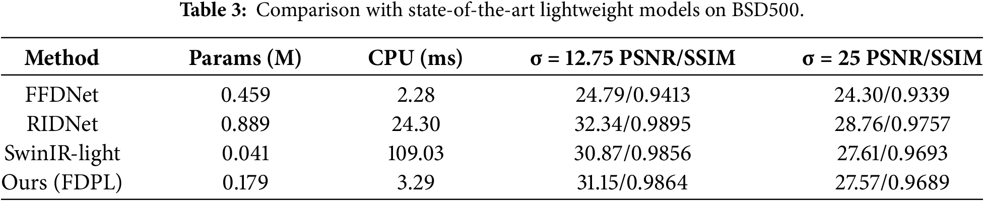
CPU time is measured on a 64 × 64 patch on a single core of an Apple M5 Pro System on Chip (SoC) (CPU only, PyTorch, no Metal Performance Shaders (MPS)/Graphics Processing Unit (GPU) acceleration). The exact parameter count of our model is 0.179M; 0.18M is used in the text for readability. A detailed qualitative comparison with example images is provided in Section 3.4.
3.3 Ablation Study on Architecture and Module Design
To further validate the design choices, we conduct two strictly controlled ablation experiments. All variants share the same training configuration, with only the architectural component under test modified. For a fair ablation, all variants share the identical backbone architecture except where explicitly stated. The key differences in training configuration are summarized below.
Ours w/FDPL (full model): Trained with the composite,
3.3.1 Module-Branch Pairing Optimality
We swap the module assignments: the low-frequency branch is replaced by 2 RCAB modules, and the high-frequency branch by 4 RRDB modules. As shown in Table 2, the swapped model obtains 31.16 dB on BSD68, 30.18 dB on CBSD68, and 29.78 dB on Urban100, consistently equal to or slightly worse than the original design (−0.21, −0.03, and −0.02 dB, respectively). This confirms that the original pairing is the most effective among the configurations tested, as RRDB’s dense connections are better suited for global noise suppression, while RCAB’s channel attention selectively enhances sparse high-frequency details.
3.3.2 Necessity of Specialized Modules and Overfitting Analysis
When both branches are replaced with plain 3-layer convolutions (no residual connections, dense connections, or attention), the PSNR drops to 30.63 dB on BSD68 (−0.74 dB) and 29.72 dB on CBSD68 (−0.49 dB). On Urban100, however, this plain variant reaches 30.16 dB, slightly higher than Ours w/FDPL (29.80 dB). This apparent anomaly is the result of dataset-specific overfitting: the repetitive brick and window textures in Urban100 can be superficially memorized by the plain convolution block, but the gain disappears entirely on datasets with more diverse content. The training curves further confirm this behavior: the plain model’s validation PSNR plateaus at epoch 29 and never improves, whereas our model continues to learn stably throughout the full 50 epochs. These observations demonstrate that the specialized RRDB and RCAB modules not only boost performance but also provide a strong regularization effect that prevents overfitting and ensures generalizable denoising capability.
The plain convolution variant’s anomalous gain on a single dataset should not be misinterpreted as a sign of superiority. Instead, it emphasizes the critical importance of evaluating denoising methods on diverse, general-purpose benchmarks. Our model is designed to serve as a reliable lightweight denoising engine for edge-deployment scenarios, where robustness and generalization are paramount. It maintains state-of-the-art results on BSD68 and CBSD68 while running in real time on a CPU, making it considerably more practical than a model that performs well only on a narrow class of textures. This design philosophy aligns with the demanding requirements of applications such as mobile imaging, surveillance, and on-device preprocessing.
3.4 Qualitative Visual Analysis
To complement the quantitative metrics, we provide a comprehensive visual assessment covering detail preservation, robustness under challenging lighting, efficiency trade-offs, and current limitations.
3.4.1 Detail Preservation and FDPL Effectiveness
Fig. 4 presents the full-image denoising results on a representative brick wall scene from Urban100 (σ = 12.75). The noisy input (Fig. 4a) is severely corrupted; the model without FDPL (Fig. 4b) removes most of the noise but introduces noticeable blur along brick edges and essentially erases the fine granular texture of the brick surface. In contrast, the full model with FDPL (Fig. 4c) preserves sharp edges and the natural roughness of the material, yielding a visual result far closer to the noise-free ground truth.
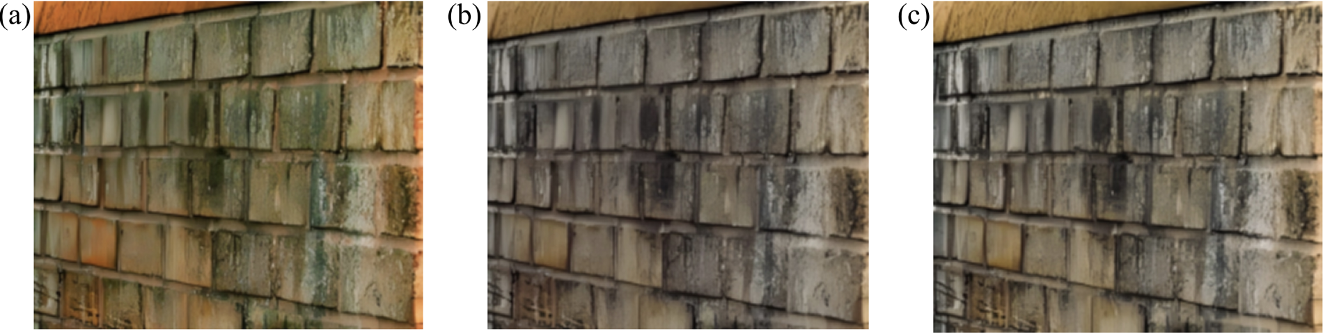
Figure 4: Comparison of denoising effects for brick wall scenes in Urban100 dataset. (a) Noisy input image; (b) Dual-branch model without FDPL; (c) Dual-branch model with FDPL in this paper.
A more detailed inspection is provided in Fig. 5. Fig. 5a displays zoomed-in image patches of the same brick wall scene alongside their corresponding pixel-wise error heatmaps, all rendered under a unified color scale where darker tones represent lower mean absolute error (MAE). The w/o FDPL patch appears smeared and pastel-like, and its error map is dominated by bright, high-intensity pixels, indicating persistently high reconstruction error across the textured region. In stark contrast, the w/FDPL patch retains the crisp, irregular grain of the brick, and its error map is visibly darker, reflecting a substantially lower MAE. The improvement is most pronounced along brick edges and within the granular surface—precisely where the model without FDPL fails.
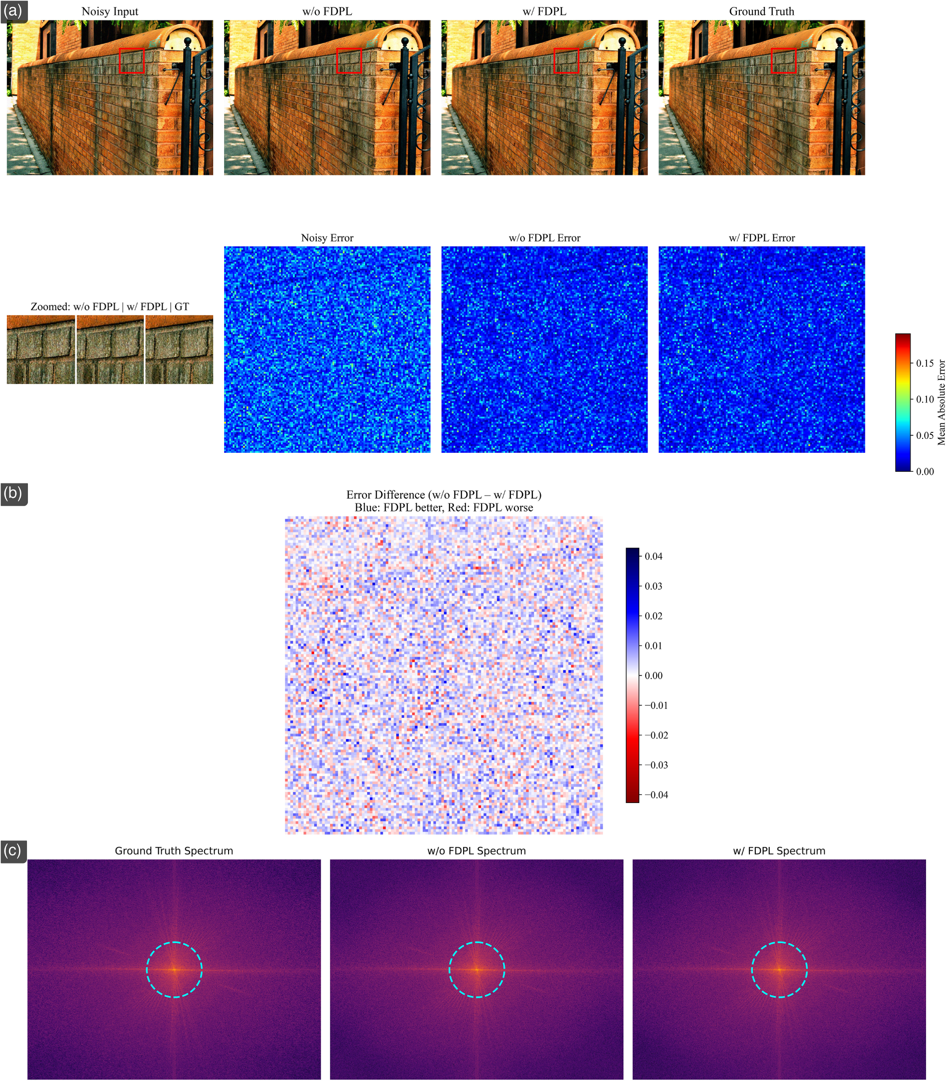
Figure 5: Detailed error analysis on the brick wall scene (Urban100, σ = 12.75). (a) From left to right: zoomed-in patches of w/o FDPL, w/FDPL, and ground truth, with corresponding error maps under a unified color scale; (b) Error difference map (w/o FDPL − w/FDPL); blue indicates lower error; (c) Log-scale amplitude spectra; the dashed circle marks the low-frequency region (cutoff = 0.15).
Fig. 5b further reinforces this observation by showing the pixel-wise error difference map (w/o FDPL − w/FDPL). In this representation, blue pixels correspond to locations where FDPL reduces the reconstruction error (i.e., performs better), while red pixels indicate the opposite. The difference map is overwhelmingly dominated by blue, demonstrating that FDPL brings a widespread and consistent improvement in fidelity. The sparse red regions are confined to flat, homogeneous areas where both models already achieve negligible error. This visual evidence directly corroborates the quantitative PSNR gains reported in Table 2 and provides an intuitive explanation for how the frequency-domain loss counteracts the over-smoothing tendency inherent in MSE-driven training.
A complementary spectral perspective is given in Fig. 5c, which compares the 2D amplitude spectra of the denoised outputs. The model with FDPL retains noticeably more energy in the high-frequency region, closely matching the ground truth spectrum, whereas the model without FDPL shows a clear attenuation of high-frequency components. This spectral behavior provides a mechanistic explanation for the over-smoothed appearance observed in the spatial domain: without the FDPL constraint, the network’s optimization naturally suppresses frequencies that carry fine textural information. Our proposed FDPL loss addresses this issue by assigning higher penalties to high-frequency components, explicitly guiding the network to preserve fine textures. Together, the spatial and spectral evidence in Fig. 5 confirms that FDPL effectively compels the network to preserve perceptually critical high-frequency structures.
3.4.2 Robustness under Challenging Lighting
Fig. 6 shows a low-illumination high-noise urban scene captured at night (Apple iPhone 15 Pro Max, International Organization for Standardization (ISO) 12500, 1/15 s exposure, f/1.78), which poses a severe challenge for both denoising and detail preservation. The noisy input (Fig. 6a) exhibits severe noise contamination across the building and environment. The model without FDPL (Fig. 6b) produces an overall cold, bright tone with compressed dark areas where structural details such as window frames become indistinct. In contrast, our full model (Fig. 6c) achieves a more natural tonal balance, clearly recovers building contours and window patterns, and preserves subtle shadow textures. This example demonstrates that the brightness-aware loss and FDPL collaborate effectively under extreme lighting conditions, making the model robust to scenes that are common in surveillance and mobile photography
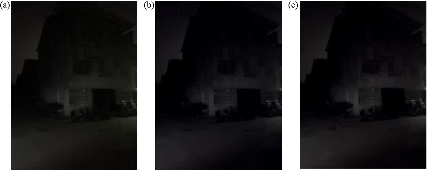
Figure 6: Comparison of denoising effects for low-illumination high-noise urban scenes. (a) Noisy input image; (b) Dual-branch model without FDPL; (c) Dual-branch model with FDPL in this paper.
3.4.3 Efficiency-Accuracy Trade-off
Fig. 7 plots PSNR against model parameters for all competing methods on BSD500 at σ = 12.75. Our model (0.18M, 31.15 dB) occupies a unique position on the Pareto frontier: it achieves the second highest PSNR after RIDNet, yet with only one-fifth of its parameters and 7.4× faster inference. Compared with the ultra-lightweight SwinIR-light, it delivers 0.28 dB higher PSNR while being 33× faster. The plot visually confirms that the proposed network is the most accurate model within a real-time CPU budget, a property that is decisive for practical edge deployment.
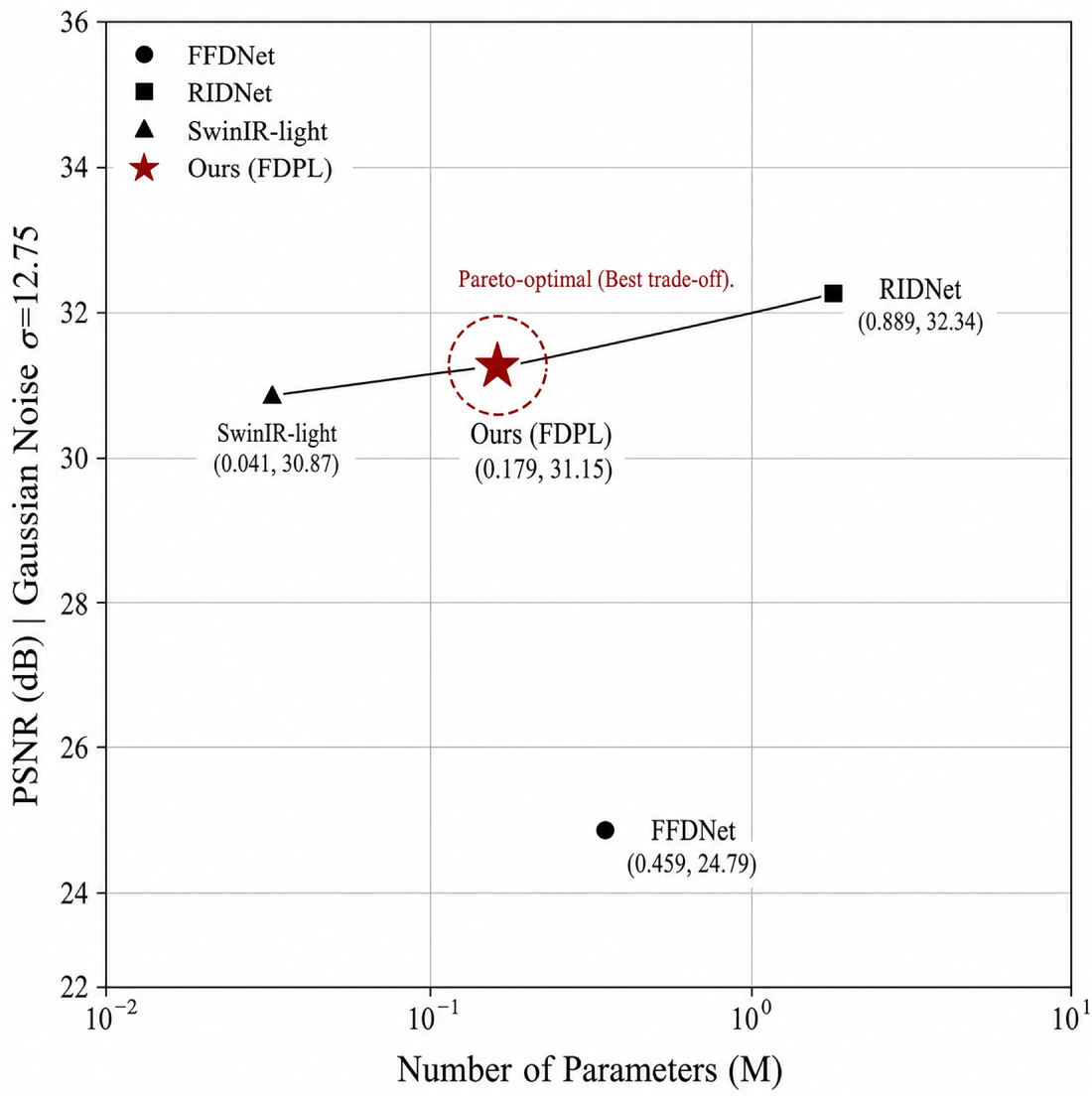
Figure 7: Efficiency–accuracy trade-off on the BSD500 dataset (σ = 12.75). The proposed model occupies a Pareto-optimal position, achieving the highest PSNR among all methods with a real-time CPU budget.
3.4.4 Color Desaturation Limitation
Fig. 8 illustrates the color-flattening phenomenon on a high-saturation snow mountain scene (FUJIFILM X-T5, XF70–300 mm F4–5.6 LM OIS WR, ISO 125, f/5.6, 1/60 s). The original input (Fig. 8a) exhibits strong warm-cool contrast and vivid natural colors. After denoising (Fig. 8b), the warm golden tones are noticeably subdued, the warm-cool contrast weakens, and the overall saturation drops. This limitation stems from the luminance-centric nature of the loss functions and the uniform processing of RGB channels, as analyzed in the Discussion. It points to a clear direction for future improvement, such as color-space decoupling and perceptual color-fidelity losses. A detailed analysis of the root causes is provided in the Discussion section.
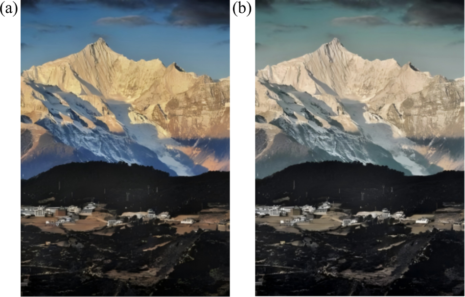
Figure 8: Denoising limitation visualization on high-saturation natural scenes. (a) Input image with high saturation and strong light-dark contrast; (b) Dual-branch model with FDPL in this paper.
4.1 Principal Contributions and FDPL Effectiveness
The proposed model delivers strong multi-dimensional advantages that are consistently validated by the experimental results. By integrating a specialized dual-branch architecture with frequency-domain constraints, it successfully balances the competing goals of noise suppression and detail preservation, directly addressing the over-smoothing problem that has long plagued lightweight denoising models. The low-frequency branch, built with four RRDB modules, focuses on removing Gaussian noise and reconstructing a clean image base, while the high-frequency branch, composed of two RCAB modules, uses channel attention to recover edges and fine textures. This explicit task decoupling is the primary reason behind the model’s solid performance gains: on BSD68, ours (w/FDPL) reaches 31.37 dB PSNR, surpassing DnCNN by 5.28 dB and IRCNN by 5.31 dB. The FDPL loss alone contributes an additional 0.37–0.69 dB across BSD68, CBSD68, and Urban100, confirming its effectiveness in preserving frequency-domain details that conventional spatial losses tend to smooth away. As demonstrated by the spatial error maps and spectral analysis in Fig. 5, the FDPL-equipped model consistently exhibits lower reconstruction error and retains more high-frequency energy, confirming that the proposed frequency-domain loss effectively counteracts the low-pass filtering tendency inherent in MSE-driven optimization.
4.2 Ablation Validation of Architectural Choices
The ablation study provides a complete validation chain for every architectural choice. Swapping the modules between the two branches (RCAB for the low-frequency path, RRDB for the high-frequency path) yields performance that is at best equal to and often slightly worse than the original design (e.g., 31.16 vs. 31.37 dB on BSD68). This demonstrates that the default pairing is the most effective among the configurations we tested, consistent with the characteristics of each module. The plain convolution variant, which strips all specialized mechanisms, suffers a clear PSNR drop on BSD68 and CBSD68, yet paradoxically achieves a higher PSNR on Urban100 (30.16 vs. 29.80 dB). As discussed in Section 3.3.2, this discrepancy is a textbook case of dataset-specific overfitting: the repetitive urban textures are easily memorized by the simple convolution stack, but this capacity does not transfer to diverse natural scenes. In contrast, the proposed model learns generalizable features and continues improving throughout all 50 training epochs. These results underscore that the residual connections, dense connectivity, and channel attention not only boost performance but also act as powerful regularizers against overfitting, a phenomenon consistent with the regularizing effects of deep architectural components widely surveyed in the literature [26].
The brightness-aware MSE loss further strengthens the model’s practicality. By assigning a 1.5× weight to pixels whose luminance exceeds 0.6 (computed via ITU-R BT.601), the model is explicitly encouraged to restore details in bright regions that are often lost by uniform loss functions. This design proves beneficial in scenarios with strong illumination, such as outdoor surveillance, drone-mounted cameras, and medical imaging under brightfield microscopy, where highlight fidelity is crucial for interpretability.
4.3 Efficiency–Accuracy Trade-off and Engineering Implications
The comparison with state-of-the-art lightweight models on BSD500 (Table 3) places our method on a highly favorable position on the Pareto frontier. With 0.18M parameters—five times fewer than RIDNet—and a per-patch CPU inference time of 3.29 ms, our model is 7.4× faster than RIDNet while closing the PSNR gap to only 1.19 dB at σ = 12.75. Against the ultra-lightweight SwinIR-light, it achieves 0.28 dB higher PSNR and runs 33× faster. At σ = 25, the performance remains competitive (27.57 vs. 27.61 dB for SwinIR-light), and the throughput advantage is preserved. These numbers demonstrate that the proposed network is neither the absolute best in PSNR nor the smallest in parameters, but it uniquely achieves the strongest denoising accuracy within a real-time CPU budget—a property of paramount importance for edge-AI applications where both latency and fidelity are hard constraints. The reason behind this favorable balance lies in the dual-branch design, which uses the minimal necessary capacity for high-frequency recovery while dedicating most of the parameters to stable noise suppression, all of which is further enhanced by the FDPL, following efficient architecture design guidelines [27].
This Pareto-optimal position is not merely a numerical advantage but has direct engineering implications: the model’s combination of real-time throughput, low memory footprint, and competitive fidelity removes the traditional barriers to deploying CNN-based denoising on resource-constrained hardware such as smartphones, surveillance cameras, and embedded medical devices. Moreover, because the current evaluation is limited to a single consumer-grade SoC, comprehensive cross-platform benchmarking on ARM CPUs, mobile Neural Processing Units (NPUs), and micro-controllers represents a natural direction for future work, moving the method from algorithmic feasibility to large-scale real-world deployment.
4.4 Limitations in Color Fidelity
Despite its strong overall performance, the model exhibits a subtle but consistent tendency toward color desaturation when processing high-contrast, high-saturation natural scenes (Fig. 8). The root causes are threefold. First, the multi-loss strategy contains no dedicated color-fidelity term: the brightness-aware MSE operates on a derived luma channel, the FDPL penalizes only the amplitude spectrum of the full RGB signal, and the VGG-19 perceptual loss captures semantic structure without explicit chromatic supervision. Second, because the same convolutional kernels are applied uniformly to all three RGB channels, the low-frequency chrominance components that encode smooth color gradations are inevitably attenuated by the denoising process. Third, the quantitative metrics used for training and validation—PSNR and SSIM—are luminance-dominant by nature and provide no feedback on color fidelity. This limitation, however, suggests a clear roadmap for future improvement. Decoupling luminance and chrominance processing by transforming the input into a perceptual color space such as YCbCr (Luminance-Chrominance), Lab (CIE L*a*b*), or YUV (Luminance-Chrominance), and designing separate loss terms for chromatic channels, would likely mitigate the desaturation effect. Incorporating a perceptual color-fidelity loss and adding color-aware metrics to the validation cycle could further guide the network toward more faithful color reproduction. These extensions are part of our planned future work, with the aim of evolving the current model into an integrated image restoration framework that jointly optimizes spatial, frequency, and color dimensions.
This paper presented a lightweight dual-branch CNN denoising network driven by a novel Frequency Domain Perception Loss (FDPL). The architecture explicitly separates low-frequency noise suppression, realized by four RRDB modules, from high-frequency detail recovery, handled by two lightweight RCAB modules. A composite loss function integrates a brightness-aware MSE, a VGG-19 perceptual loss, and the FDPL, which leverages a circular frequency-domain mask with a dynamic warm-up schedule to force the model to retain high-frequency details that are otherwise discarded by traditional losses.
Extensive experiments on BSD68, CBSD68, and Urban100 demonstrate the effectiveness of the proposed design. The full model achieves a PSNR of 31.37 dB on BSD68, outperforming DnCNN by 5.28 dB and IRCNN by 5.31 dB. The FDPL contributes a consistent PSNR gain of 0.37–0.69 dB across all three datasets. When compared against recent state-of-the-art lightweight models—FFDNet, RIDNet, and SwinIR-light—on the BSD500 benchmark under both low (σ = 12.75) and moderate (σ = 25) noise levels, our model demonstrates a compelling efficiency–accuracy trade-off. At σ = 12.75, it reaches 31.15 dB with only 0.18M parameters, closely approaching RIDNet’s 32.34 dB while being 5× smaller and 7.4× faster, and surpassing SwinIR-light by 0.28 dB with a 33× speed advantage. At σ = 25, it achieves 27.57 dB, on par with SwinIR-light while maintaining its real-time throughput.
Ablation studies further validate every component: removing FDPL results in a consistent PSNR drop; swapping the module assignments between branches leads to sub-optimal performance; and replacing RRDB/RCAB with plain convolution layers reveals overfitting on urban textures while proving the necessity of the specialized designs for generalization. The plain convolution variant’s abnormal gain on Urban100 is comprehensively analyzed and attributed to dataset-specific pattern memorization, reinforcing the importance of evaluating denoising methods on diverse benchmarks.
With only 0.18M parameters and a CPU inference time of 3.29 ms per 64 × 64 patch, the model occupies a unique position on the Pareto frontier of accuracy vs. efficiency. It is readily deployable on resource-constrained edge devices for real-time applications such as mobile imaging, surveillance, and on-device preprocessing. The fixed training configuration ensures full reproducibility, providing a solid baseline for future research.
Future work will pursue three directions. First, we will extend the model to handle real-world noise types through more diverse training data and noise-adaptive mechanisms. Second, the observed color-flattening limitation will be addressed by introducing color-space decoupling strategies and perceptual color-fidelity losses. Third, the proposed dual-branch architecture and FDPL loss can be generalized to other low-level vision tasks, such as image deblurring and joint restoration, where the explicit frequency-domain constraint is expected to bring similar benefits.
Acknowledgement: The authors would like to express sincere gratitude to Dr. Guangming Wang, Research Associate at the University of Cambridge, for his valuable academic guidance, professional course teaching on Computer Vision in Robotics, and constructive support throughout the thesis defense and research presentation process.
Funding Statement: The authors received no specific funding for this study.
Author Contributions: Validation, Yixuan Chen; formal analysis, Yixuan Chen; investigation, Yixuan Chen; data curation, Yixuan Chen; writing—original draft preparation, Yixuan Chen; writing—review and editing, Yixuan Chen and Yufeng Qin; visualization, Yixuan Chen; project administration, Yixuan Chen; supervision, Yufeng Qin. All authors reviewed and approved the final version of the manuscript.
Availability of Data and Materials: The data and code that support the findings of this study are available from the first author (Yixuan Chen) upon reasonable request. During the preparation of this work, the authors used ChatGPT (image generation feature, OpenAI) to polish the visual layout of Fig. 1. After using this tool, the authors reviewed and edited the content as needed and take full responsibility for the content of the publication.
Ethics Approval: This study does not involve human participants, animals, or sensitive personal data. All experiments are conducted on publicly available benchmark datasets or synthetic data. Therefore, no ethical approval or institutional review board (IRB) consent is required for this work.
Conflicts of Interest: The authors declare no conflicts of interest.
Abbreviations
The following abbreviations are used in this manuscript:
| CNN | Convolutional Neural Network |
| BN | Batch Normalization |
| DnCNN | Denoising Convolutional Neural Network |
| FDPL | Frequency Domain Perception Loss |
| FFT | Fast Fourier Transform |
| IRCNN | Image Restoration Convolutional Neural Network |
| MSE | Mean Squared Error |
| PSNR | Peak Signal-to-Noise Ratio |
| RCAB | Residual Channel Attention Block |
| ReLU | Rectified Linear Unit |
| RRDB | Residual-in-Residual Dense Block |
| RGB | Red Green Blue |
| SSIM | Structural Similarity Index Measure |
| VGG19 | Visual Geometry Group 19-Layer Convolutional Neural Network |
| YCbCr | Luminance-Chrominance Color Space |
| YUV | Luminance-Chrominance Color Space |
| BM3D | Block-Matching and 3D Filtering |
| ESRGAN | Enhanced Super-Resolution Generative Adversarial Network |
| LeakyReLU | Leaky Rectified Linear Unit |
| ITU-R | International Telecommunication Union Radiocommunication Sector |
| AWGN | Additive White Gaussian Noise |
| AdamW | Adaptive Moment Estimation with Decoupled Weight Decay |
| Adam | Adaptive Moment Estimation |
| FFDNet | Fast and Flexible Denoising Network |
| RIDNet | Real Image Denoising Network |
| SwinIR | Swin Transformer for Image Restoration |
| MAE | Mean Absolute Error |
| SoC | System on Chip |
| MPS | Metal Performance Shaders |
| IRB | Institutional Review Board |
| CPU | Central Processing Unit |
| GPU | Graphics Processing Unit |
| NPU | Neural Processing Unit |
| Lab | CIE L*a*b* |
| VGG | Visual Geometry Group |
| ISO | International Organization for Standardization |
References
1. Buades A, Coll B, Morel JM. A review of image denoising algorithms, with a new one. Multiscale Model Simul. 2005;4(2):490–530. doi:10.1137/040616024. [Google Scholar] [CrossRef]
2. Dabov K, Foi A, Katkovnik V, Egiazarian K. Image denoising by sparse 3-D transform-domain collaborative filtering. IEEE Trans Image Process. 2007;16(8):2080–95. doi:10.1109/TIP.2007.901238. [Google Scholar] [CrossRef]
3. LeCun Y, Bengio Y, Hinton G. Deep learning. Nature. 2015;521(7553):436–44. doi:10.1038/nature14539. [Google Scholar] [CrossRef]
4. Zhang K, Zuo W, Chen Y, Meng D, Zhang L. Beyond a Gaussian denoiser: Residual learning of deep CNN for image denoising. IEEE Trans Image Process. 2017;26(7):3142–55. doi:10.1109/TIP.2017.2662206. [Google Scholar] [CrossRef]
5. Zhang K, Zuo W, Gu S, Zhang L. Learning deep CNN denoiser prior for image restoration. In: Proceedings of the 2017 IEEE Conference on Computer Vision and Pattern Recognition (CVPR); 2017 July 21–26; Honolulu, HI, USA: IEEE; 2017. p. 2808–17. doi:10.1109/CVPR.2017.300. [Google Scholar] [CrossRef]
6. Krizhevsky A, Sutskever I, Hinton GE. ImageNet classification with deep convolutional neural networks. Commun ACM. 2017;60(6):84–90. doi:10.1145/3065386. [Google Scholar] [CrossRef]
7. Huang C, Yang Y, He Y. Salt-and-pepper denoising based on lightweight convolutional neural networks for flexible AMOLED. IET Image Process. 2025;19(1):e13307. doi:10.1049/ipr2.13307. [Google Scholar] [CrossRef]
8. He R, Li X, Wu J. LEESDFormer: A lightweight unsupervised CNN-Transformer-based curve estimation network for low-light image enhancement, exposure suppression, and denoising. Neural Netw. 2025;190:107764. doi:10.1016/j.neunet.2025.107764. [Google Scholar] [CrossRef]
9. Wang X, Tang Y, Yao C, Gao Y, Chen Y. DuINet: a dual-branch network with information exchange and perceptual loss for enhanced image denoising. Digit Signal Process. 2025;156:104835. doi:10.1016/j.dsp.2024.104835. [Google Scholar] [CrossRef]
10. Liu S, Cao L, Zhang Y, Li Y. DBFE-Net: a dual-branch feature extraction network for Gaussian blind denoising. Displays. 2025;90(8):103108. doi:10.1016/j.displa.2025.103108. [Google Scholar] [CrossRef]
11. Yang J, Wright J, Huang TS, Ma Y. Image super-resolution via sparse representation. IEEE Trans Image Process. 2010;19(11):2861–73. doi:10.1109/TIP.2010.2050625. [Google Scholar] [CrossRef]
12. Wang X, Yu K, Wu S, Gu J, Liu Y, Dong C, et al. ESRGAN: Enhanced super-resolution generative adversarial networks. In: Proceedings of the European Conference on Computer Vision (ECCV) Workshops; 2018 Sep 8–14; Munich, Germany. p. 63–79. doi:10.1007/978-3-030-11021-5_5. [Google Scholar] [CrossRef]
13. Hu Y, Li J, Huang Y, Gao X. Channel-wise and spatial feature modulation network for single image super-resolution. IEEE Trans Circuits Syst Video Technol. 2020;30(11):3911–27. doi:10.1109/TCSVT.2019.2915238. [Google Scholar] [CrossRef]
14. Johnson J, Alahi A, Li FF. Perceptual losses for real-time style transfer and super-resolution. In: Proceedings of the European Conference on Computer Vision (ECCV); 2016 Oct 8–16; Amsterdam, The Netherlands. p. 694–711. doi:10.1007/978-3-319-46475-6_43. [Google Scholar] [CrossRef]
15. Tian C, Fei L, Zheng W, Xu Y, Zuo W, Lin CW. Deep learning on image denoising: An overview. Neural Netw. 2020;131(11):251–75. doi:10.1016/j.neunet.2020.07.025. [Google Scholar] [CrossRef]
16. Jiang L, Dai B, Wu W, Loy CC. Focal frequency loss for image reconstruction and synthesis. In: Proceedings of the IEEE/CVF International Conference on Computer Vision (ICCV); 2021 Oct 10–17; Montreal, QC, Canada. p. 13899–909. doi:10.1109/ICCV48922.2021.01366. [Google Scholar] [CrossRef]
17. Hu J, Wang Z. A novel CNN architecture for image restoration with implicit frequency selection. Connect Sci. 2025;37(1):2465448. doi:10.1080/09540091.2025.2465448. [Google Scholar] [CrossRef]
18. Zhou TW, Zhao XL, Wu WH, Wang JL, Luo YS. Frequency-aware implicit neural representation for multi-dimensional data recovery. IEEE Trans Circuits Syst Video Technol. 2025;35(11):10862–74. doi:10.1109/TCSVT.2025.3575475. [Google Scholar] [CrossRef]
19. Arbeláez P, Maire M, Fowlkes C, Malik J. Contour detection and hierarchical image segmentation. IEEE Trans Pattern Anal Mach Intell. 2011;33(5):898–916. doi:10.1109/TPAMI.2010.161. [Google Scholar] [CrossRef]
20. Huang JB, Singh A, Ahuja N. Single image super-resolution from transformed self-exemplars. In: Proceedings of the IEEE Conference on Computer Vision and Pattern Recognition (CVPR); 2015 Jun 7–12; Boston, MA, USA. p. 5197–206. doi:10.1109/CVPR.2015.7299156. [Google Scholar] [CrossRef]
21. Wang Z, Bovik AC, Sheikh HR, Simoncelli EP. Image quality assessment: From error visibility to structural similarity. IEEE Trans Image Process. 2004;13(4):600–12. doi:10.1109/tip.2003.819861. [Google Scholar] [CrossRef]
22. Mittal A, Moorthy AK, Bovik AC. No-reference image quality assessment in the spatial domain. IEEE Trans Image Phrocess. 2012;21(12):4695–708. doi:10.1109/TIP.2012.2214050. [Google Scholar] [CrossRef]
23. Zhang K, Zuo W, Zhang L. FFDNet: Toward a fast and flexible solution for CNN-based image denoising. IEEE Trans Image Process. 2018;27(9):4608–22. doi:10.1109/TIP.2018.2839891. [Google Scholar] [CrossRef]
24. Anwar S, Barnes N. Real image denoising with feature attention. In: Proceedings of the IEEE/CVF International Conference on Computer Vision (ICCV); 2019 Oct 27–Nov 2; Seoul, Republic of Korea. p. 3155–64. doi:10.1109/ICCV.2019.00325. [Google Scholar] [CrossRef]
25. Liang J, Cao J, Sun G, Zhang K, Van Gool L, Timofte R. SwinIR: image restoration using swin transformer. In: Proceedings of the IEEE/CVF International Conference on Computer Vision Workshops (ICCVW); 2021 Oct 11–17; Montreal, BC, Canada. p. 1833–44. doi:10.1109/ICCVW54120.2021.00210. [Google Scholar] [CrossRef]
26. Li Z, Liu F, Yang W, Peng S, Zhou J. A survey of convolutional neural networks: Analysis, applications, and prospects. IEEE Trans Neural Netw Learn Syst. 2022;33(12):6999–7019. doi:10.1109/TNNLS.2021.3084827. [Google Scholar] [CrossRef]
27. Wang CH, Huang KY, Yao Y, Chen JC, Shuai HH, Cheng WH. Lightweight deep learning: An overview. IEEE Consum Electron Mag. 2024;13(4):51–64. doi:10.1109/MCE.2022.3181759. [Google Scholar] [CrossRef]
Cite This Article
 Copyright © 2026 The Author(s). Published by Tech Science Press.
This work is licensed under a Creative Commons Attribution 4.0 International License , which permits unrestricted use, distribution, and reproduction in any medium, provided the original work is properly cited.
 Downloads
 Citation Tools
