Physics-Informed Neural Networks for Hail-Impact Dynamics of Photovoltaic Panels: Multi-Condition Forward Modeling and Inverse Identification of Contact Stiffness

1  Introduction

The global installed capacity of photovoltaic (PV) systems has surpassed one terawatt [1], yet the structural resilience of PV laminates against severe weather events, such as hailstorms, remains a critical concern for long-term energy yield and asset valuation. Experimental hail-impact studies have shown that the contact between a hail particle and a PV glass panel generates strongly nonlinear restoring forces. These forces depend largely on the compliance of the supporting substrate and produce qualitatively distinct indentation, cracking, and delamination patterns.

Researchers demonstrated that the resulting contact dynamics can be represented by a single-degree-of-freedom (SDOF) oscillator [2]. This experimentally grounded model forms the physical basis of the present study. From a design and monitoring standpoint, two complementary tasks arise. First, for a given substrate and hail-speed scenario, the forward impact response must be predicted rapidly enough to permit parametric screening across the range of impact velocities. Second, when sparse vibration measurements are available from an instrumented panel after a hail event, the effective contact stiffness coefficients must be identified from those data, as deviations from baseline values serve as indicators of substrate degradation. Classical time-integration schemes such as the Newmark-β method [3] can address the first task with high accuracy, but every new velocity or parameter set demands a new simulation. The second problem, namely, the inverse identification of multiple nonlinear coefficients from limited data, lies outside the natural scope of traditional forward solvers altogether. These dual limitations motivate the present work.

In recent years, PINNs have emerged as a promising approach to address these challenges. PINNs belong to the broader class of physics-informed machine learning methods that incorporate governing equations and initial/boundary conditions directly into the training process of neural networks [4–11]. By embedding known physical laws into the loss function, PINNs are capable of learning solutions to differential equations with minimal or even no labeled data.

A particular focus within the mechanics community has been the application of PINNs to dynamic simulations, i.e., time-dependent problems such as vibrations, wave propagation, and structural responses to external loads. In the standard PINN formulation, time is treated as an additional input variable, allowing the neural network to learn the complete space-time solution of a dynamical system [12–14]. Recent studies have further extended PINNs to contact mechanics. For instance, Sahin et al. [15] proposed a mixed-variable PINN with output transformations to enforce boundary conditions and incorporated Karush-Kuhn-Tucker (KKT) contact constraints through a Fischer–Burmeister formulation, demonstrating accurate forward, inverse, and surrogate modeling for the Hertzian contact problem. More broadly, PINNs and their variants have been applied to a wide spectrum of nonlinear dynamical systems [16–18]. For example, Zhu et al. [19] employed PINNs for hydrodynamic analysis to model vortex-induced vibrations, while Shaikh et al. [20] developed a PINN-based inverse framework to identify forcing functions in Duffing oscillators, achieving high accuracy in dynamic load identification.

A well-documented challenge for PINNs applied to dynamical systems is spectral bias: neural networks trained with gradient descent tend to learn low-frequency components of the target function more readily than high-frequency features [21]. This tendency is rooted in the spectral properties of the neural tangent kernel [22] and has been shown to hinder the accurate learning of solutions containing sharp gradients or rapid oscillations precisely the features present in stiff impact dynamics. Several mitigation strategies have been proposed, including curriculum learning [23], multiscale Fourier feature mappings [24], Kronecker architectures [25], and modal-informed network design [26]. While these approaches show promising improvements for specific problem classes, many require problem-specific tuning and labeled data, and their integration can complicate the unified forward inverse workflow that is a key advantage of the standard PINN framework [27]. In the present work, spectral bias is mitigated through careful nondimensionalization of all variables and coefficients (Section 2.3.1), which brings the polynomial stiffness terms spanning up to fifteen orders of magnitude in their dimensional form into a numerically balanced range. This practical strategy, combined with the multi-condition training approach described in Section 2.4, proves sufficient for the systems considered here without requiring specialized network architectures.

Beyond forward simulation, PINNs have attracted increasing interest for inverse problems in structural and nonlinear dynamics, particularly for identifying unknown system parameters from measured response data. Lai et al. [28] combined physics-informed Neural ODEs with sparse regression to identify structural models from vibration measurements, while Haghighat et al. [29] developed a multi-network PINN architecture for material-parameter inversion in solid mechanics. Linka et al. [30] incorporated Bayesian inference within the PINN framework to quantify parametric uncertainty in nonlinear oscillators under sparse and noisy data. More recently, Zhai et al. [31] proposed a Runge-Kutta PINN (RK-PINN) that embeds integration cells to enable parameter estimation for nonlinear dynamical systems subjected to external excitations. Raj and Banerjee [32] introduced Fisher-information-guided PINNs with Fourier feature embeddings for real-time parameter identification in digital twins of vibratory systems.

These studies highlight the versatility of physics-informed learning for solving inverse problems. However, to the best of the authors’ knowledge, no existing study has applied physics-informed learning to the specific problem of characterizing contact stiffness in hail-loaded PV laminates, with highly stiff nonlinear equations. This combination of extreme coefficient ranges, stiff dynamics, and the practical need for both rapid forward evaluation and sparse-data inverse identification constitutes an unresolved challenge at the intersection of nonlinear dynamics and structural health monitoring of renewable energy systems.

It is also important to recognize the broader limitations of PINNs reported in the literature. In many cases, training a PINN can be orders of magnitude slower than executing a conventional solver for a single scenario [33], and the models are often more difficult to tune due to their problem-dependent optimization behavior [34]. In terms of forward-simulation accuracy, Grossmann et al. [35] showed that PINNs do not consistently outperform standard finite element methods, reinforcing that they are not yet a replacement for established numerical solvers. Despite growing interest in PINN-based computational mechanics and structural dynamics, there are still gaps in the literature that motivate the present work. First, most PINN formulations for engineering problems train a separate network per initial condition, yielding single-trajectory surrogates that require full retraining for each new loading scenario [4,29]. Second, although parametric PINNs have recently been proposed to embed problem parameters as explicit inputs [36], their application has remained confined to canonical benchmark PDEs, and velocity-conditioned nonlinear impact dynamics have not been addressed. Third, PINN-based contact studies are restricted to static or quasi-static elasticity, while prior PV hail-impact work has demonstrated the decisive role of substrate stiffness on damage yet relies on conventional finite element solvers without inverse-identification capability [2]. The present work closes all three gaps by introducing a velocity-conditioned parametric PINN that learns a multi-speed impact solution map, paired with a physics-informed two-phase inverse algorithm that recovers polynomial contact stiffness coefficients from sparse, noisy measurements across soft, medium, and hard substrate regimes.

In light of the current state of the art, this study focuses on the intersection of PINNs and nonlinear impact mechanics, an area that presents both significant potential and unresolved challenges. The main contributions of the present work are summarized as follows:

1.   Parametric PINN for nonlinear hail-impact dynamics. A forward PINN formulation is developed in which the impact velocity is introduced as an explicit input parameter. This allows a single trained network to represent the transient response over a range of impact conditions, instead of learning only one fixed trajectory. The trained model is further evaluated at unseen impact velocities to assess its interpolation capability and to demonstrate that it learns a velocity-dependent solution map.

2.   Physics-informed inverse PINN framework for parameter estimation. A hybrid inverse-identification strategy is proposed for estimating the effective coefficients of the nonlinear impact model from sparse displacement data from numerical simulation with Gaussian noise. The approach combines physics-informed residual minimization with a least-squares parameter-update step, enabling the recovery of contact stiffness parameters relevant to PV backing-layer degradation assessment without requiring direct indentation-based characterization.

3.   Robust validation across impact regimes, benchmark systems, and noisy observation. The proposed framework is systematically evaluated on six hail-impact configurations, covering soft, medium, and hard stiffness regimes with both undamped and damped responses. In addition, two representative benchmark oscillators, namely the Duffing oscillator and the belt–mass system, are considered. The forward model is tested at unseen impact velocities, while the inverse framework is assessed under noisy displacement and velocity observations to examine its robustness under more realistic measurement conditions.

The remainder of this paper is organized as follows. Section 2 presents the governing equations of the considered nonlinear dynamical systems, along with the proposed PINNs framework. This includes the multi-condition and inverse formulations, and the loss function design. Section 3 focuses on the forward problem, where the capability of the PINN to accurately reproduce system dynamics is assessed for different nonlinear oscillators. It also includes addresses the inverse problem, demonstrating the identification of unknown physical parameters using the proposed hybrid and physics-informed strategies. Section 4 concludes the paper and outlines potential directions for future research.

2  Problem Formulation

In this section, we introduce the analytical models considered in this work, focusing on three representative nonlinear dynamical systems: (i) a single-degree-of-freedom (SDOF) impact oscillator with polynomial restoring forces; (ii) the Duffing oscillator, a classical nonlinear system with cubic stiffness and viscous damping; and (iii) a belt–mass oscillator that combines linear and quadratic damping with cubic stiffness, capturing nonlinear dissipation effects.

These systems allow us to examine the proposed framework across different types of nonlinear behavior, ranging from stiffness-driven impact dynamics to nonlinear resonance and damping-dominated responses. The section also outlines the key components of the methodology, including the multi-condition PINN architecture, the physics-informed inverse formulation, the adopted non-dimensionalization strategy, the design of the loss function, and the Newmark–β scheme used to generate reference solutions.

2.1 Nonlinear Analysis of Single-Degree-of-Freedom Oscillator

The nonlinear single-degree-of-freedom (SDOF) oscillator is derived from Newton’s second law for a lumped mass–spring–damper system with a nonlinear restoring force R(u). Let u(t) denote the displacement of the mass. The general dynamic equilibrium equation can be expressed as follows:

Mu¨(t)+Cu˙(t)+K(u)u(t) = F(t),(1)

where M is the mass, C is the damping, R(u)=K(u)u is the (generally nonlinear) restoring force, and F(t) is an external load. This type of equation arises in a wide range of structural engineering applications [37,38]. For example, the hysteretic response of an inelastic system can be modeled [39] by expressing the restoring force as R(u)=αku+(1−α)kz which is decomposed into an elastic component αku and a hysteretic component, (1−α)kz. Here, 0≤α≤1 is a weighting parameter, k is the constant stiffness, and z represents an internal hysteretic displacement variable. This model reduces to the present formulation when α=1 and K(u)=k. Although the hysteretic component is not explicitly considered in the present formulation, nonlinearity is incorporated through a more general nonlinear stiffness function. This formulation therefore allows the representation of a broad class of nonlinear physical responses encountered in materials and structural systems.

In the present study, the focus is on the unforced (F(t)=0) oscillator and, unless otherwise stated, neglect linear damping in the baseline impact configuration (C=0). The resulting system can be written as follows [2]:

Mu¨(t)+K(u)u(t) = 0.(2)

To emulate impact behavior using a smooth surrogate, the restoring force is modeled with a high-order polynomial that stiffens rapidly as the amplitude increases:

K(u)u(t) = w∗u(t) + A∗u2(t) + B∗u3(t) + C∗u4(t).(3)

Substituting Eq. (3) into Eq. (2) and dividing by M yields the following second-order nonlinear ordinary differential equation:

u¨(t) + ω02u(t) + Au2(t) + Bu3(t) + Cu4(t) = 0.(4)

The coefficients in Eq. (4) are expressed in mass-normalized form in Eq. (5):

ω02 = w∗M,A = A∗M,B = B∗M,C = C∗M.(5)

To investigate the influence of stiffness severity and nonlinearity, three regimes are considered: soft, medium, and hard. These regimes are defined by the coefficients listed in Table 1, which were experimentally determined from indentation tests on substrates made of different materials [2].

These three substrate types are directly relevant to photovoltaic panel construction. In standard PV laminate assemblies, the glass–encapsulant–cell stack is mounted on a backing layer whose compliance governs the contact mechanics during hail impact. The coefficients in Table 1 were determined by Corrado et al. [2] from quasi-static indentation tests on substrates representative of those used in commercial PV modules. The physical system could be observed in Fig. 1. In the experiments, each regime corresponds to a distinct type of substrate. The hard case represents a wooden board, which exhibits the highest stiffness and produces localized indentation with concentrated cracking around the impact point. The medium case corresponds to an alveolar polycarbonate layer, providing moderate compliance and resulting in a broader crack field characterized by both radial and circumferential features. The soft case represents an expanded polystyrene layer, which has the lowest stiffness and leads to widespread deformation accompanied by extended circumferential cracking.

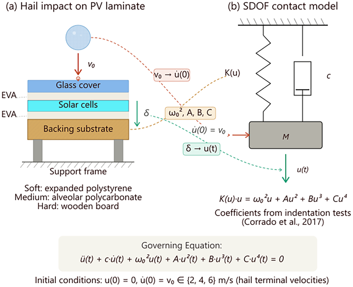
Figure 1: Hail-impact model for photovoltaic laminates. (a) Physical configuration showing the layered laminate and three substrate types of increasing stiffness. (b) Equivalent SDOF oscillator with polynomial contact stiffness.

For compact notation, these cases may equivalently be treated as a parametric family which is represented in Eq. (6):

𝒮:(ω02,A,B,C) ↦ (ω02,κAA,κBB,κCC)(6)

where κA,κB,κC∈{κsoft,κmed,κhard} with κsoft<κmed<κhard.

The baseline initial conditions are adopted from experimental hail-impact tests on photovoltaic panels [2]: u(0)=0.0 m and u˙(0)=6.0 m/s, corresponding to the terminal velocity of a standard 25 mm ice sphere under free fall, consistent with the IEC 61215 hail resistance test protocol. To explore a broader range of hail sizes and impact energies, the multi-condition training extends this to v0∈{2,3,4,6} m/s, covering the terminal velocity range of hailstones with diameters from approximately 10 to 25 mm.

u(0) = 0.0m,u˙(0) = 6.0m/s.(7)

To investigate the stabilizing influence on stiff dynamics, we consider an additional model that incorporates viscous damping. Following a derivation analogous to that for the undamped case, the generalized ODE for the damped system is given by Eq. (8):

u¨(t) + cu˙(t) + ω02u(t) + Au2(t) + Bu3(t) + C4u4(t) = 0,(8)

where the damping coefficient per unit mass c∈{100,1000} [Ns/kgm].

2.2 Benchmark Problems

To demonstrate the generality and portability of the PINN framework beyond impact dynamics, two benchmark nonlinear oscillators with distinct damping and stiffness terms, namely, the Duffing oscillator and the belt-mass oscillator, are considered here. Their formulations and parameters are adopted from the literature [31,40] and shown in Figs. 2 and 3. Herein, the Duffing oscillator represents a single-degree-of-freedom mass–spring system with cubic nonlinear stiffness, commonly used to study nonlinear resonance and amplitude-dependent dynamics. While, the belt–mass system models a mass interacting with a moving belt, where the presence of both linear and quadratic damping captures nonlinear dissipation effects typical of friction-driven systems.

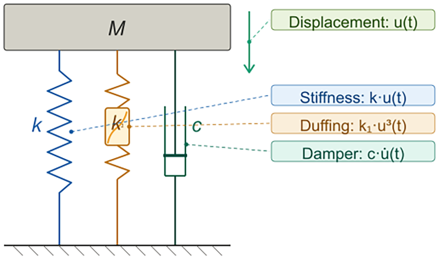
Figure 2: Benchmark System A: Duffing oscillator.

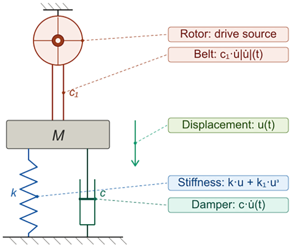
Figure 3: Benchmark System B: Belt–mass system.

2.2.1 Duffing Oscillator

The nonlinear governing equation for the damped vibration of the Duffing oscillator reads:

mu¨(t) + cu˙(t) + ku(t) + k1u3(t) = 0.(9)

The following parameters expressed in international system and adopted from [31,40]:

m = 1.0,c = 50.0,k = 1.0×104,k1 = 2.0×106,(10)

and the initial conditions

u(0) = 1.0,u˙(0) = 0.0.(11)

are adopted for the analysis.

2.2.2 Belt–Mass Oscillator with Linear-Quadratic Damping and Cubic Stiffness

As a second benchmark problem, the belt–mass oscillator with linear–quadratic damping and cubic stiffness is considered, whose governing equation is given in Eq. (12) as:

mu¨(t) + cu˙(t) + c1u˙(t)|u˙(t)| + ku(t) + k1u3(t) = 0.(12)

The following parameters expressed in international system and are adopted from [31,40]:

m = 15.45,c = 600,c1 = 450,k = 3.56×105,k1 = 6.85×107,(13)

and the initial conditions

u(0) = 0.01,u˙(0) = 0.0(14)

are adopted for the analysis. This model captures rapid energy dissipation through the c1u˙|u˙| term and exhibits strong stiffness nonlinearity, making it representative of belt-driven or friction-influenced mechanisms.

2.3 Physics-Informed Neural Networks

PINNs provide a framework for approximating the solution of differential equations by embedding the governing physics directly into the training of a neural network. In this work, a feed-forward neural network uθ(t) is used to represent the system response, where the network parameters θ are optimized such that the predicted solution satisfies both the governing equation and the prescribed initial conditions. The required time derivatives are computed using automatic differentiation, allowing the residual of the differential equation to be enforced within the loss function. This formulation enables the network to learn physically consistent solutions without relying solely on labeled data, and serves as the foundation for both the forward and inverse modeling strategies developed in this study.

Fig. 4 illustrates the overall PINN framework adopted in this work. The neural network takes time t as input and predicts the system response u(t). Automatic differentiation is then used to compute the required time derivatives. The training is guided by a combined loss function that incorporates the physics residual, data mismatch, and initial condition constraints. The resulting gradients are used to update the network parameters, which ensures that the learned solution remains consistent with both the observed data and the underlying physical model.

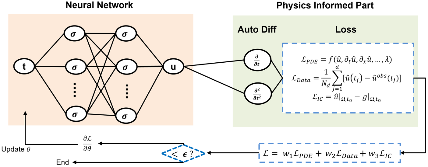
Figure 4: Schematic of the physics-informed neural network (PINN) framework. The neural network maps time to displacement, while automatic differentiation provides the required derivatives to enforce the governing equation. The training is guided by a combined loss incorporating physics, data, and initial condition constraints.

The governing equation for a generic nonlinear oscillator can be written as in Eq. (15):

u¨(t)+𝒩[u(t),u˙(t)]=0.(15)

Within the PINN framework, the network prediction uθ(t) is substituted into the governing equation to define the residual

r(t;θ)=u¨θ(t)+𝒩[uθ(t),u˙θ(t)],(16)

which is minimized at collocation points t∈[0,T] during training.

Loss Function

Direct training on dimensional variables proved to be unstable due to large differences in the magnitudes of the coefficients. To improve numerical conditioning, all variables and coefficients are therefore expressed in nondimensional form shown below:

u=u0u^,t=t0t^,(17)

In Eq. (17), u^ and t^ denote the dimensionless displacement and time variables, respectively, obtained by scaling the physical variables as u=u0u^ and t=t0t^, where u0 and t0 are characteristic reference scales. Substituting these expressions yields the following scaled coefficients:

A∗=Au0t02,B∗=Bu02t02,C∗=C4u03t02,ω0∗=ω0t0.(18)

The total loss (ℒ) of the PINN in the present study is the sum of the physics, initial condition (IC), and data loss terms, expressed in Eq. (19):

ℒ=ℒphys+ℒIC+λdataℒdata.(19)

For the specific systems considered in this work, the residual r(t;θ) takes the form defined in Eq. (16) with the corresponding nonlinear operator 𝒩[⋅]. The physics loss (ℒphys) is defined as the mean squared residual of the governing equation:

ℒphys=1Nc∑i=1Ncr2(ti;θ),(20)

evaluated at collocation points {ti}i=1Nc.

The IC loss (ℒIC) is expressed in Eq. (21) as:

ℒIC=(uθ(0)−u0∗)2+(u˙θ(0)−v0∗)2.(21)

The data loss term (ℒdata) is used in hybrid settings, such as the Duffing oscillator and the belt–mass oscillator, and is defined in Eq. (22) as:

ℒdata=1Nd∑j=1Nd[uθ(tj)−uref(tj)]2,(22)

which is restricted to the early transient phase. Furthermore, the variable λdata in Eq. (19) serves as a controlling weight.

For the current problem, a PINN architecture with 3 hidden layers and 64 neurons was chosen. To justify the selected PINN architecture, a width-and-depth sensitivity analysis was performed for the soft-undamped case at 6.0 m/s initial velocity. Networks with widths of 32, 64, and 128 neurons and depths of 2, 3, and 4 hidden layers were compared for 3000 training epochs. The results shown in the Fig. 5, indicate that two-layer networks were less accurate, while four-layer networks increased the computational cost and did not consistently improve the prediction accuracy. The 3 × 128 network achieved the lowest L2 error, whereas the current 3 × 64 network provided a favourable compromise between accuracy and training time. Therefore, the current network architecture was adopted in the present study.

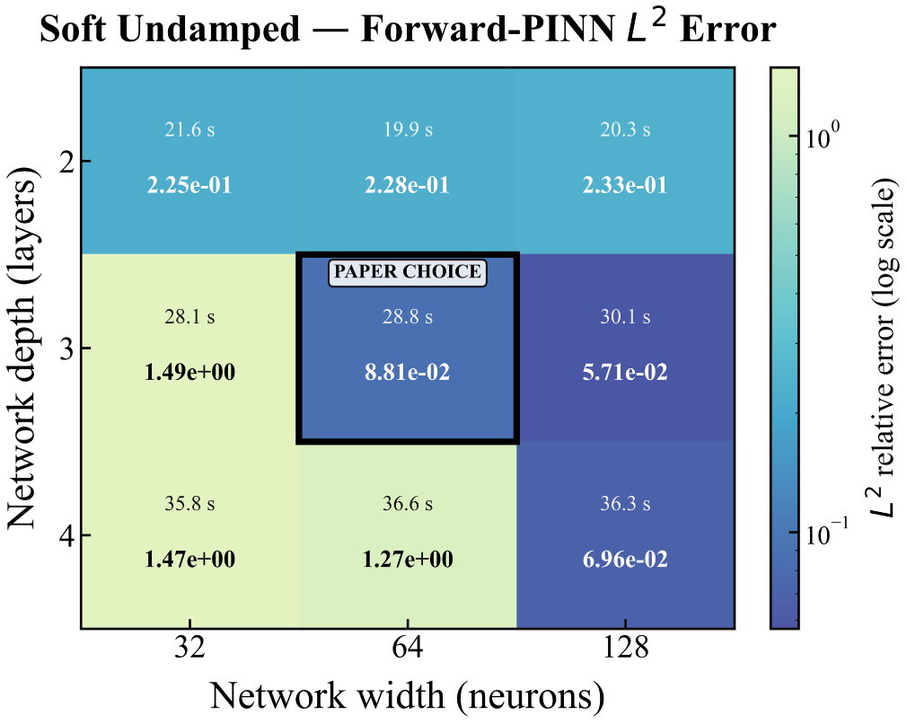
Figure 5: Architecture ablation study for optimal depth and width of the network.

The network is trained using the Adam optimizer with a learning rate of 10−3. In a typical run, Nc=200 collocation points are uniformly sampled in the normalized time domain [0,1], and training is carried out in full-batch mode at each epoch. Since the governing problem considered here is a low-dimensional nonlinear dynamical system, this number of points provides sufficient residual coverage over the complete response interval while keeping the training cost moderate. Uniform sampling was adopted to avoid introducing case-specific bias in the residual evaluation. However, for very stiff impact regimes where the response becomes highly localized in time, adaptive residual-based or importance-weighted collocation could be beneficial by placing more points near the contact-dominated portion of the trajectory. This extension is particularly relevant for future multi-degree-of-freedom or spatially resolved impact models.

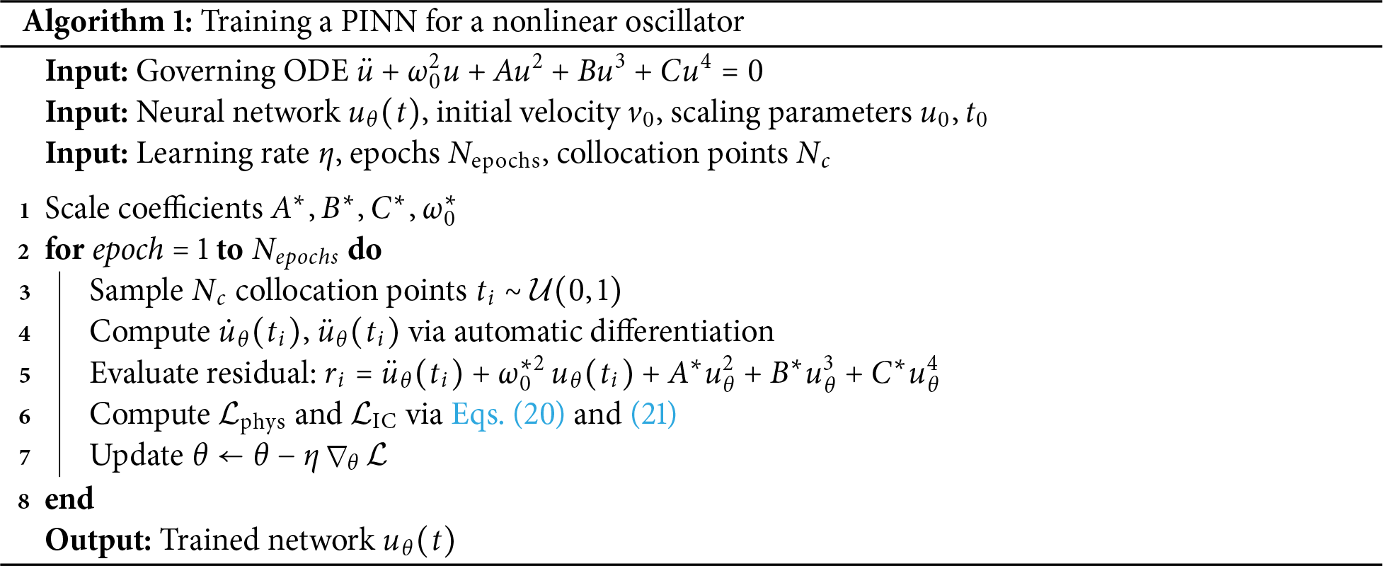
For the baseline impact oscillator, no displacement data are used; the training relies solely on physics residuals and initial conditions. For the benchmark problems, hybrid terms are selectively introduced to incorporate partially supervised data into the loss function. The PINNs training procedure is presented in Algorithm 1. It describes the training of the forward PINNs for a given nonlinear oscillator. The network is trained by minimizing a loss composed of the governing equation residual and initial condition constraints. At each iteration, collocation points are sampled, after which the network prediction and its derivatives are computed via automatic differentiation. Finally the parameters are updated using gradient-based optimization.

2.4 Multi-Condition Forward Training

A key limitation of standard PINN training for ODEs is that the learned model is tied to a single initial condition and therefore lacks predictive capability for other trajectories of the same system. To address this limitation, we augment the network input with the initial velocity v0, enabling the PINN to learn a family of solutions parameterized by the initial state:

u^θ(t^,v0) ≈ u(t;v0),v0∈𝒱,(23)

In Eq. (23), 𝒱={v0(1),v0(2),…,v0(K)} is a discrete set of initial velocities drawn from experimentally relevant values.

During each training epoch, the loss is accumulated over all K initial conditions, such that:

ℒtotal=1K∑k=1K[ℒphys(k)+ℒIC(k)+λdataℒdata(k)],(24)

where in Eq. (24), each component is evaluated along the trajectory corresponding to v0(k). The physics residual ℒphys(k) enforces the governing ODE at collocation points sampled for each initial condition, while ℒdata(k) penalizes discrepancies with sparse reference data obtained from the Newmark solver. By sharing the network weights θ across all initial conditions, the PINN is encouraged to learn the underlying system dynamics rather than overfitting to a single trajectory.

In this study, each impact case is analyzed using four (K=4) initial velocities, i.e., v0∈{2,3,4,6} m/s, representing the range of experimentally relevant hail-impact speeds. The trained model was evaluated at an unseen impact velocity of 5 m/s, which lies within the training range, for all considered cases.

The benchmark systems (Duffing and belt–mass oscillators) are considered with single initial conditions, as their dynamics are already well validated in the existing literature.

2.5 Inverse PINN Formulation for Parameter Estimation

For the inverse problem, the objective is to recover the unknown physical parameters p of the governing ODE from sparse displacement measurements. Rather than relying solely on data fidelity, the governing equation is embedded directly into the training loss through either a weak-form residual (for impact cases) or a strong-form residual (for benchmark cases), thereby constituting a genuinely physics-informed neural network.

A central challenge is that jointly optimizing the network weights and physical parameters through a single composite loss is notoriously ill-conditioned: inaccurate parameter estimates create a spurious physics-loss landscape that corrupts the network’s displacement field, which in turn leads to even poorer parameter estimates in a destructive feedback loop. This issue is addressed through a three-pronged strategy: (i) alternating updates of the network weights and physical parameters so that each subproblem remains well conditioned, (ii) gradient-balanced weighting of the physics loss to prevent the ODE residual from overwhelming the data signal, and (iii) an exponential ramp that gradually introduces the physics loss during training.

Phase 1: Warm-up.

The neural network uθ(τ) is trained for Nw epochs using only the data-fidelity and initial-condition losses as given in Eq. (25):

ℒwarm=λdataℒdata+λICℒIC,(25)

where ℒdata=1Nd∑i=1Nd[(u^i−uiobs)2+(u˙^i−u˙iobs)2] penalizes mismatch in both displacement and velocity, and ℒIC=(u^(0)−u0)2+(u˙^(0)−v0)2 enforces the initial conditions. The physical parameters are held fixed at an initial guess p0=0.5ptrue. This phase establishes a smooth, data-consistent displacement field before the physics loss is introduced.

Phase 2: Alternating optimization with gradient-balanced physics

Training proceeds for Nr rounds, each consisting of a parameter-identification step followed by Na epochs of network refinement:

Step A—Analytical least-squares parameter update

At the beginning of each round-and periodically every L epochs within the round-the physical parameters are updated by solving a linear least-squares problem. Using the current network-predicted displacement u^θ(ti) together with the observed velocity u˙iobs at the Nd measurement points, we construct the design matrix Φ, whose columns are derived from the structural form of the governing equation and is given in Eq. (26):

Φp=−u¨obs,pLS=arg⁡minp‖Φp+u¨obs‖22,(26)

where u¨,obs denotes the acceleration computed from the reference solver at the observation points. and pLS denotes the least-squares estimate of the unknown parameter vector, obtained by minimizing the squared residual of the governing equation in a strong-form sense using the current network prediction and observed data. This strong-form least-squares formulation employs the point-wise ODE residual and remains numerically well conditioned even when the nonlinear displacement columns exhibit strong collinearity (e.g., in overdamped impact cases). The updated parameter estimates are stabilized using an exponential moving average and given in Eq. (27) as:

p←αEMApLS+(1−αEMA)pold,(27)

where αEMA=0.15.

For the impact cases, the design matrix columns are defined as:

Φ=[u˙obs, u^, u^2, u^3, u^4](28)

for the damped system, and

Φ=[u^, u^2, u^3, u^4](29)

for the undamped system, where u^=u^θ(ti). For the belt–mass benchmark problem, an additional quadratic damping term, u˙,obs|u˙,obs|, is included alongside the standard linear damping and stiffness columns in the design matrix.

Step B—Gradient-balanced network refinement

The neural network weights are updated using the Adam optimizer to minimize the composite loss, as mentioned in Eq. (30):

ℒ=λdataℒdata+λICℒIC+λphyseffℒphys,(30)

where the physics loss ℒphys is defined as the mean-squared ODE residual evaluated using the detached (fixed) parameters obtained in Step A and Here, λphyseff denotes the effective weighting coefficient of the physics loss. For the impact cases, the residual is computed in a weak (integral) form via Galerkin projection onto sinusoidal test functions, which avoids the explicit evaluation of u′′ and provides improved robustness for polynomial nonlinearities. For the benchmark cases, the residual is evaluated in strong form using collocation at uniformly spaced interior points.

Crucially, the parameters appearing in ℒphys are detached from the computational graph, so the Adam optimizer updates only the network weights. In this way, the ODE residual serves as a regularizer that guides the network toward physics-consistent trajectories without introducing a direct gradient path to the parameters.

Inverse-Dirichlet gradient balancing

The effective physics weight λphyseff is determined adaptively using the gradient-balancing strategy proposed in [41]:

λphyseff=λ^r(t)s,λ^=α‖∇θℒdata‖‖∇θℒphys‖,(31)

where in Eq. (31), α∈[0.02,0.1] is a case-dependent cap that limits the physics gradient to at most α times the norm of the data gradient. While, λ^ denotes the intermediate (unscaled) physics-loss weighting factor obtained from the ratio of gradient norms, prior to applying the ramp function and safety scaling.

For computational efficiency, the gradient norms are recomputed every 100 epochs; between updates, the most recently computed value of λ^ is reused.

Tracking of best model state

Throughout Phase 2, the model state and parameters corresponding to the lowest relative L2 displacement error are recorded. At the end of training, this best-performing network state is restored, and a final least-squares (LS) parameter update (Eq. (26)) is performed using the restored network. This ensures that the reported parameters are consistent with the displacement field that provides the best fit to the data.

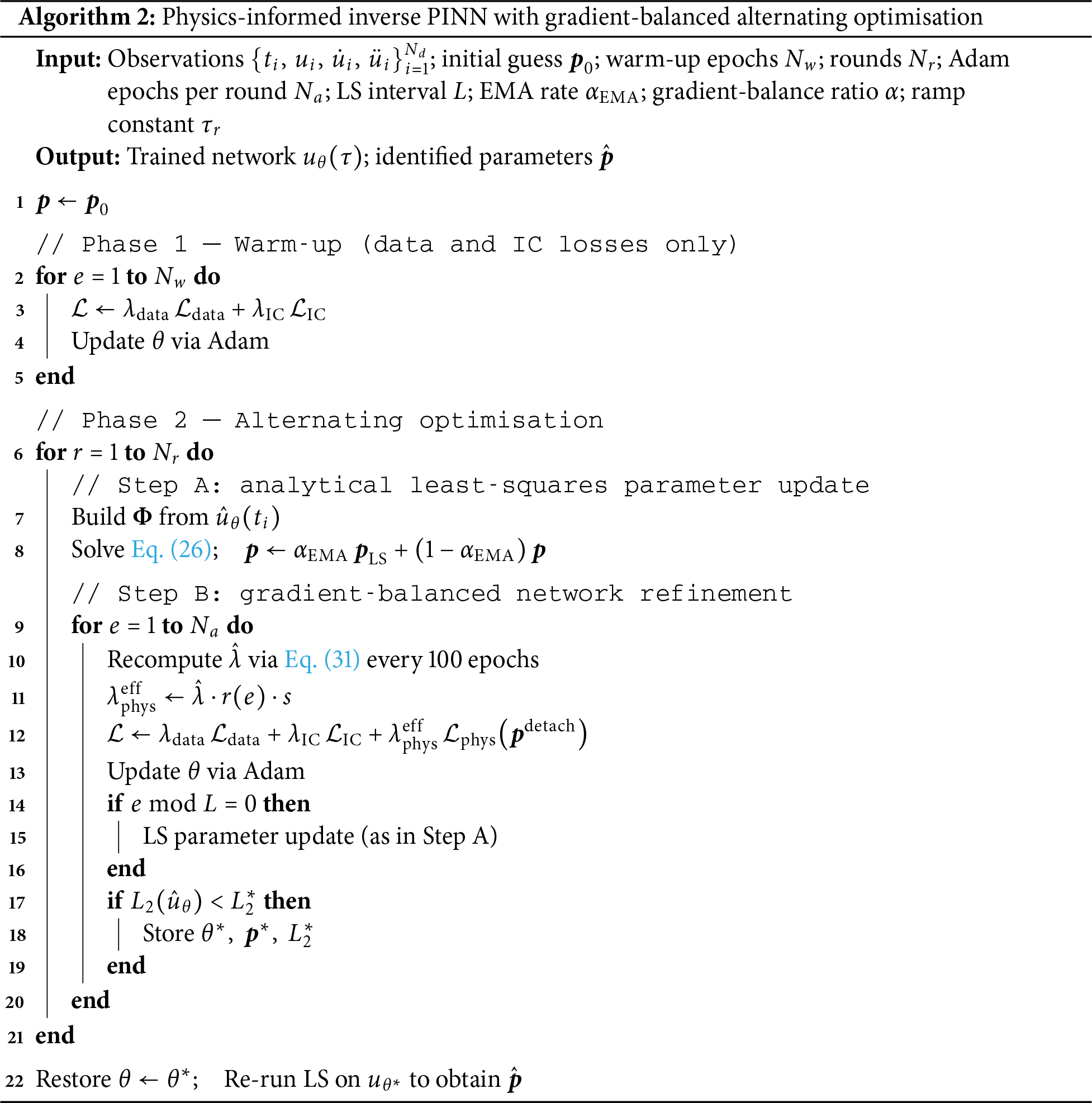
The complete procedure is summarized in Algorithm 2. This algorithm presents the proposed inverse PINN framework. The training proceeds in two stages. First, a short warm-up phase is performed using only data and initial condition losses to obtain a stable initial solution. This is followed by an alternating optimization procedure, where the physical parameters are updated through a least-squares step, and the network is subsequently refined using a gradient-balanced loss that incorporates physics. This decoupled strategy improves stability and robustness in parameter identification.

2.6 Benchmark Numerical Solver: Newmark-β Time Integration Scheme

To benchmark the accuracy of the proposed PINN framework, reference solutions are computed using the classical Newmark family of time-integration schemes, which are widely employed in structural dynamics. A general nonlinear oscillator can be represented in Eq. (32) as:

Mu¨(t)+Cu˙(t)+R(u(t))=0,(32)

with restoring force R(u) (potentially nonlinear), the Newmark scheme discretizes displacement and velocity over uniform time steps Δt as follows:

un+1=un+Δtu˙n+Δt2(12−β)u¨n+βΔt2u¨n+1,(33a)

u˙n+1=u˙n+Δt(1−γ)u¨n+γΔtu¨n+1,(33b)

where β and γ are scheme parameters in Eq. (33). Choosing γ=1/2 and β=1/4 yields the constant-average-acceleration method, which is second-order accurate and unconditionally stable for linear problems. The implementation of the classical Newmark method is summarized in Algorithm 3. In this algorithm we outlined the Newmark–β method used to generate reference solutions. The method advances the solution in time using a predictor-corrector approach combined with Newton iterations to handle nonlinearities. It also provides reliable benchmark data for training and validation.

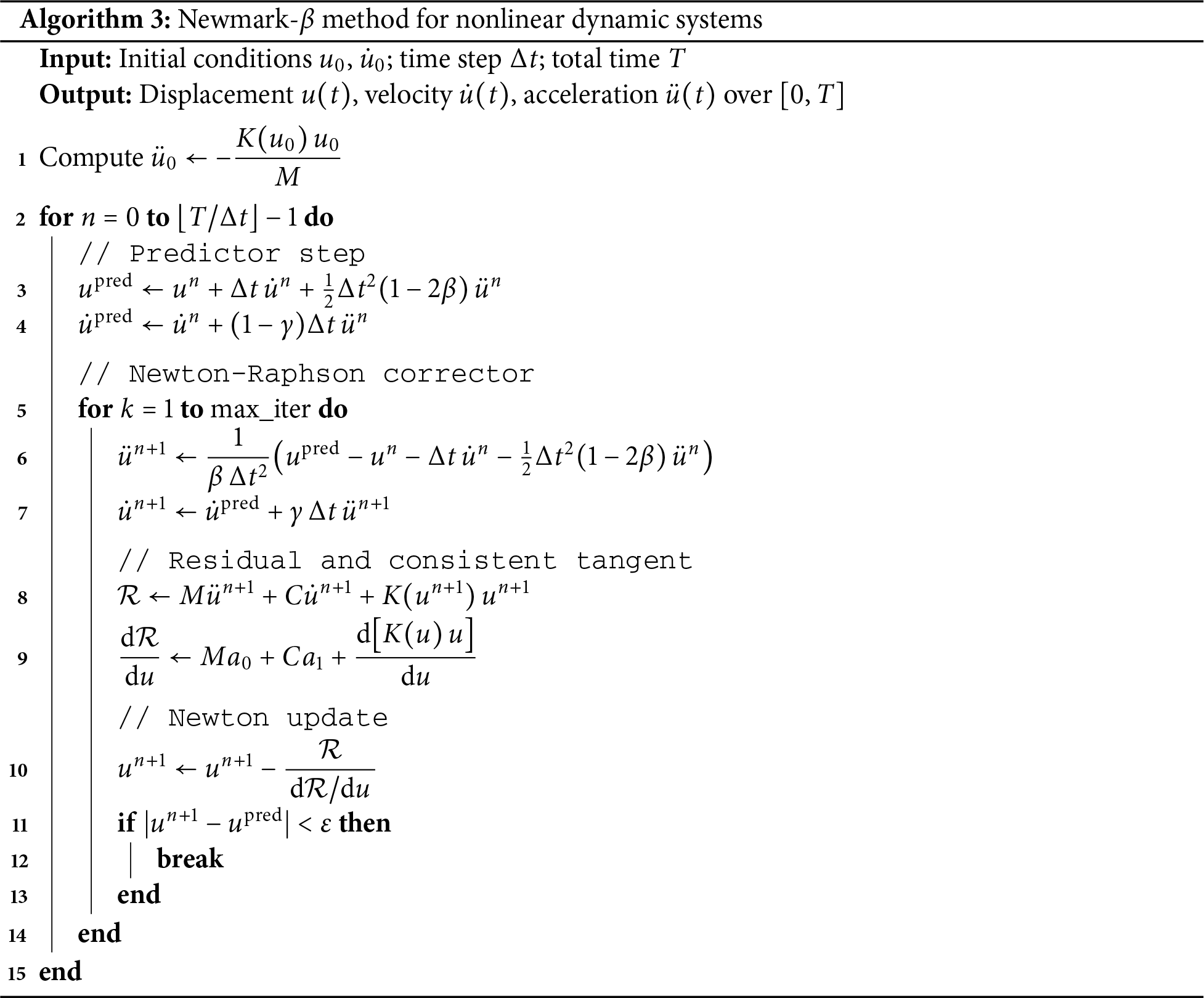
This setup provides highly accurate reference trajectories against which the PINN predictions are compared. The Newmark solution was also validated against the inbuilt Python solver solve_ivp, showing good agreement, as illustrated in Figs. 6 and 7 for the soft-stiffness case. It shows the evolution of displacement and velocity for an impact oscillator with time. The results are further consistent with those reported in the literature [2]. The good agreement of the figures with the literature and other numerical methods validates our approach.

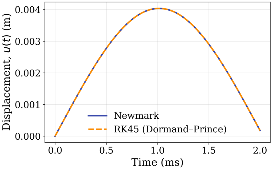
Figure 6: Comparison of displacement time histories from the Newmark and RK45 methods.

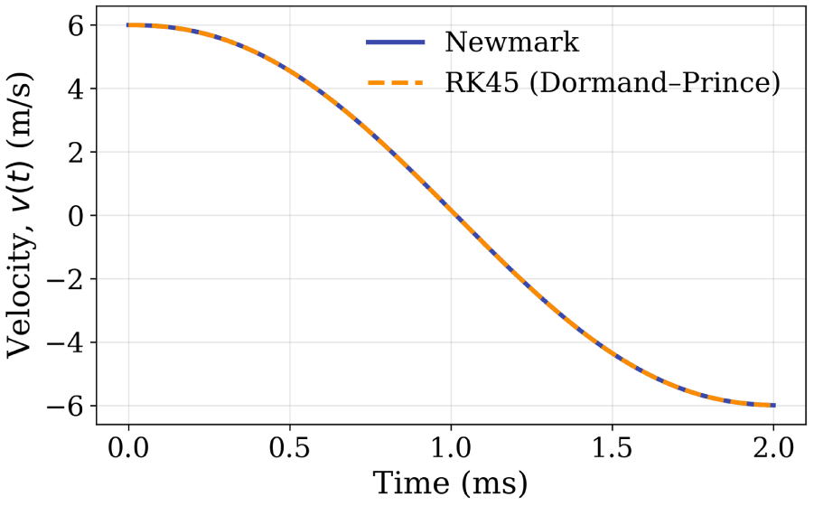
Figure 7: Velocity comparison between the Newmark and RK45 methods.

3  Results and Discussion

3.1 Forward Problem: Undamped Impact Oscillator

The nonlinear impact oscillator in the absence of damping (c = 0) is considered first. Each PINN is trained simultaneously using four initial velocities v0∈{2,3,4,6} m/s following the multi-condition approach described in Section 2.4. Results are presented for three stiffness regimes (soft, medium, and hard) and compared with the corresponding reference solutions obtained from Newmark-β time integration for each initial condition.

The soft stiffness case corresponds to the parameter set listed in Table 1, whose coefficients produce relatively smooth oscillatory responses. Figs. 8 and 9 show the displacement response and the corresponding relative L2 error, respectively, as predicted by the PINN and the Newmark method.

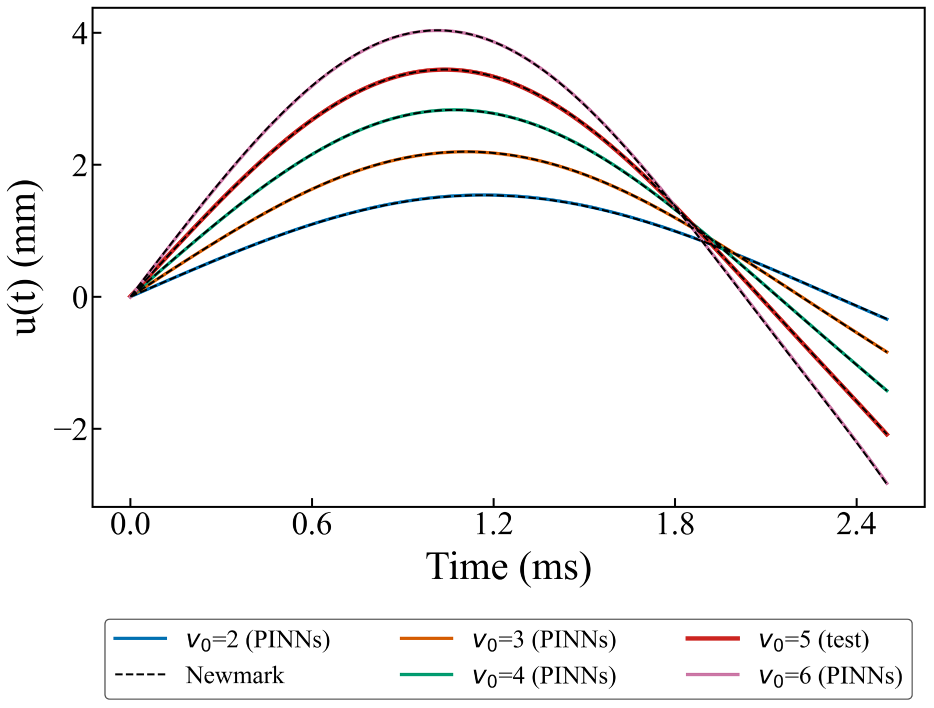
Figure 8: Comparison of displacement predictions for the soft-stiffness material without damping: PINN vs. Newmark method.

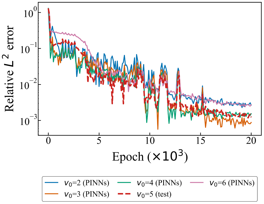
Figure 9: Relative L2 error of the predicted displacement for the soft-stiffness material without damping.

The two solutions exhibit close agreement over the full 2.4 ms simulation window, with the PINNs accurately reproducing both the amplitude envelope and the oscillation frequency for all three impact velocities. The relative L2 error settles at the order of 10−3 after approximately 20000 training epochs as shown in Fig. 6. Physically, the soft-stiffness regime is the most stable from a learning perspective. This is because the polynomial restoring force is dominated by its linear term (ω02), with the higher-order contributions activating only near peak displacement. This relatively smooth nonlinearity allows the network to capture the essential dynamics without encountering the sharp gradient changes that challenge standard PINNs. From an application standpoint, this regime corresponds to expanded polystyrene backing layers, where hail impacts produce distributed deformation rather than localized cracking. The PINN’s ability to resolve the full oscillation envelope at multiple impact velocities confirms that the multi-condition approach captures the energy-dependent contact mechanics governing this deformation mode. As the PINN model was trained for impact velocities of 2, 3, 4, and 6 m/s, its predictive performance was evaluated for both interpolation and extrapolation scenarios. For the interpolation case at 5 m/s, which lies within the training manifold, predictions were performed for all six impact configurations. The model achieved a computational speed-up of approximately 30 times compared with the Newmark solver for the soft undamped case, with an L2 error of 1.2217 × 10−3 as shown in Table 2. To assess extrapolation capability outside the training range, an additional prediction was performed for the soft undamped case only. In this instance, the model reported an error of approximately 5.7%, while retaining a speed-up of about 41 times relative to the Newmark solver as shown in Fig. 10.

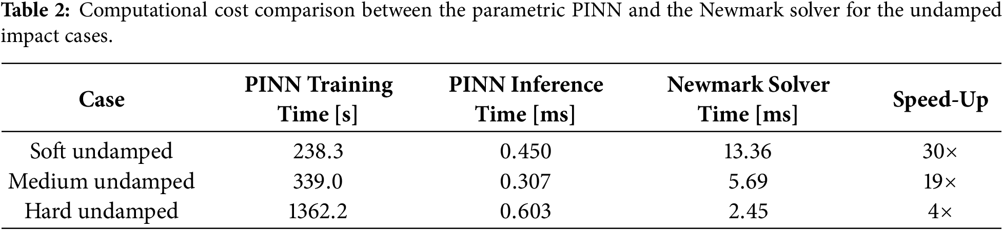
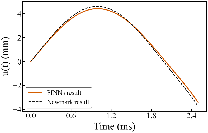
Figure 10: PINNs prediction for an extrapolation case for unseen velocity of 7 m/s.

For comparison, a vanilla neural network (NN) trained for an initial velocity of 6 m/s is shown in Fig. 11. The vanilla neural network reproduces the reference trajectory faithfully within its supervised training interval but diverges rapidly beyond it, as can be seen in Fig. 11. This comparison shows the specific contribution of the physics-informed loss, i.e., the governing equation residual acts as an inductive bias that constrains the network to the manifold of physically admissible trajectories. The physics loss also prevents the extrapolation failure that is characteristic of purely data-driven surrogates. For impact dynamics applications, where the goal is to predict the full contact oscillation sequence from a model trained on partial or heterogeneous data, this physics-constrained generalization is essential.

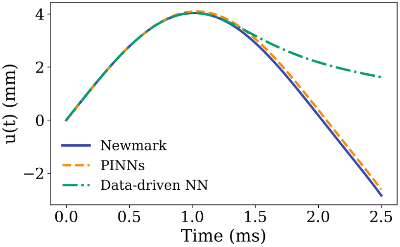
Figure 11: Comparison of PINN, NN, and Newmark solutions for the soft-stiffness material without damping, showing the predicted displacement.

Similarly, simulations were performed for the medium-stiffness case. Increasing the stiffness coefficients by roughly one to two orders of magnitude (Table 1) activates the higher-order polynomial terms more strongly. This results in a markedly sharper restoring force and a corresponding increase in oscillation frequency. Figs. 12 and 13 show that the PINN maintains accuracy at the 10−3 level, with amplitude and phase closely tracking the Newmark reference across all three initial velocities. The successful resolution of the medium regime is significant because the alveolar polycarbonate substrate it represents is among the most commonly used backing materials in commercial PV modules. The interplay between moderate compliance and the onset of significant nonlinear stiffening produces a response that is neither suitable to linearization nor so stiff as to be purely impulsive.

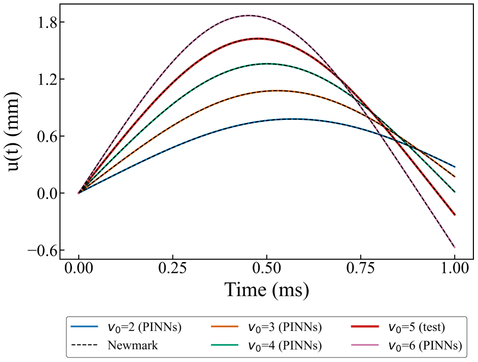
Figure 12: Comparison of predicted displacement for the medium-stiffness material without damping with the Newmark method.

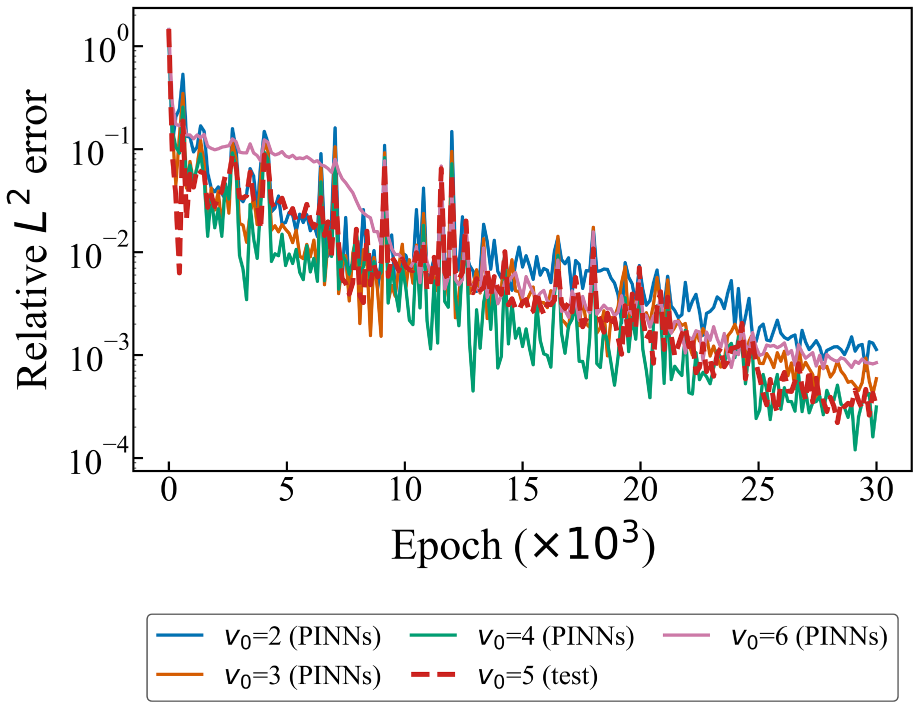
Figure 13: Relative L2 error of the predicted displacement for the medium-stiffness material without damping.

The numerical solution shows close agreement with the PINN predictions, with both amplitude and phase matching well throughout the plotted interval. The network successfully reproduces the higher oscillation frequency induced by the medium stiffness coefficients, accurately capturing the zero-crossings and peak displacements at the same time instants as the Newmark solution. For the medium and hard undamped cases, interpolation at an unseen velocity within the training range also produced errors of the order of 10−3. Table 2, confirms that the parametric PINN provides accurate forward predictions for new initial conditions while remaining approximately 19 and 4 times faster than the Newmark solver for medium and hard stiffness respectively.

In the hard-stiffness regime, the restoring force coefficients increase by a further one to two orders of magnitude, producing near-impulsive contact dynamics with sharp displacement peaks. Remarkably, the PINN achieves its lowest errors in this most challenging regime, with the relative L2 error reaching the order of 10−3 as seen in Figs. 14 and 15. This improvement can be attributed to the temporal compactness of the hard-impact pulse in which the displacement signal is effectively concentrated in a narrow time window. The response outside this window is nearly quiescent. The network therefore needs to resolve a sharp but localized feature rather than sustaining accuracy over many oscillation cycles. From the perspective of PV panel assessment, the hard regime, which represents a wooden-board substrate, corresponds to the highest-energy impacts that produce localized cracking and concentrated damage. The superior accuracy of the PINN in this regime is practically important because it is precisely the scenario where reliable contact force prediction is most critical for damage assessment.

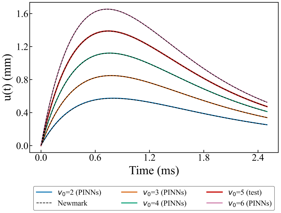
Figure 14: Comparison of displacement predictions for the hard-stiffness material without damping: PINN vs. Newmark method.

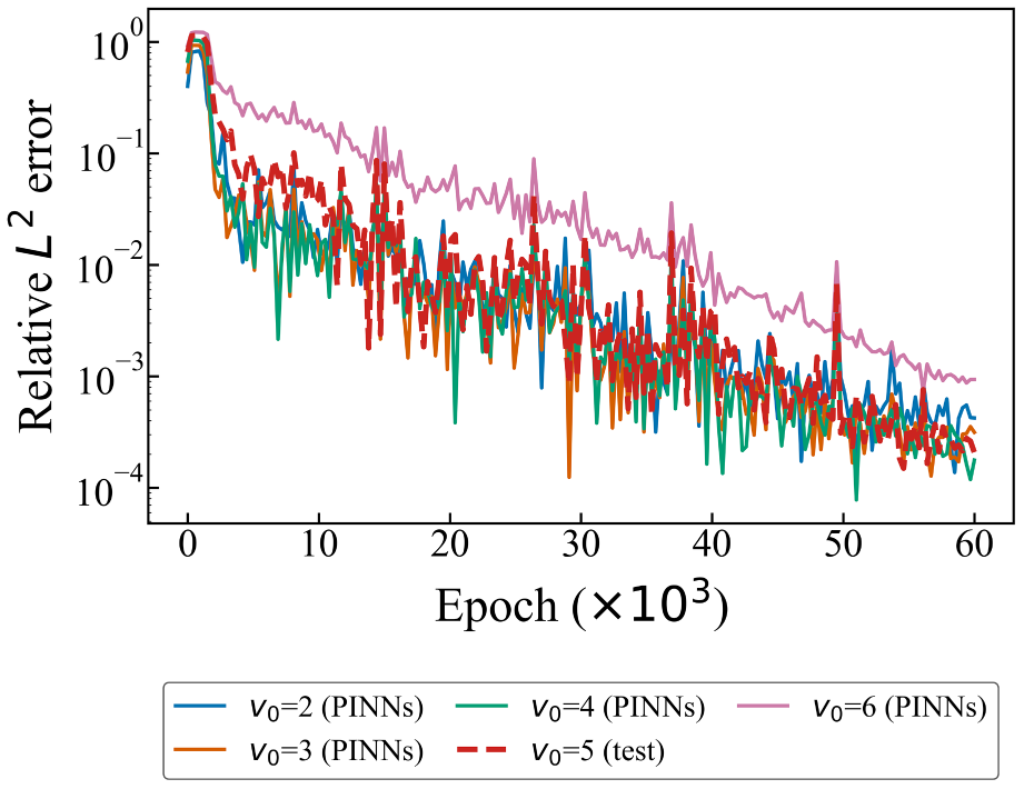
Figure 15: Relative L2 error of the predicted displacement for the hard-stiffness material without damping.

In contrast to the soft- and medium-stiffness cases, the error for the hard-stiffness material is on the order of 10−4.

3.2 Forward Problem: Damped Impact Oscillator

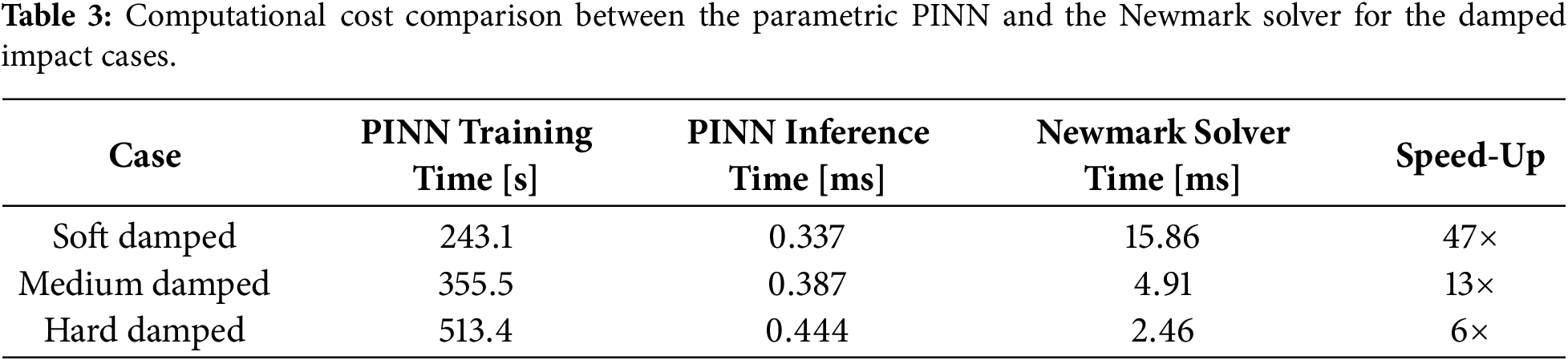
We now include viscous damping, which plays a dual role: physically, it dissipates energy and stabilizes the response; computationally, it regularizes the PINN optimization by suppressing long-horizon error accumulation. In real PV laminate systems, energy dissipation arises from viscoelastic material behavior in between the layers, and the effective damping level varies with temperature, loading rate, and material aging state. Modeling the damped response is therefore essential for capturing realistic post-impact oscillations. As in the undamped case, the PINN is trained simultaneously on three initial velocities v0∈{2,3,4,6} m/s. The simulations reported below use a damping coefficient per unit mass of c = 100 Ns/kgm.

The results for the soft-stiffness case with damping are presented in Figs. 16 and 17. The PINN solution shows excellent agreement with the Newmark reference over the entire simulation horizon. The introduction of damping alters the system response, and this change is accurately captured by the PINN. Moreover, damping reduces the sensitivity of the PINN to training inaccuracies by stabilizing the dynamics. While the minimum relative L2 error decreases, the overall error range remains comparable to that observed in the undamped cases, i.e., on the order of 10−1.

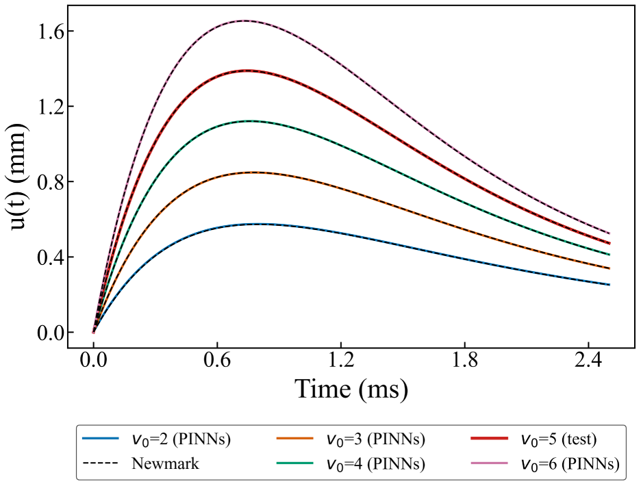
Figure 16: Comparison of displacement predictions for the soft-stiffness material with damping: PINN vs. Newmark method.

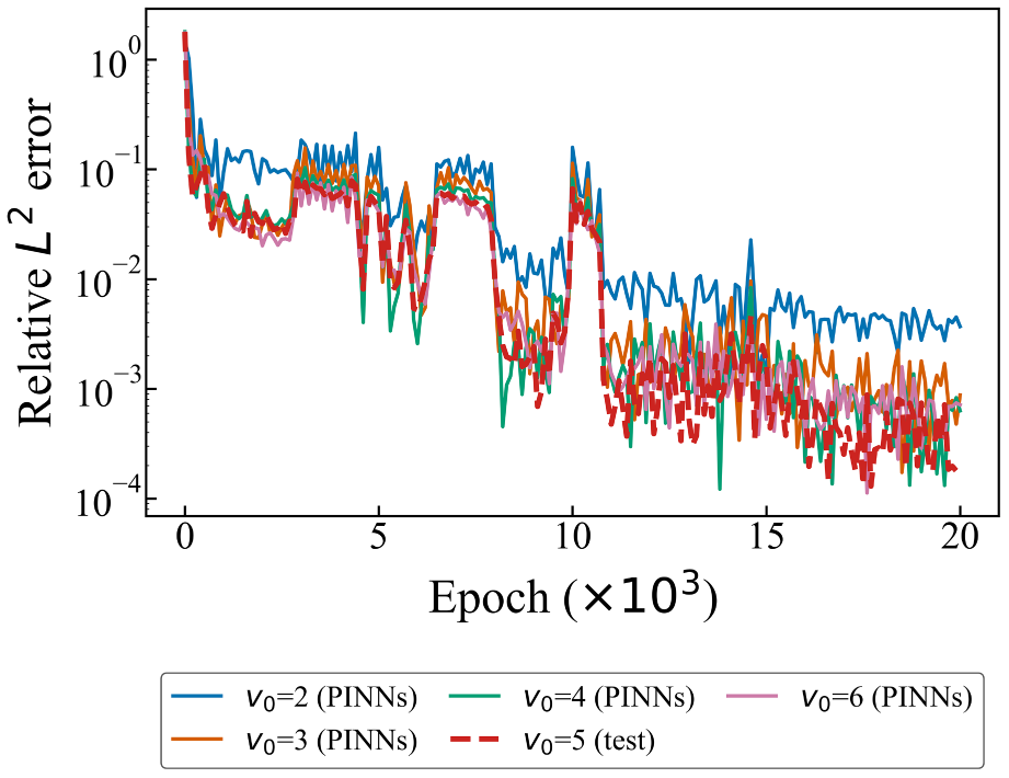
Figure 17: Relative L2 error of the predicted displacement for the soft-stiffness material with damping.

The medium-stiffness scenario with damping is presented in Figs. 18 and 19. The PINN again closely matches the Newmark solution, accurately capturing both the higher oscillation frequency and the dissipative decay. Notably, the number of training epochs required to reach the minimum error is reduced, as the relative error attains the order of 10−3 more quickly than in the undamped case. For the medium-stiffness scenario, damping provides stabilization both physically and numerically. Although the oscillator exhibits stiffer restoring forces and faster oscillations compared to the soft system, the PINN maintains high accuracy without requiring hybridization or modifications to the network architecture.

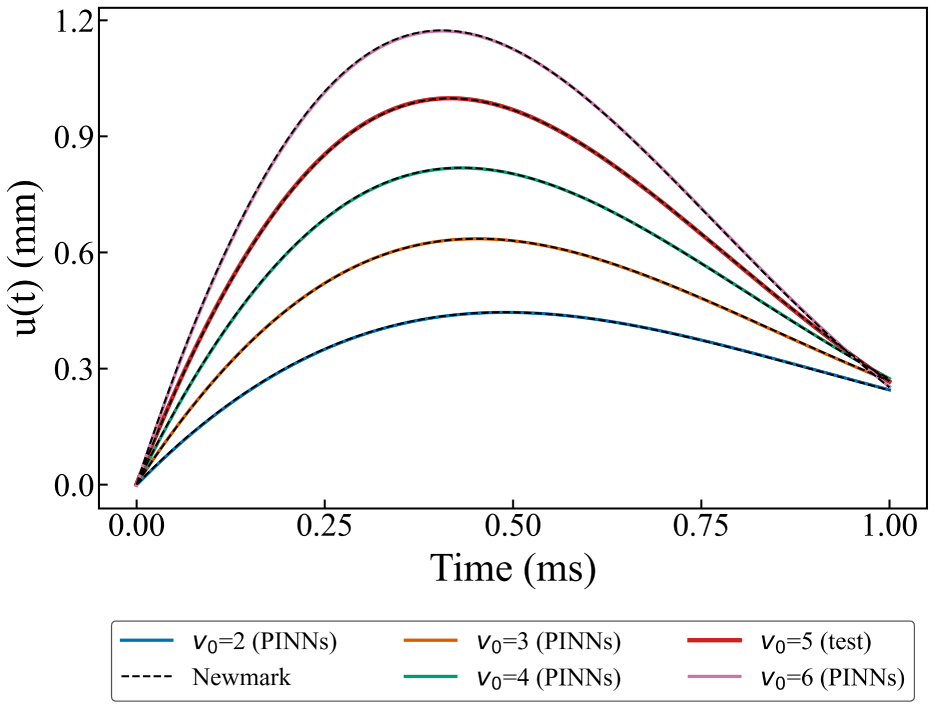
Figure 18: Comparison of displacement predictions for the medium-stiffness material with damping: PINN vs. Newmark method.

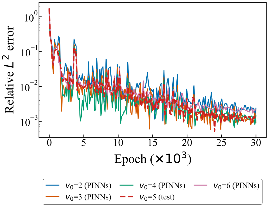
Figure 19: Relative L2 error of the predicted displacement for the medium-stiffness material with damping.

The hard-stiffness case with damping is presented in Figs. 20 and 21. Compared to the undamped counterpart, damping significantly delays the onset of deviations. The PINN accurately captures the initial oscillations and reproduces the decaying amplitude trend observed in the Newmark solution. Toward the end of the simulation horizon, some phase drift and slight underestimation of the displacement amplitude are observed; however, the errors remain smaller and accumulate more slowly than in the undamped case.

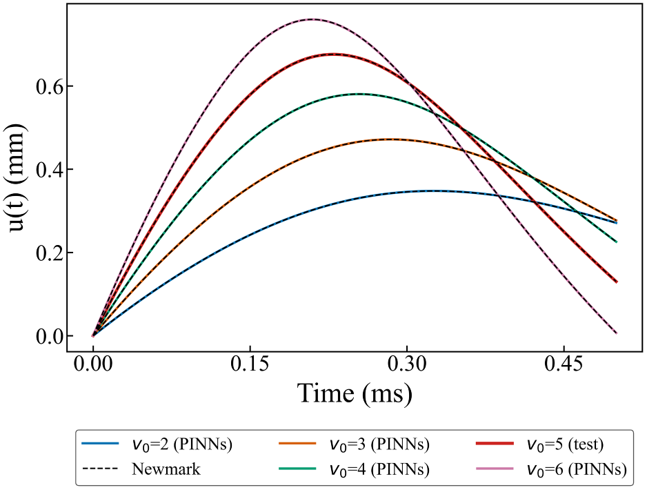
Figure 20: Comparison of displacement predictions for the hard-stiffness material with damping: PINN vs. Newmark method.

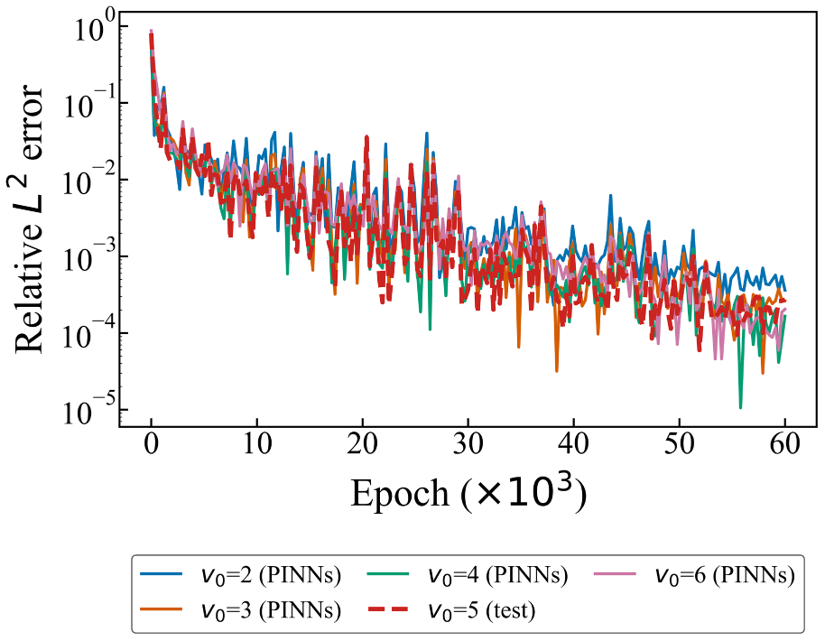
Figure 21: Relative L2 error of the predicted displacement for the hard-stiffness material with damping.

Similar to the undamped cases, interpolation tests were performed for the damped cases at the unseen velocity of 5 m/s within the training range. In all damped cases, the relative errors remained of the order of 10−3, confirming that the proposed parametric PINN maintains good predictive accuracy across different stiffness and damping regimes. The model also provided fast predictions for new initial conditions, with an average speed-up of approximately 47, 13 and 6 times for soft, medium and hard stiffness compared with the Newmark solver respectively, as shown in Table 3.

3.3 Benchmark Problem I: Damped Duffing Oscillator

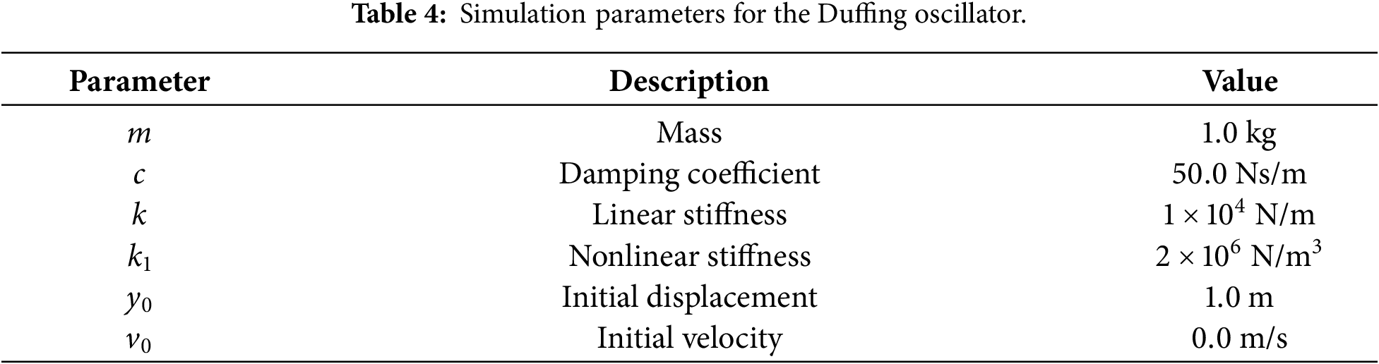
The Duffing oscillator is a canonical benchmark for nonlinear vibration analysis and is included here not as an additional application case but as an independent verification of the PINN framework on a well-characterized system with known analytical properties. It incorporates linear and cubic stiffness terms along with viscous damping, making it a representative test case for systems exhibiting hardening or softening nonlinearities. Parameter values are listed in Table 4, with initial conditions u(0)=1.0 m, and u˙(0)=0 m/s. The system exhibits strongly nonlinear, decaying oscillations under free vibration.

Before applying PINNs, the problem was solved using the Newmark-β method and validated against the high-order Radau solver in Python. Fig. 22 shows the displacement, while Fig. 23 presents the velocity vs. time for both methods. The two solutions are virtually indistinguishable, confirming that the Newmark scheme, combined with Newton-Raphson iteration for the nonlinear terms, provides a robust and accurate baseline. This step is crucial, as the performance of the PINN must be assessed against a reliable reference solution.

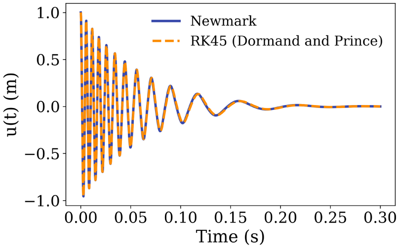
Figure 22: Comparison of displacement responses from the Newmark and RK45 methods for the Duffing oscillator.

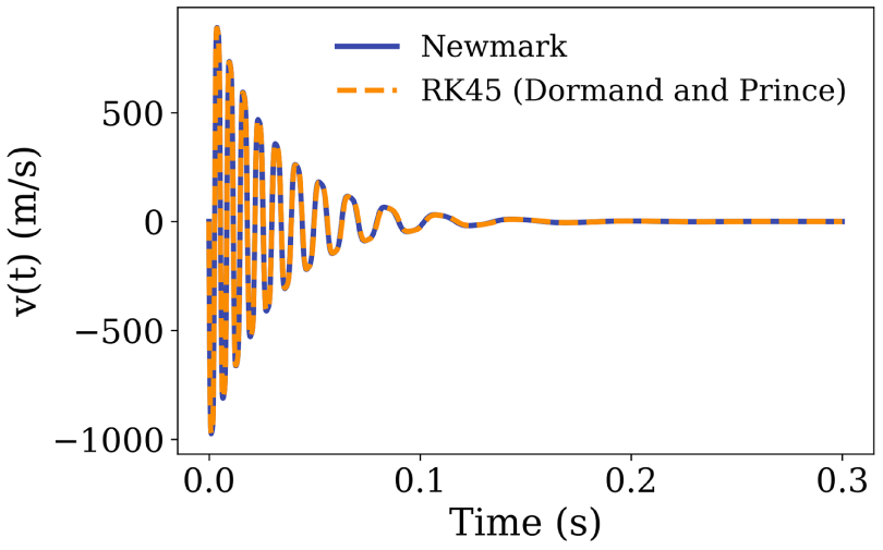
Figure 23: Comparison of velocity responses from the Newmark and RK45 methods for the Duffing oscillator.

Hybrid PINN Solution

A hybrid PINN was then applied to Eq. (9). Unlike the impact problem, where no data were used, the Duffing oscillator PINN incorporates both physics-informed residuals and partial supervised data over the first half of the time domain (t≤tmax/2).

The network architecture follows the setup described in Section 2.3, with two hidden layers of 64 neurons each and the tanh activation function. Inputs and outputs were non-dimensionalized using t∗=t/tmax and u∗=u/u0 to mitigate scaling issues.

The total loss function combines all the relevant loss terms and be written as in Eq. (34):

ℒtotal=ℒphys+ℒIC+λdataℒdata,(34)

where λdata controls the contribution of the supervised region.

The PINN was trained for 80,000 epochs using the Adam optimizer with a learning rate of 10−3. At each epoch, 200 collocation points were sampled across t∗∈[0,1], while reference data points for ℒdata were restricted to the first half of the time interval.

Figs. 24 and 25 show the PINN predictions compared with the reference numerical solution, along with the corresponding relative L2 error for the Duffing oscillator. Within the supervised interval (t≤0.10 s), the PINN closely matches the reference solution, accurately capturing both the amplitude decay and oscillation frequency. This demonstrates the benefit of incorporating partial supervised data. Quantitatively, the relative L2 error remains on the order of 10−2 throughout the time window, which is acceptable for nonlinear dynamics. The low residual values confirm that the governing physics are well satisfied at the collocation points. These results further highlight that including a supervised data loss term is essential for accurately reconstructing the nonlinear response; without it, model performance degrades significantly.

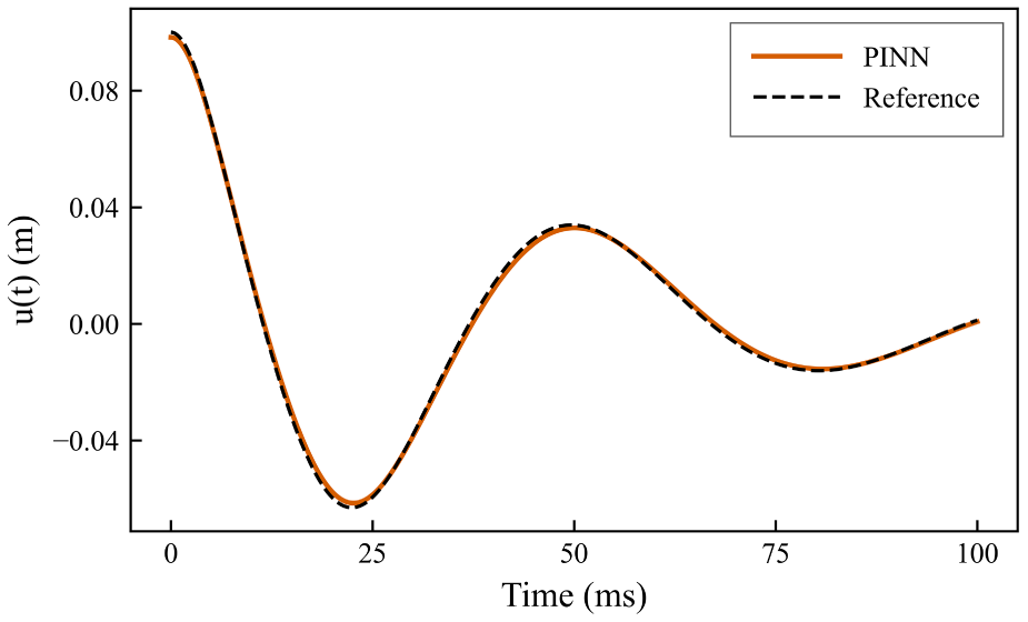
Figure 24: Performance of PINNs for the Duffing oscillator compared with the Newmark method.

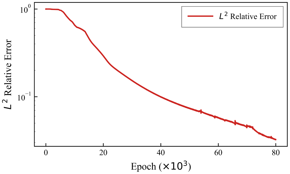
Figure 25: Relative L2 error of predicted displacement for the Duffing oscillator.

3.4 Benchmark Problem II: Nonlinear Belt–Mass System

The belt–mass system (Eq. (12)) represents a more complex nonlinear oscillator, incorporating viscous damping, quadratic damping, and cubic stiffness nonlinearities. This system provides a second independent verification case and is particularly relevant because the quadratic damping term c1u˙|u˙| introduces a nonlinearity in the dissipative forces, which is not present in any of the above cases. Such systems commonly arise in drive-belt and rotor dynamics, where both nonlinear damping and restoring forces significantly influence the response. Parameter values are summarized in Table 5, with initial displacement u(0)=0.01 m and velocity u˙(0)=0 m/s. The combination of linear and nonlinear damping along with cubic stiffness presents a challenging test for PINNs, due to the rapid decay of oscillations and strongly nonlinear dissipative effects. The system was first solved using the Newmark-β method and validated against the Radau solver in solve_ivp. Figs. 26 and 27 show close agreement between the two methods for both displacement and velocity over the 0.5 s simulation window. The solution exhibits rapid energy dissipation, with the amplitude decaying nearly to zero by the end of the interval. The strong nonlinear damping introduces asymmetry in the decay profile, which is accurately captured by both methods.

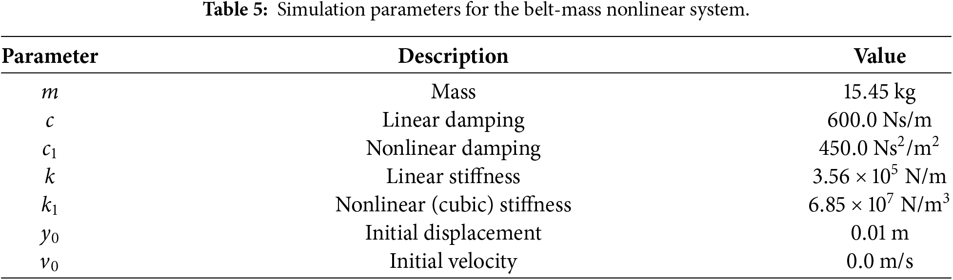
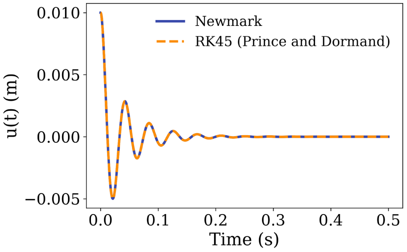
Figure 26: Displacement comparison between the Newmark and RK45 methods for the nonlinear Belt-Mass system.

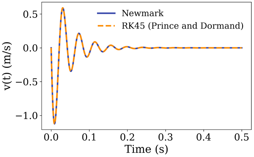
Figure 27: Velocity comparison between the Newmark and RK45 methods for the nonlinear Belt-Mass system.

Hybrid PINN Solution

A hybrid PINN was trained on the belt–mass system using the same architecture as in the previous setups, comprising two hidden layers of 64 neurons each with tanh activation functions. Inputs and outputs were nondimensionalized to enhance numerical stability. The loss function combined physics, initial condition, and supervised data terms, with the supervised contribution restricted to the first half of the simulation window (t≤0.25 s). The weighting factor for the data term, λdata, was initially set to 10.

Figs. 28 and 29 show the PINN predictions compared with the numerical solution and the corresponding relative L2 error, respectively. The PINN accurately reconstructs the nonlinear transient response within the supervised region, capturing both the amplitude and decay trend. In the unsupervised region, the network generalizes well but exhibits a slight underestimation of the amplitude decay. Convergence was relatively slow, requiring over 60,000 epochs to achieve acceptable accuracy, highlighting the challenge posed by stiff nonlinear damping for standard PINNs.

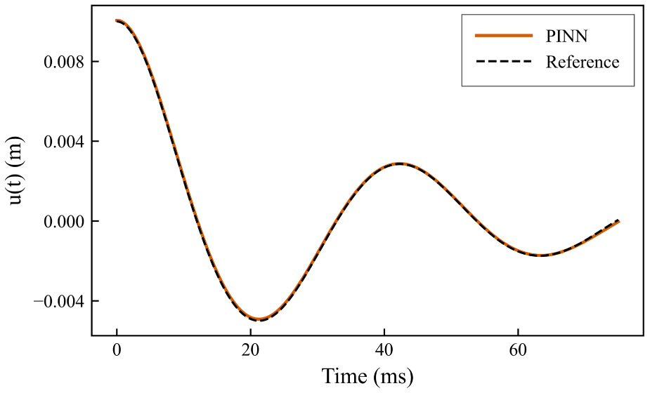
Figure 28: Performance of Hybrid PINNs for nonlinear Belt-Mass system compared with the Newmark method

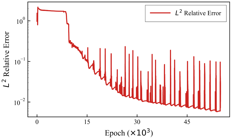
Figure 29: Relative L2 error of predicted displacement for the nonlinear Belt-Mass system.

3.5 Inverse Results

This section demonstrates the inverse capability of the proposed framework, i.e., recovering all governing physical coefficients from sparse displacement–velocity observations, without prior knowledge of the true parameter values. In the context of hail-impact assessment, this corresponds to the scenario of estimating the effective contact stiffness properties of a PV substrate in a simulation setting. The ability to perform such identification from sparse data is the principal engineering contribution of this work. The network is provided with Nd=300 uniformly sampled displacement–velocity observations (increased to 500 for overdamped cases) and no prior knowledge of the true parameters beyond a generic initial guess set at 50% of their true values.

3.5.1 Undamped Impact Cases

Table 6 summarizes the identified parameters for the three undamped stiffness regimes. All four coefficients (ω02,A,B,C) are recovered within 6% of their true values across all regimes, using only 300 sparse observations and an initial guess set at 50% of the ground truth. To place this accuracy in practical context, the coefficient differences between adjacent stiffness regimes in Table 6 span one to two orders of magnitude. So, a 6% identification error is therefore far smaller than the inter-regime separation, meaning the inverse PINN is able to classify which substrate type is present.

Fig. 30 shows the parameter convergence histories. During the initial warm-up phase, all parameters remain near their initial guesses. Once the alternating optimization with gradient-balanced physics loss commences, the parameters converge steadily toward their true values. The staircase-like pattern corresponds to the discrete LS updates at the start of each round, while the smooth plateaux during intermediate Adam epochs reflect the network’s refinement of the displacement field.

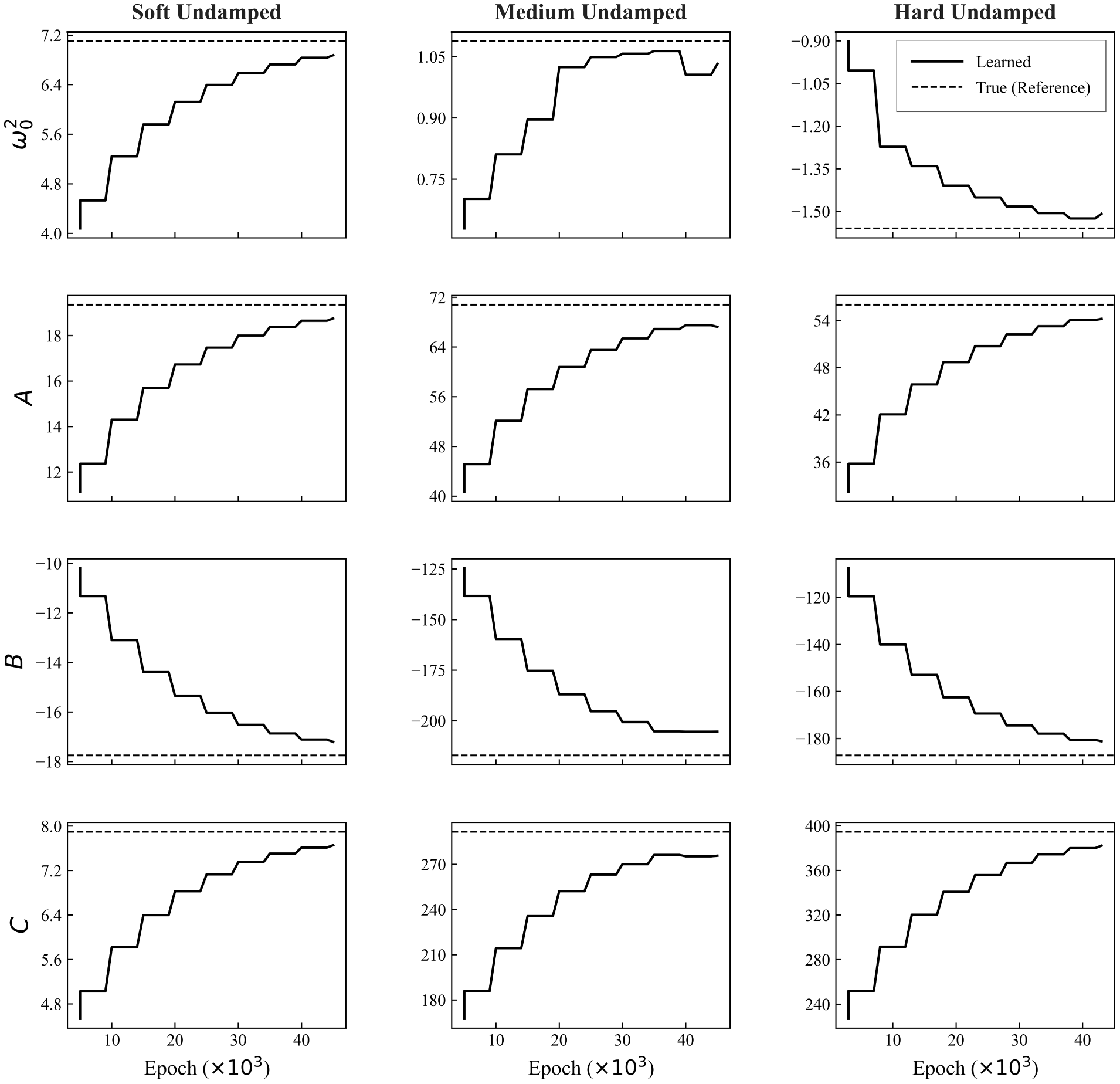
Figure 30: Parameter convergence histories for the three undamped impact cases (inverse PINN). Dashed lines indicate true values; final-epoch percentage errors are annotated.

3.5.2 Damped Impact Cases

For the damped cases, the inverse PINN also identifies the damping coefficient cs. Table 7 shows that the damping coefficient is recovered with 1% error in all three regimes while the nonlinear stiffness coefficients are recovered within 5% for all cases, with the medium damped configuration being the most challenging due to the interplay between moderate damping and intermediate stiffness. The consistently low error in the damping coefficient (≤1% across all regimes) is notable because damping governs the energy dissipation rate and directly influences the post-impact oscillation that would be recorded by a sensor. Accurate recovery of both stiffness and damping parameters from the same sparse dataset demonstrates that the inverse framework can simultaneously characterize the elastic contact response and the viscoelastic dissipation. These two mechanically distinct properties that are both essential for comprehensive damage assessment of a PV panel.

Fig. 31 reveals distinct convergence behaviours across damping regimes. The hard damped case (ζ≈0.53, underdamped) converges smoothly and rapidly. The soft damped case (ζ≈1.25, overdamped) requires a longer warm-up (Nw=25,000) and intra-round LS updates every 200 epochs to overcome the near-collinearity of the design matrix columns induced by the monotone pulse trajectory. The medium damped case converges steadily but requires the most rounds (Nr=12) to reach its final accuracy.

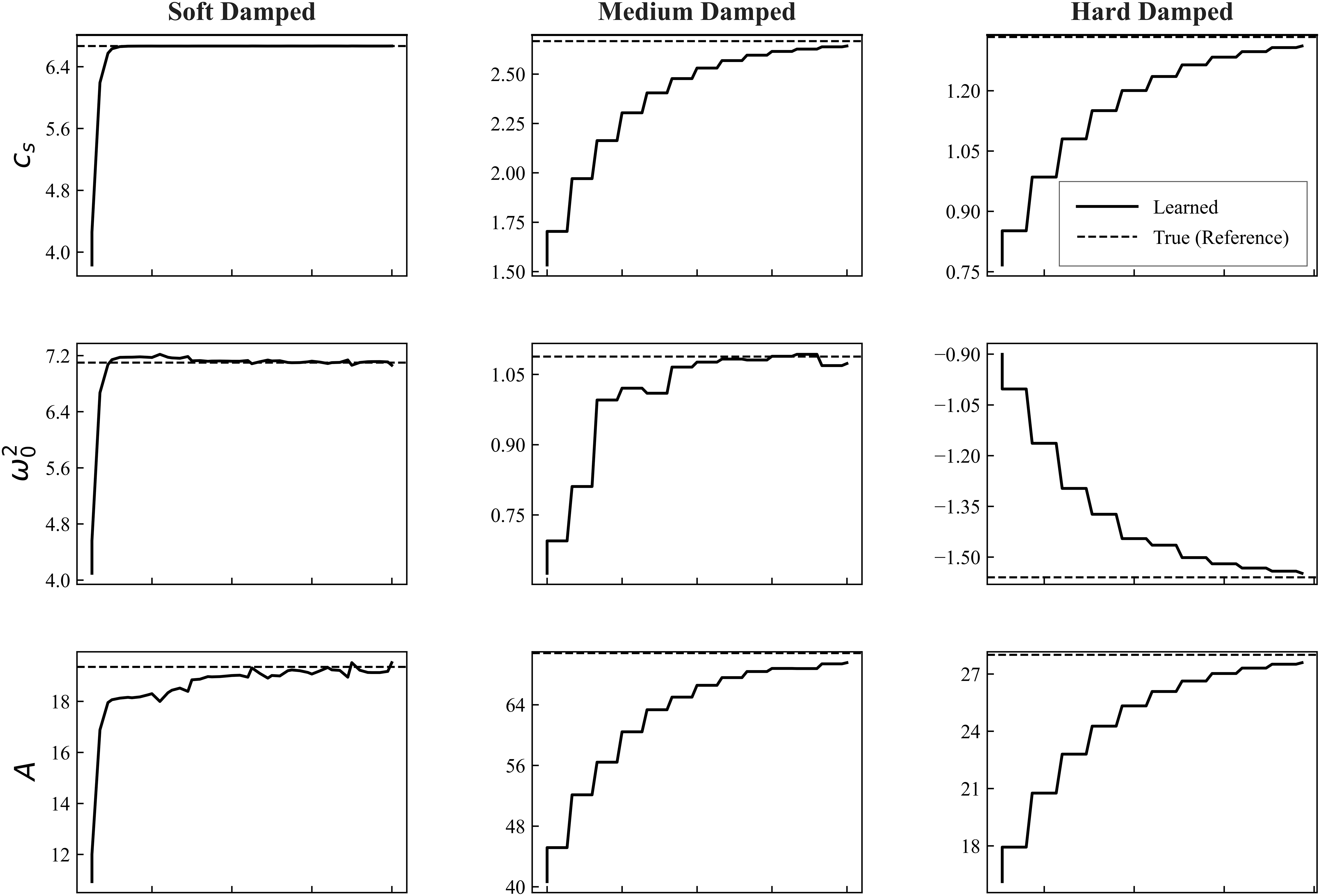
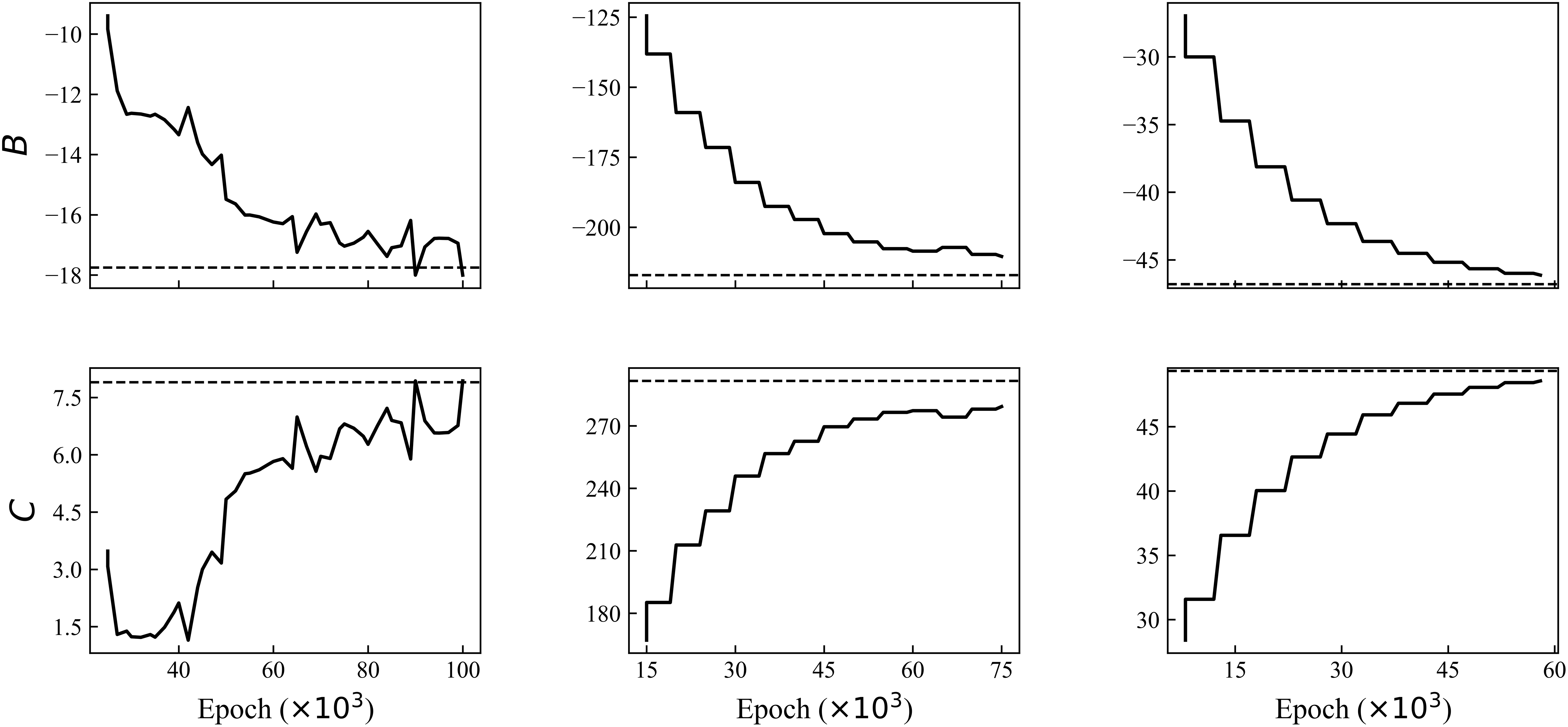
Figure 31: Parameter convergence for the three damped impact cases (inverse PINN). The damping coefficient cs (top row) is recovered with high precision in all regimes.

3.5.3 Benchmark Inverse Problems

Table 8 reports the results for the Duffing oscillator and the belt-mass system. Both the systems are treated with the full inverse PINN framework (data + IC + physics), with the physics loss evaluated as a strong-form collocation residual at 500 uniformly spaced interior points.

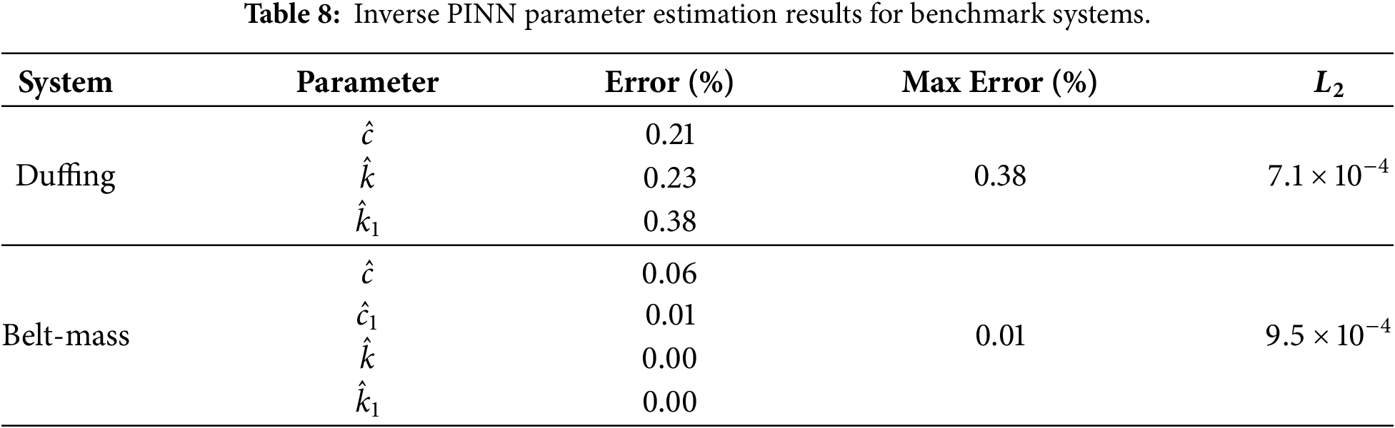
All benchmark parameters are recovered with errors below 0.4%, as shown in Fig. 32. It confirms that the current strategy is not specific to the polynomial restoring force structure of the impact oscillator. The belt–mass system is especially instructive because its quadratic damping term c1u˙|u˙| is structurally different from anything in the impact ODE, yet the inverse methodology recovers the coefficient with negligible error (0.01%). This portability across qualitatively different nonlinearities strengthens confidence in the framework’s applicability to other impact and vibration problems beyond the specific systems studied here.

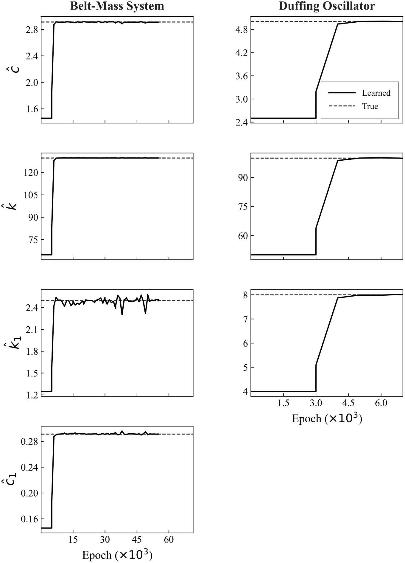
Figure 32: Parameter convergence for the benchmark inverse cases. Left: belt-mass system (4 parameters including quadratic damping c^1). Right: Duffing oscillator (3 parameters; c^1 row absent).

3.5.4 Inverse Parameters Estimations with Noise

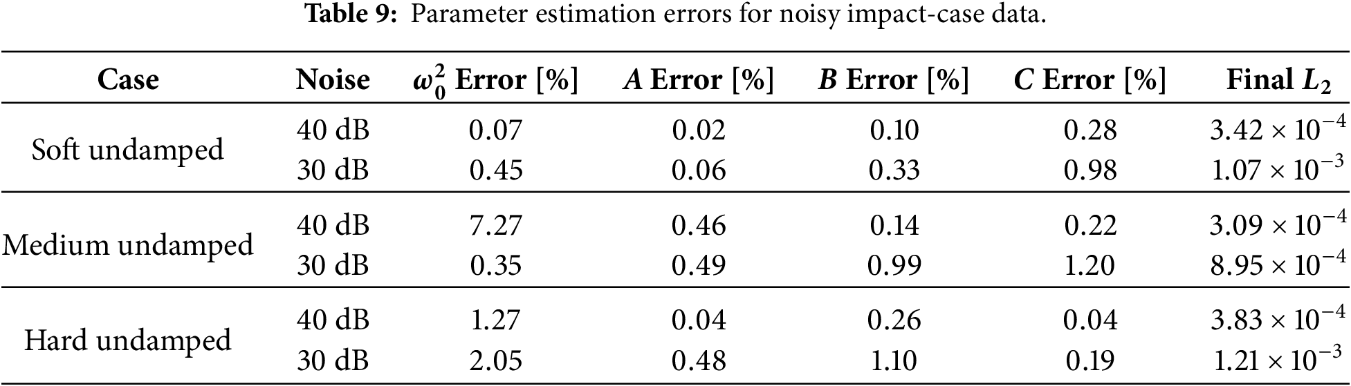
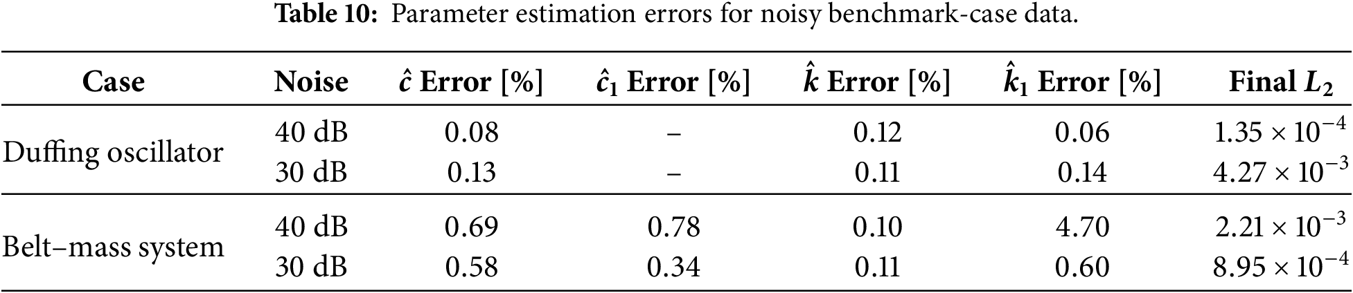
The inverse problem was extended by adding gaussian noise to the data obtained from the Newmark solver, to test the scenario of real data potentially acquired by sensors. The results are listed in Tables 9 and 10 and show that our methodology remains reasonably robust to moderate noise.

3.5.5 Quantitative Uncertainty Quantification

To assess the influence of the equivalent SDOF assumption, a bootstrap-based uncertainty analysis was performed for the soft undamped case using 15 repeated identification runs, as shown in Fig. 33. The estimated distributions of ω02, A, B, and C show that the corresponding true values remain within the 95% confidence intervals. The uncertainty remains relatively limited for ω02, A, and B, whereas the largest variation is observed for the higher-order coefficient C, with an approximate deviation of up to 5%. These results indicate that the SDOF approximation provides stable effective parameter estimates for the present case, although higher-order nonlinear coefficients may be more sensitive when the lumped-model assumption is violated.

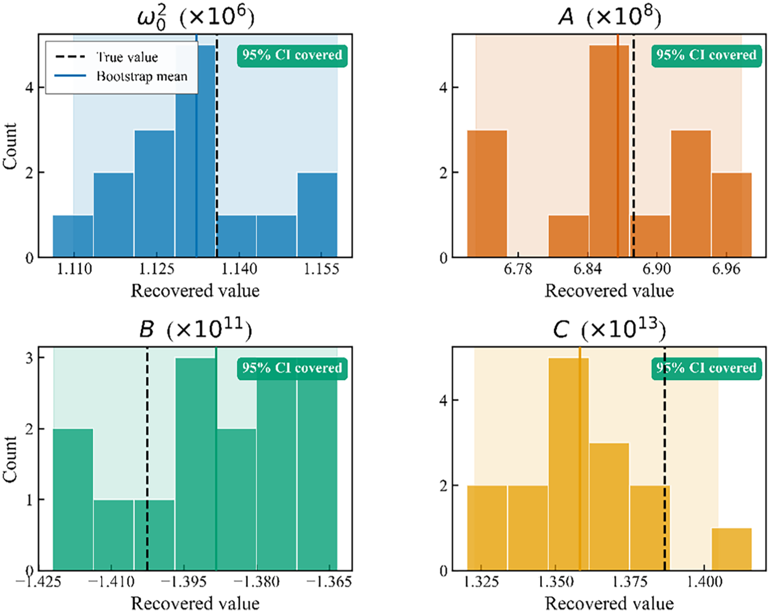
Figure 33: Bootstrap-based uncertainty analysis for the inverse parameters estimation.

3.5.6 Role of Gradient Balancing

The gradient-balanced physics weighting (Eq. (31)) is the key ingredient that enables the inverse PINN to function reliably. Without it, the physics loss produces large, misdirected gradients that corrupt the data-learned displacement field. The exponential ramp provides an additional layer of protection during early training, ensuring that the physics contribution remains negligible until the LS has had several rounds to refine the parameters toward physically meaningful values.

To examine the influence of the gradient-balancing ratio (α) on the inverse-identification accuracy, an ablation study was performed for the soft undamped case. Four representative values, α = 0.01, 0.1, 0.5, and 1.0, were tested. The results shows that the lowest maximum error, equal to 3.19%, was obtained for α = 0.1 as shown in Table 11. Therefore, this value was adopted in the inverse-identification experiments other than for soft damped case.

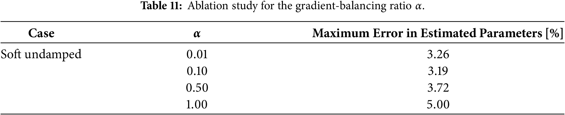
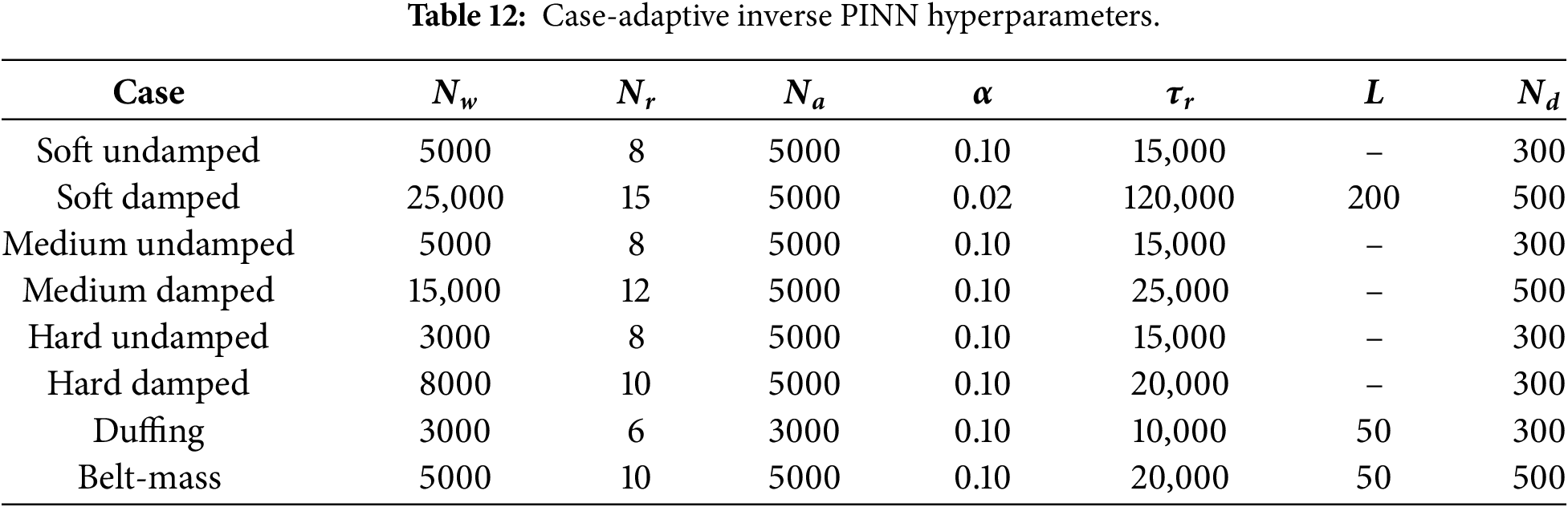
Table 12 lists the case-adaptive hyperparameters. The gradient-balance ratio α ranges from 0.02 (soft damped, where the overdamped trajectory makes the physics loss particularly aggressive) to 0.1 (standard cases). The ramp time constant τr is set proportionally to the total Phase 2 epoch count. These settings were determined through a small number of preliminary runs and remained fixed across all subsequent experiments.

4  Conclusion and Future Perspectives

This work has developed and validated a Physics-Informed Neural Network frame work for hail-induced impact dynamics, addressing both forward simulation and inverse parameter estimation across soft, medium, and hard stiffness regimes with and without viscous damping. For the forward problem, the multi-condition PINN reproduced the Newmark-β reference trajectories with relative L2 errors of order 10−3 for the soft and medium stiffness regimes and 10−4 for the hard regime, across all three impact velocities and both undamped and damped configurations. The accuracy gain in the hardest case reflects the temporal compactness of near-impulsive contact in which the network resolves a sharp but localized feature rather than sustaining precision over many oscillation cycles. By introduction of viscous damping, the training was stabilized and the target error level required approximately half the number of epochs of the corresponding undamped cases. The predictive performance of the PINN was evaluated across both interpolation and extrapolation scenarios. For interpolation at an initial velocity of 5 m/s, the model achieved computational speed-ups of approximately 30×, 19×, and 4× for soft, medium, and hard undamped conditions, respectively. Furthermore, in an extrapolation scenario at 7 m/s, the model demonstrated a 40× speed-up for the soft undamped case.

For the inverse problem, a two-phase algorithm was adopted which decoupled the learning tasks that destabilize the joint optimization. The physical coefficient updates was carried out by least squares method and its stability was ensured by a physics loss contribution. Across the six impact configurations, all stiffness coefficients, i.e., ω02,A,B,C were recovered within 6% of ground truth from 300 sparse displacement–velocity samples. On the two independent benchmarks, the Duffing oscillator and the belt–mass system with linear and quadratic dissipation the parameter errors dropped below 0.4%, demonstrating that the approach is not specific to the polynomial structure of the impact ODE but can be extended to nonlinearities located in the dissipative terms as well.

From the standpoint of photovoltaic module assessment, the practical implication is direct. Because the coefficient differences between soft, medium and hard substrates span one to two orders of magnitude, so a 6% identification error discriminates substrate type unambiguously. the inverse methodology was evaluated using data corrupted by Gaussian noise, demonstrating robust noise insensitivity. The current study can be extended in various directions, such as deploying and testing the inverse model on experimental data to ensures its practicality for real world scenarios. Finally, a meta learning strategy could be adopted in which a neural network would learn the context of the training, i.e., mapping the inputs to the outputs and would ensure that all the possibilities around this problem could be covered.

Acknowledgement: None.

Funding Statement: The authors received no specific funding for this study.

Author Contributions: The authors confirm contribution to the paper as follows: Conceptualization, Hassaan Idrees, Pattabhi Ramaiah Budarapu, Marco Paggi; methodology, Hassaan Idrees, Pattabhi Ramaiah Budarapu, Marco Paggi; validation, Hassaan Idrees, Pattabhi Ramaiah Budarapui; formal analysis, Hassaan Idrees, Pattabhi Ramaiah Budarapu, Marco Paggi; resources, Pattabhi Ramaiah Budarapu, Marco Paggi; data curation, Hassaan Idrees, Pattabhi Ramaiah Budarapu; writing—original draft preparation, Hassaan Idrees; writing—review and editing, Pattabhi Ramaiah Budarapu, Marco Paggi; visualization, Hassaan Idrees; project administration, Pattabhi Ramaiah Budarapu, Marco Paggi. All authors reviewed and approved the final version of the manuscript.

Availability of Data and Materials: All data generated or analysed during this study are included in this published article.

Ethics Approval: Not applicable.

Conflicts of Interest: Given his role as Editorial Board Member of this journal, Marco Paggi had no involvement in the peer review of this article and had no access to information regarding its peer review. Full responsibility for the editorial process for this article was delegated to another journal editor. The authors declare no other conflicts of interest.

References

1. Jäger-Waldau A. Snapshot of photovoltaics—May 2023. EPJ Photovolt. 2023;14:23. [Google Scholar]

2. Corrado M, Infuso A, Paggi M. Simulated hail impacts on flexible photovoltaic laminates: testing and modelling. Meccanica. 2017;52(6):1425–39. doi:10.1007/s11012-016-0483-2. [Google Scholar] [CrossRef]

3. Newmark NM. A method of computation for structural dynamics. J Eng Mech Div. 1959;85(3):67–94. doi:10.1061/jmcea3.0000098. [Google Scholar] [CrossRef]

4. Raissi M, Perdikaris P, Karniadakis GE. Physics-informed neural networks: a deep learning framework for solving forward and inverse problems involving nonlinear partial differential equations. J Comput Phys. 2019;378:686–707. [Google Scholar]

5. Cuomo S, Di Cola V, Schiano GF, Rozza G, Raissi M, Piccialli F. Scientific machine learning through physics-informed neural networks: where we are and what’s next. J Sci Comput. 2022;92(3):88. [Google Scholar]

6. Karniadakis GE, Kevrekidis IG, Lu L, Perdikaris P, Wang S, Yang L. Physics-informed machine learning. Nat Rev Phys. 2021;3(6):422–40. doi:10.1038/s42254-021-00314-5. [Google Scholar] [CrossRef]

7. Chen Z, Liu Y, Sun H. Physics-informed learning of governing equations from scarce data. Nat Commun. 2021;12(1):6136. doi:10.1038/s41467-021-26434-1. [Google Scholar] [CrossRef]

8. Pang G, Lu L, Karniadakis GE. fPINNs: fractional physics-informed neural networks. SIAM J Sci Comput. 2019;41(4):A2603–26. doi:10.1137/18m1229845. [Google Scholar] [CrossRef]

9. Raissi M, Perdikaris P, Ahmadi N, Karniadakis GE. Physics-informed neural networks and extensions. arXiv:2408.16806. 2024. [Google Scholar]

10. Luo K, Zhao J, Wang Y, Li J, Wen J, Liang J, et al. Physics-informed neural networks for PDE problems: a comprehensive review. Artif Intell Rev. 2025;58(10):1–43. doi:10.1007/s10462-025-11322-7. [Google Scholar] [CrossRef]

11. Sophiya AA, Nair AK, Maleki S, Krishnababu SK. A comprehensive analysis of PINNs: variants, applications, and challenges. arXiv:2505.22761. 2025. [Google Scholar]

12. Barbulescu R, Ciuprina G, Duca A, Machado P, Silveira LM. Physics-informed neural networks for a highly nonlinear dynamic system. J Math Ind. 2025;15(1):7. doi:10.1186/s13362-025-00172-1. [Google Scholar] [CrossRef]

13. Goswami S, Bora A, Yu Y, Karniadakis GE. Physics-informed deep neural operator networks. In: Machine learning in modeling and simulation: methods and applications. Cham, Switzerland: Springer; 2023. p. 219–54. [Google Scholar]

14. Mandl L, Goswami S, Lambers L, Ricken T. Separable physics-informed DeepONet: breaking the curse of dimensionality in physics-informed machine learning. Comput Methods Appl Mech Eng. 2025;434:117586. [Google Scholar]

15. Sahin T, von Danwitz M, Popp A. Solving forward and inverse problems of contact mechanics using physics-informed neural networks. Adv Model Simul Eng Sci. 2024;11(1):11. doi:10.1186/s40323-024-00265-3. [Google Scholar] [CrossRef]

16. Haywood AM, Arcieri G, Kamariotis A, Chatzi E. Response estimation and system identification of dynamical systems via physics-informed neural networks. Adv Model Simul Eng Sci. 2025;12(1):8. doi:10.1186/s40323-025-00291-9. [Google Scholar] [CrossRef]

17. Cardoso-Bihlo E, Bihlo A. Exactly conservative physics-informed neural networks and deep operator networks for dynamical systems. Neural Netw. 2025;181(6):106826. doi:10.1016/j.neunet.2024.106826. [Google Scholar] [CrossRef]

18. Stiasny J, Zhang B, Chatzivasileiadis S. PINNSim: a simulator for power system dynamics based on physics-informed neural networks. Elect Power Syst Res. 2024;235:110796. [Google Scholar]

19. Zhu Y, Yan Y, Zhang Y, Zhou Y, Zhao Q, Liu T, et al. Application of physics-informed neural network (PINN) in the experimental study of vortex-induced vibration with tunable stiffness. In: Proceedings of the 33rd International Ocean and Polar Engineering Conference; 2023 Jun 19–23; Ottawa, Canada. p. ISOPE-I. [Google Scholar]

20. Shaikh SA, Cherukuri H, Khan T. Recovering the forcing function in systems with one degree of freedom using ANN and physics information. Algorithms. 2023;16(5):250. doi:10.3390/a16050250. [Google Scholar] [CrossRef]

21. Rahaman N, Baratin A, Arpit D, Draxler F, Lin M, Hamprecht F, et al. On the spectral bias of neural networks. In: Proceedings of the 36th International Conference on Machine Learning; 2019 Jun 9–15; Long Beach, CA, USA. p. 5301–10. [Google Scholar]

22. Wang S, Yu X, Perdikaris P. When and why PINNs fail to train: a neural tangent kernel perspective. J Comput Phys. 2022;449:110768. [Google Scholar]

23. Krishnapriyan A, Gholami A, Zhe S, Kirby R, Mahoney MW. Characterizing possible failure modes in physics-informed neural networks. Adv Neural Inf Process Syst. 2021;34:26548–60. [Google Scholar]

24. Cao Y, Fang Z, Wu Y, Zhou DX, Gu Q. Towards understanding the spectral bias of deep learning. arXiv:1912.01198. 2019. [Google Scholar]

25. Waheed UB. Kronecker neural networks overcome spectral bias for PINN-based wavefield computation. IEEE GeosciRemote Sens Lett. 2022;19:1–5. doi:10.1109/lgrs.2022.3209901. [Google Scholar] [CrossRef]

26. Ding W, He Q, Tong H, Wang Q, Wang P. Solving coupled differential equation groups using PINO-CDE. Mech Syst Signal Process. 2024;208(4):111014. doi:10.1016/j.ymssp.2023.111014. [Google Scholar] [CrossRef]

27. Zhang R, Liu Y, Sun H. Physics-guided convolutional neural network (PhyCNN) for data-driven seismic response modeling. Eng Struct. 2020;215(5):110704. doi:10.1016/j.engstruct.2020.110704. [Google Scholar] [CrossRef]

28. Lai Z, Mylonas C, Nagarajaiah S, Chatzi E. Structural identification with physics-informed neural ordinary differential equations. J Sound Vib. 2021;508(2):116196. doi:10.1016/j.jsv.2021.116196. [Google Scholar] [CrossRef]

29. Haghighat E, Raissi M, Moure A, Gomez H, Juanes R. A physics-informed deep learning framework for inversion and surrogate modeling in solid mechanics. Comput Methods Appl Mech Eng. 2021;379(7553):113741. doi:10.1016/j.cma.2021.113741. [Google Scholar] [CrossRef]

30. Linka K, Schäfer A, Meng X, Zou Z, Karniadakis GE, Kuhl E. Bayesian physics informed neural networks for real-world nonlinear dynamical systems. Comput Methods Appl Mech Eng. 2022;402(9):115346. doi:10.1016/j.cma.2022.115346. [Google Scholar] [CrossRef]

31. Zhai W, Tao D, Bao Y. Parameter estimation and modeling of nonlinear dynamical systems based on Runge–Kutta physics-informed neural network. Nonlinear Dyn. 2023;111(22):21117–30. doi:10.1007/s11071-023-08933-6. [Google Scholar] [CrossRef]

32. Raj NNB, Banerjee S. FIM-guided PINNs for real-time parameter identification in digital twins of nonlinear vibratory systems. Knowl Based Syst. 2026;335:115198. [Google Scholar]

33. Chuang PY, Barba LA. Experience report of physics-informed neural networks in fluid simulations: pitfalls and frustration. arXiv:2205.14249. 2022. [Google Scholar]

34. Hao Z, Yao J, Su C, Su H, Wang Z, Lu F, et al. PINNacle: a comprehensive benchmark of physics-informed neural networks for solving PDEs. arXiv:2306.08827. 2023. [Google Scholar]

35. Grossmann TG, Komorowska UJ, Latz J, Schönlieb CB. Can physics-informed neural networks beat the finite element method? arXiv:2302.04107. 2023. [Google Scholar]

36. Cho W, Jo M, Lim H, Lee K, Lee D, Hong S, et al. Parameterized physics-informed neural networks for parameterized PDEs. arXiv:2408.09446. 2024. [Google Scholar]

37. Li J, Chen JB. Stochastic dynamics of structures. Singapore: John Wiley & Sons; 2009. [Google Scholar]

38. Lyu MZ, Chen JB. A unified formalism of the GE-GDEE for generic continuous responses and first-passage reliability analysis of multi-dimensional nonlinear systems subjected to non-white-noise excitations. Struct Saf. 2022;98(4):102233. doi:10.1016/j.strusafe.2022.102233. [Google Scholar] [CrossRef]

39. Ma F, Zhang H, Bockstedte A, Foliente GC, Paevere P. Parameter analysis of the differential model of hysteresis. J Appl Mech. 2004;71(3):342–9. doi:10.1115/1.1668082. [Google Scholar] [CrossRef]

40. Ge X, Luo Z, Ma Y, Liu H, Zhu Y. A novel data-driven model based parameter estimation of nonlinear systems. J Sound Vib. 2019;453(3):188–200. doi:10.1016/j.jsv.2019.04.024. [Google Scholar] [CrossRef]

41. Wang S, Teng Y, Perdikaris P. Understanding and mitigating gradient flow pathologies in physics-informed neural networks. SIAM J Sci Comput. 2021;43(5):A3055–81. doi:10.1137/20m1318043. [Google Scholar] [CrossRef]