STP-BTDM: Semi-Tensor Product-Based Block Term Decomposition of Multilinear Pooling Method for Multi-Modal Information Fusion in Sentiment Analysis

1  Introduction

Multi-modal information fusion refers to the integration of data from multiple modalities to facilitate more accurate and comprehensive predictive outcomes [1]. Compared to using only single-modality information, multimodal fusion can effectively integrate complementary data from different modalities, thus improving the performance of classification or prediction tasks. Recent studies have demonstrated the benefits of multi-modal fusion across a variety of fields, such as multi-modal speech recognition [2,3], sentiment analysis [4–6], and medical diagnosis. These studies highlight that integrating information from different modalities significantly contributes to increased accuracy and robustness. However, current multimodal fusion methods still face several challenges, particularly in handling issues such as modality heterogeneity, dimensional inconsistency, and computational complexity.

Traditional fusion methods for multi-modal data typically fall into three broad categories: feature-level fusion, decision-level fusion, and hybrid fusion [7]. While these approaches have shown success in many tasks, they also have limitations. For example, feature-level fusion methods often require matching features from different modalities into a common dimensional space, which may result in information loss or computational difficulties when there are significant modality differences. Decision-level fusion relies on combining the results of independent classifiers for each modality, which may fail to capture deeper interactions between modalities. Hybrid approaches attempt to combine the strengths of both feature-level and decision-level fusion, but they often involve higher computational costs and more complex parameter tuning during training.

In recent years, researchers have begun exploring the application of the Semi-Tensor Product (STP) of matrices in multi-modal fusion. The STP [1] is an innovative matrix multiplication method that extends traditional matrix multiplication beyond the requirement of equal row and column dimensions while preserving the essential properties of multiplication. STP provides a more flexible framework for handling multi-modal data, enabling effective interaction between features from different modalities in higher-dimensional spaces and alleviating problems related to dimensional matching and computational efficiency. As a result, STP has garnered significant interest in various fields, including control theory, engineering, and signal processing [8–10].

Despite the success of STP in theoretical and certain applied domains, its application to multimodal sentiment analysis (MSA) tasks remains underexplored. In sentiment analysis, we often need to handle multi-modal data that is inherently heterogeneous and high-dimensional, such as text, speech, and image data. One of the key challenges in this domain is how to efficiently fuse information from these diverse modalities while maintaining computational feasibility. Existing multi-modal sentiment analysis methods often fail to capture deep interactions between modalities or rely on simple aggregation techniques like weighted averages or concatenation, which do not fully exploit the potential correlations between different data sources.

To address these challenges, this paper proposes a Semi-Tensor Product-based Block Term Decomposition of Multilinear (STP-BTDM) pooling method. By introducing STP, we can establish flexible and strong connections between feature spaces of different modalities, thus enabling more effective integration of heterogeneous information while avoiding issues of dimensionality and computational complexity. Compared to traditional fusion methods, STP offers advantages in handling modality inconsistencies and providing a computationally efficient solution. Additionally, by using Block Term Decomposition of Multilinear pooling (BTDM), the model is further optimized to reduce parameter complexity and accelerate training, making it suitable for large-scale datasets.

The contributions of this paper are as follows:

1.   We introduce a Semi-Tensor Product-based Block Term Decomposition (STP-BTD) method to obtain globally sparse and locally dense weight tensors, effectively controlling the model’s parameter scale.

2.   We combine the multilinear pooling model to propose the STP-BTDM method. This method uses sparse and trainable block-diagonal core tensors for multi-modal information fusion, where each modality is independently controlled by a segment of the block-diagonal core during training. The model captures full multilinear interactions while remaining computationally efficient.

3.   We evaluate the proposed approach on two benchmark datasets: CMU-MOSI for sentiment analysis and IEMOCAP for emotion recognition. Experimental results show that our method achieves competitive performance against state-of-the-art tensor-based baselines on both tasks, while demonstrating superior parameter efficiency and structural interpretability.

Beyond the contributions listed above, it is important to highlight the fundamental differences between STP-BTDM and its most relevant predecessor, STP-MFM [11], as well as other tensor-based fusion methods. First, STP-MFM adopts a factorized multilinear pooling paradigm that decomposes the weight tensor into a sum of low-rank factors, whereas STP-BTDM introduces block-term decomposition (BTD) with a block-diagonal core tensor, yielding a globally sparse yet locally dense weight structure that is absent in STP-MFM. Second, STP-BTDM assigns each modality to a distinct block of the block-diagonal core, allowing different blocks to be trained independently; this provides explicit modality-specific subspace modeling, while STP-MFM uses shared factor matrices for all modalities. Third, STP-BTDM explicitly decomposes the multilinear space into multiple subspaces, each governed by a tensor block 𝒢^i, enabling fine-grained third-order interactions in different feature subspaces—a capability not offered by STP-MFM or conventional low-rank fusion methods. These distinctions make STP-BTDM a fundamentally new approach for efficient and expressive multimodal fusion, rather than a mere incremental extension of prior work.

By addressing these challenges, this study offers a novel methodology for multi-modal sentiment analysis, filling a gap in the application of STP in this domain. It provides new insights for future multi-modal fusion research.

2  Related Works

Over the past two decades, artificial intelligence researchers have made significant progress in multimodal emotion analysis and sentiment recognition. In many studies, these two tasks have been closely interconnected. To address early challenges, Picard [12] introduced the concept of affective computing in 1999 and conducted pioneering studies in this area. In the same year, Duc et al. [13] proposed the concept of “multi-modal” systems and employed Bayesian statistical methods for analysis and recognition. In 2006, Ross et al. [14] published the “Handbook of Multibiometrics,” which elaborated on multimodal recognition theory, enabling automatic computation and analysis of multi-source information and integrating various data for decision-making. A 2015 survey on multimodal emotion analysis [15] reported that multimodal systems consistently outperformed their best unimodal counterparts by 9.83% on average, with 85% of the systems demonstrating superior accuracy.

Subsequently, researchers have made substantial advancements in multimodal emotion analysis and sentiment recognition, categorizing the integration methods into three traditional types: feature-level, decision-level, and hybrid multimodal fusion [7].

Feature-level fusion integrates features extracted from various modalities and feeds them into emotion or sentiment classifiers. Wang et al. [16] used a combination of visual and auditory bimodal features for feature fusion. Kansizoglou et al. [17] employed a Deep Neural Network (DNN) to merge image and audio features. Nguyen et al. [18] proposed a novel feature-level fusion approach based on bilinear pooling theory to combine visual and audio feature vectors. Gkoumas et al. [19] incorporated different modalities at each time step into a single feature vector, which was then used as input to Long Short-Term Memory (LSTM) networks; this is known as the Early Fusion LSTM (EF-LSTM) model.

In decision-level fusion, separate classifiers are trained for each modality (e.g., video and audio) for emotion or sentiment classification, and their outputs are combined to obtain a final emotion or sentiment estimate. For instance, Deep Fusion (DF) trains a deep neural model per modality and applies decision voting on the outputs of each modality network.

Hybrid multimodal fusion methods combine feature-level and decision-level fusion. Han and Wang [20] fused speech signal features with facial expression features, then obtained a classifier using a BP neural network; finally, the consensus result was derived using a majority voting rule. Experiments show that this approach effectively leverages the advantages of both decision-level and feature-level fusion, improving emotion recognition accuracy and making the fusion process more akin to human emotion recognition.

To explore relationships between modalities, many researchers have focused on using tensor product representations to capture rich dynamic interactions both within and across modalities. Such efforts aim to enhance fusion performance. Tensor-based methods have been widely adopted for multimodal fusion. For instance, low-rank tensor approximation techniques have been employed to achieve efficient representations that accurately capture correlations in multimodal data [21]. Similarly, Liu et al. [22] introduced Low-rank Multimodal Fusion (LMF), which constructs tensor representations from multimodal data and employs low-rank tensor approximation to capture true correlations and underlying structures in an efficient manner, enabling effective multimodal integration without sacrificing performance. Typically, these methods generate a high-dimensional tensor via tensor products of multiple modalities, leading to explosive growth in feature dimensions and higher training costs. Moreover, excessively long feature vectors risk causing a parameter explosion. Fen et al. [11] proposed a pooling method called Semi-Tensor Product-based Multi-modal Factorized Multilinear (STP-MFM). This approach reduces the number of parameters and computation time, thereby accelerating model training. The introduction of the semi-tensor product eliminates the dimension consistency constraint in matrix multiplication, allowing factors of different dimensions to be connected and resulting in a more concise structure with reduced memory usage, improved training speed, and lower model complexity.

Recently, transformer-based and graph-based approaches have been widely explored for multimodal sentiment analysis. For instance, Zhao et al. [23] proposed efficient transformer architectures for multimodal emotion recognition, while Sun et al. [24] introduced graph neural networks to capture complex cross-modal interactions. Recent advances also include cross-modal contrastive learning strategies, which further enhance representation learning by aligning multimodal embeddings in a shared space [25]. These advances demonstrate the growing diversity of multimodal fusion techniques. Furthermore, several studies have compared different fusion strategies, such as Liu et al. [26] and Schoneveld et al. [27]. Zhou et al. [28] explored adaptive factorized bilinear pooling, and Zheng et al. [29] proposed a semi-supervised interaction network. A comprehensive survey by Baltrusaitis et al. [30] provides a taxonomy of multimodal machine learning.

3  Notations and Preliminaries

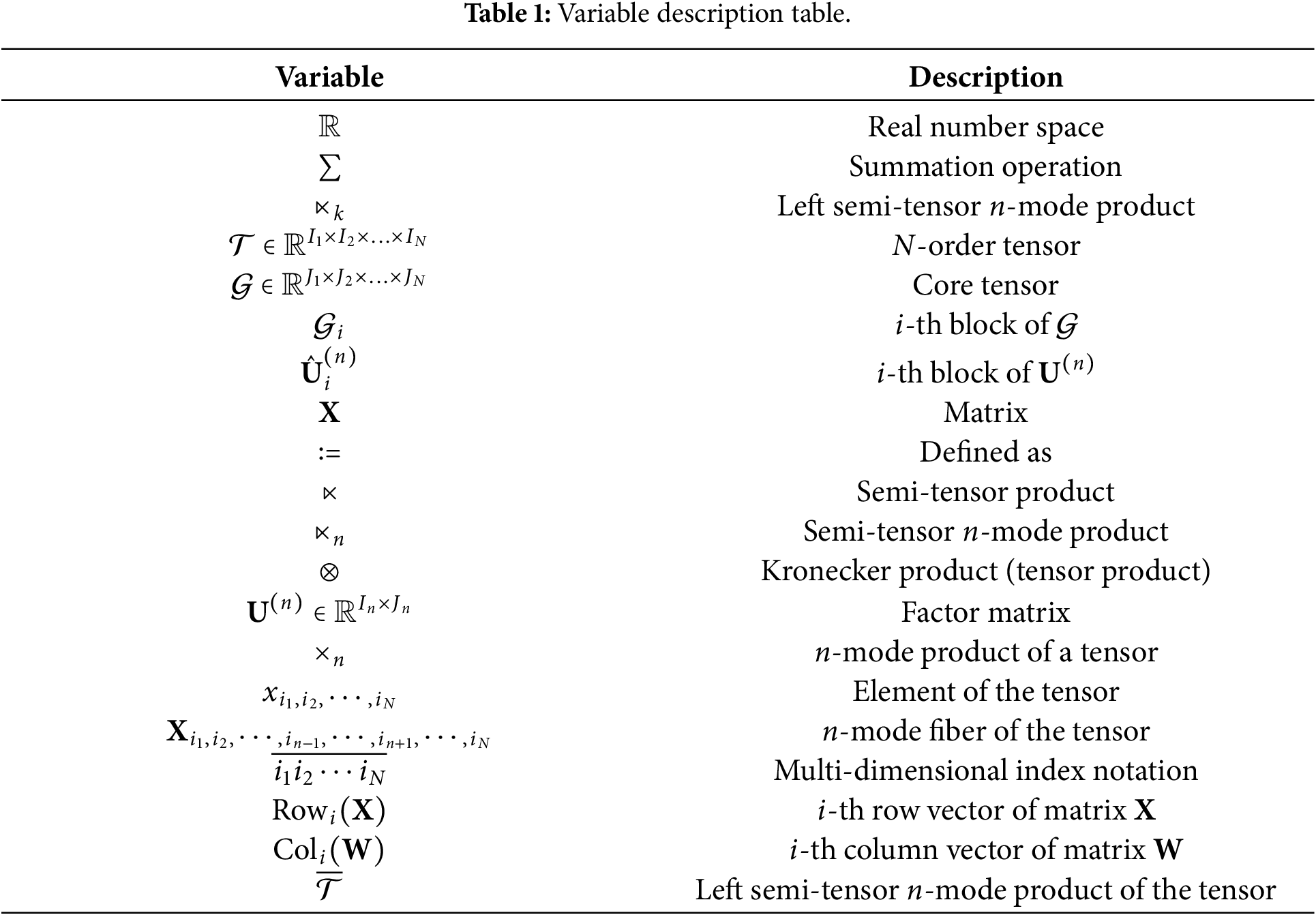
This section presents essential background on STP [8,31,32] and the pertinent tensor theory, forming the foundation of the proposed method. Variable Description is shown in Table 1.

Definition 1 (Kronecker product): Given two tensors 𝒳∈RI1×I2×…IN and 𝒴∈RJ1×J2×…JN, their Kronecker product yields a new tensor 𝒵∈RI1J1×I2J2×…×INJN, defined as

zi1j1¯,i2j2¯,⋯,iNjN¯=xi1,i2,⋯,iNyj1,j2,⋯,jN.(1)

This operation is denoted as 𝒵=𝒳⊗𝒴.

Definition 2 (Left semi-tensor product): For two matrices A∈Rm×n and B∈Rp×q, let t=lcm⁡(n,p) be the least common multiple of n and p. The left semi-tensor product, denoted by ⋉, is defined as

A⋉B=(A⊗It/n)(B⊗It/p),(2)

where A⋉B∈R(m⋅t/n)×(t/p⋅q), ⊗ is the Kronecker product, and It/n, It/p are identity matrices.

Example 1:

A=[1−12010],B=[1011].

lcm⁡(3,2)=6.

A⋉B=(A⊗I2)(B⊗I3)=[12−1020−112−102001000100100].

Based on the general definition, the dimensional relationship between A and B can be categorized into three cases:

(i)   If n=p, then A and B have an equal dimensional relationship.

(ii)   If n=tp or nt=p for some t∈Z+, then A and B have a multiple dimensional relationship. When n=tp, we write A≻tB; when nt=p, we write A≺tB.

(iii)   Otherwise, A and B have an arbitrary dimensional relationship.

Definition 3 (Semi-tensor product of vectors):

(i)   Let X∈Rtp be a row vector and Y∈Rp be a column vector (i.e., X≻tY). Partition X into p equal parts: X=(X1,…,Xp) with Xi∈Rt, i=1,…,p. Define

X⋉Y:=∑i=1pXiyi∈Rt.(3)

(ii)   Let X∈Rn be a row vector and Y∈Rnt be a column vector (i.e., X≺tY). Partition Y into n equal parts: Yi∈Rt, i=1,…,n. Define

X⋉Y:=∑i=1nxiYi∈Rt.(4)

(iii)   For matrices A∈Rm×n and B∈Rp×q with A≻tB (or A≺tB), the semi-tensor product is defined entrywise as

A⋉B=[Row1⁡(A)⋉Col1⁡(B)⋯Row1⁡(A)⋉Colq⁡(B)Row2⁡(A)⋉Col1⁡(B)⋯Row2⁡(A)⋉Colq⁡(B)⋮⋱⋮Rowm⁡(A)⋉Col1⁡(B)⋯Rowm⁡(A)⋉Colq⁡(B)].(5)

Definition 4 (Tensor n-mode multiplication): Given a tensor 𝒳∈RI1×I2×⋯×IN and a matrix A∈RK×In, the n-mode product of 𝒳 with A produces a new tensor 𝒴∈RI1×⋯×In−1×K×In+1×⋯×IN defined by

yi1,…,in−1,k,in+1,…,iN=∑in=1Inxi1,…,in,…,iNak,in.(6)

This operation is denoted as 𝒴=𝒳×nA. A tensor diagram of n-mode multiplication is shown in Fig. 1.

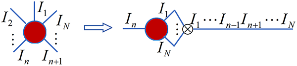
Figure 1: Tensor diagram of tensor n-mode multiplication.

Definition 5 (Tucker decomposition): Given a tensor 𝒳∈RI1×I2×⋯×IN, the Tucker decomposition factorizes it into a core tensor 𝒢∈RJ1×J2×⋯×JN (with Jn≤In, 1≤n≤N) and N factor matrices Un∈RIn×Jn:

𝒳=𝒢×1U1×2U2⋯×NUN.(7)

Here, ×n denotes the n-mode product, and (J1,J2,…,JN) is called the multilinear rank of the tensor.

4  Methodology Introduction

In this section, we first outline the framework of the proposed model, then present the Semi-Tensor Product-based Block Term Decomposition (STP-BTD). Finally, by incorporating multimodal multilinear pooling, we introduce the Semi-Tensor Product-based Block Term Decomposition of Multilinear (STP-BTDM) pooling method.

4.1 Model Structure

Fig. 2 illustrates the overall architecture of the STP-BTDM method. The vectors x1∈RI1, x2∈RI2, and x3∈RI3 are obtained by processing unimodal inputs (e.g., text, video, and audio) through their corresponding sub-networks fl, fa, and fv, respectively. These modalities are then fused using the proposed STP-BTDM pooling method to produce an output representation y for downstream prediction tasks. The detailed procedure within the dashed box in the figure is described in the following subsections.

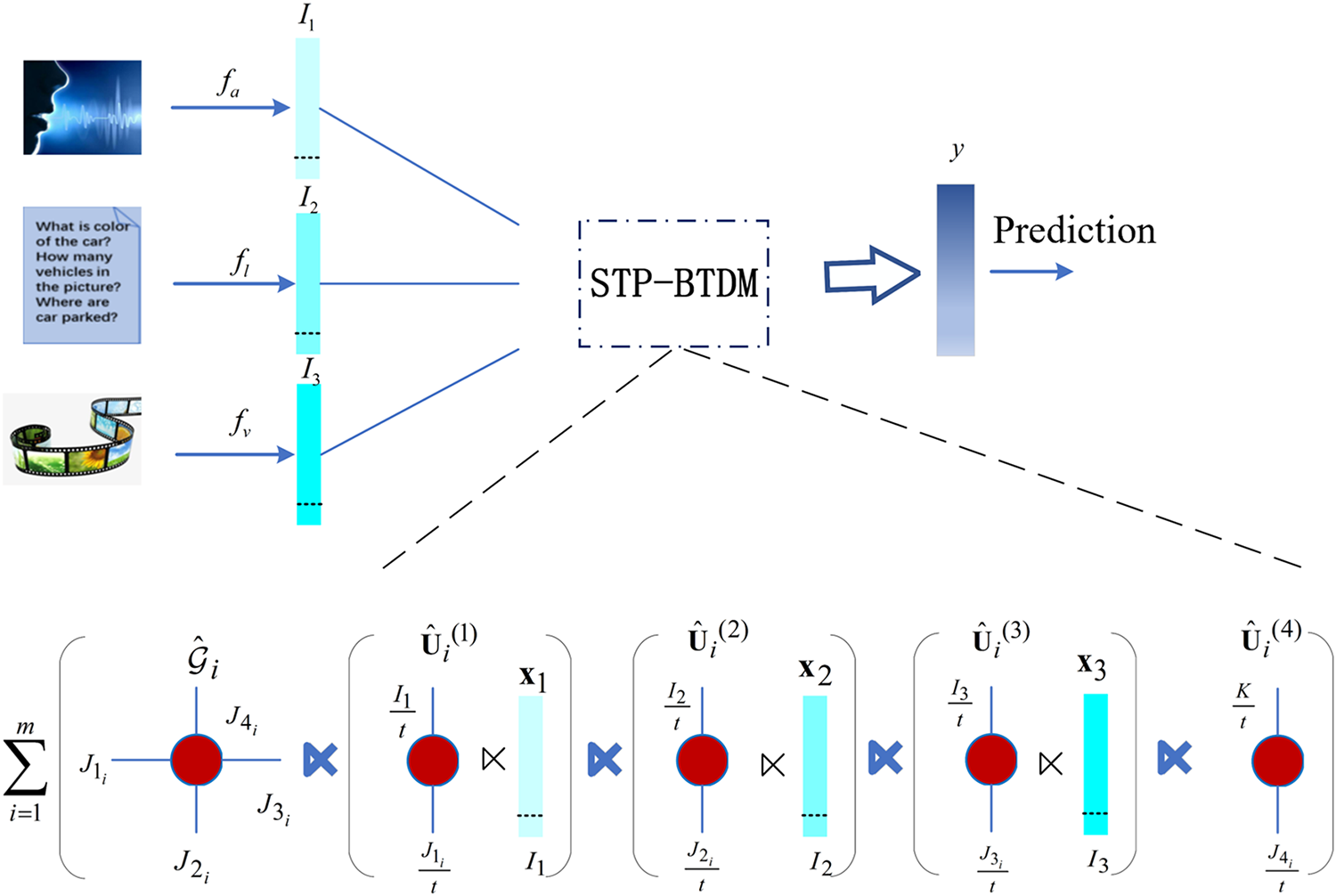
Figure 2: The model structure of STP-BTDM method.

4.2 Block Term Decomposition

Tucker decomposition has been introduced in Section 3 (Notations and Preliminaries). In its standard form, Tucker decomposition imposes no constraints on the core tensor. However, to ensure high decomposition accuracy, the core tensor dimensions are typically set to relatively large values, leading to a large number of parameters. To address this issue, a diagonal block constraint is imposed on the core tensor, effectively reducing its dimensionality. Lathauwer proposed the Block Term Decomposition (BTD) of a tensor to minimize the number of parameters and limit model complexity. The BTD can be expressed as

𝒯=∑i=1M𝒢i×1Ui(1)×2Ui(2)…×NUi(N).(8)

Unlike standard Tucker decomposition, in BTD the core tensor 𝒢∈RJ1×J2×…×JN is block-diagonal when the original tensor 𝒯∈RI1×I2×…×IN undergoes block-term decomposition, as illustrated by the red box in Fig. 3 (using a third-order tensor as an example). The core tensor 𝒢 is partitioned into smaller tensor blocks, where 𝒢i denotes the i-th block of 𝒢. Consequently, 𝒢 can be represented as a block-diagonal tensor: 𝒢=diag⁡(𝒢1,…,𝒢i,…,𝒢M), with M indicating the number of blocks. Correspondingly, the factor matrix U(n)∈RIn×Jn (n=1,2,…) is also divided into blocks: U(n)=[U1(n),…,UI(n),…,UM(n)], as shown in the green box in Fig. 3 (again for a third-order tensor). Then the tensor block-term decomposition can be expressed as Eq. (8).

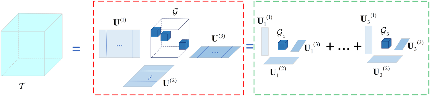
Figure 3: Decomposition of block terms of a third-order tensor. The uncolored regions of the core tensor 𝒢 in the red box indicate zero entries.

4.3 Block-Term Decomposition Based on Semi-Tensor Product (STP-BTD)

In this subsection, we replace the conventional matrix product with the semi-tensor product and introduce the STP-Tucker decomposition format. This format offers a more streamlined low-rank tensor structure by decomposing a tensor into the semi-tensor product of a core tensor and factor matrices along each mode. It is represented as

𝒯=𝒢^⋉1U^(1)⋉2U^(2)…⋉NU^(N),𝒯∈RI1×I2×…×IN,(9)

where ⋉n denotes the left semi-tensor n-mode product, 𝒢^∈RJ1×J2×…×JN is the core tensor, and U^(n)∈RJnt×Int (n=1,2,…,N) are the factor matrices.

Consequently, the left semi-tensor n-mode product of the core tensor 𝒢^ with a factor matrix U^(n) is given by

𝒯¯=𝒢^⋉nU^(n).(10)

We then apply the STP-Tucker decomposition form to block-term decomposition, yielding the Semi-Tensor Product-based Block Term Decomposition (STP-BTD). The detailed procedure is as follows. The core tensor 𝒢^ is divided into smaller tensor blocks, and 𝒢^ itself is block-diagonal:

𝒢^=diag⁡(𝒢^1,…,𝒢^i,…,𝒢^M),

where M is the number of blocks. The factor matrices are partitioned accordingly:

U^(1)=[U^1(1),…,U^i(1),…,U^M(1)],U^(2)=[U^1(2),…,U^i(2),…,U^M(2)],  ⋮U^(N)=[U^1(N),…,U^i(N),…,U^M(N)].

with

U^i(1)∈RJ1it×I1t,U^i(2)∈RJ2it×I2t,…,U^i(N)∈RJNit×INt.

Fig. 4 visually illustrates the computation process of STP-BTD. Hence, Eq. (9) can be rewritten as

𝒯=∑i=1M𝒢^i⋉1U^i(1)⋉2U^i(2)…⋉NU^i(N).(11)

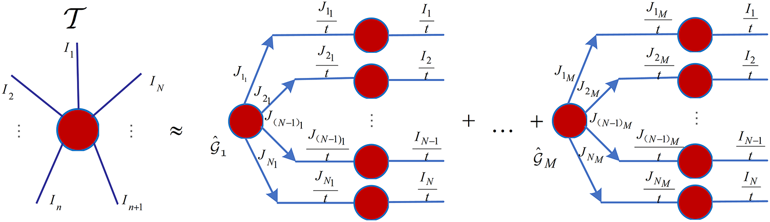
Figure 4: Visual representation of the STP-BTDM method.

The relationship between the number of blocks and the core tensor dimensions is given by

∑i=1MJ1it=J1t,∑i=1MJ2it=J2t,…,∑i=1MJNit=JNt.(12)

In light of Eqs. (11) and (12), each element of the original tensor 𝒯 of order N can be expressed as a function involving the STP-based core tensor blocks and factor matrices. The core tensor resides in a significantly smaller space composed of STP block-diagonal tensors, which are not only simple but also expressive, as they strike a balance between dense and diagonal tensors.

4.4 Multimodal Decomposition Multilinear Pooling Model

The bilinear pooling model takes a pair of vectors x1∈RI1 and x2∈RI2 as inputs and computes their interaction via the tensor product, resulting in a projection into a K-dimensional space:

y=𝒯×1x1×2x2,(13)

where y∈RK. Each component of y is given by a quadratic expression of the input variables:

yk=∑i=1I1∑j=1I2𝒯ijk⋅x1i⋅x2j,k∈[1,K].(14)

Thus, the bilinear pooling model is completely determined by its associated tensor 𝒯∈RI1×I2×K. Eq. (14) illustrates the advantage of leveraging complex interactions among feature dimensions to capture shared semantic aspects of multimodal features. We therefore extend bilinear pooling to multilinear pooling to enhance the expressive power of fused features:

y=𝒯×1x1×2x2×3x3,(15)

where y∈RK is the fused feature vector. Here, x1∈RI1, x2∈RI2, and x3∈RI3 are unimodal input vectors from three different modalities, which collectively project to a K-dimensional tensor 𝒯∈RI1×I2×I3×K. With three input modalities, the weight tensor 𝒯 is naturally a fourth-order tensor, where the fourth dimension corresponds to the output size K. The element-wise expression is:

yk=∑i=1I1∑j=1I2∑o=1I3𝒯ijok⋅x1i⋅x2j⋅x3o,k∈[1,K].(16)

In this section, we consider the weight tensor to be of order 4 and apply Tucker decomposition (TD):

𝒯=𝒢×1U(1)×2U(2)×3U(3)×4U(4),(17)

where 𝒢∈RJ1×J2×J3×J4, U(1)∈RI1×J1, U(2)∈RI2×J2, U(3)∈RI3×J3, U(4)∈RK×J4, and ×n (n=1,2,3,4) denotes the n-mode product (also called the modular n product). Eq. (17) indicates that the weight tensor 𝒯 depends on a finite set of parameters for all i∈[1,I1], j∈[1,I2], k∈[1,I3], o∈[1,K]:

𝒯[i,j,k,o]=∑l=1J1∑m=1J2∑n=1J3∑p=1J4𝒢[l,m,n,p]U(1)[i,l]U(2)[j,m]U(3)[k,n]U(4)[o,p].(18)

The weight tensor 𝒯 is parameterized by the Tucker decomposition in Eq. (17), and the multimodal multilinear pooling method is adopted as:

y=𝒯×1x1×2x2×3x3=(((𝒢×1(x1TU(1)))×2(x2TU(2)))×3(x3TU(3)))×4U(4).(19)

Let y~=((𝒢×1(x1TU(1)))×2(x2TU(2)))×3(x3TU(3)). The matrices U(1), U(2), and U(3) project the unimodal vectors x1, x2, and x3 into spaces of dimensions J1, J2, and J3, respectively, which directly affect the modeling complexity of each modality. Define x~1=x1TU(1)∈RJ1, x~2=x2TU(2)∈RJ2, and x~3=x3TU(3)∈RJ3; their interactions are modeled by the core tensor 𝒢. The core tensor learns from all correlations x~1[i]x~2[j]x~3[k] and projects them onto a vector y~ of dimension J4, which determines the complexity of inter-modal interactions. Then y=y~×4U(4); in other words, the multilinear interaction representation y~ is mapped to the K-dimensional output space via U(4). To achieve a K-dimensional output y=[y1,…,yK], the tensor 𝒯 must be learned. Unfortunately, 𝒯 has high dimensionality and a large number of parameters, leading to substantial computational and memory overheads.

4.5 Semi-Tensor Product-Based Block Term Decomposition of Multilinear Pooling (STP-BTDM) Method

In contrast to STP-MFM which relies on low-rank factorized pooling, the proposed STP-BTDM leverages block-term decomposition under the semi-tensor product framework to achieve a block-diagonal core tensor, thereby enabling modality-specific subspace learning (where each modality is assigned to an independent block of the core tensor) and capturing fine-grained multilinear interactions with reduced parameter complexity.

Based on the decomposition of the weight tensor 𝒯 discussed above, and noting that the dimensions of the input vectors x1, x2, x3 have multiple relations with the matrices U^(1), U^(2), U^(3), we apply the semi-tensor product. We project the input vectors into the spaces of dimensions J1, J2, J3 via U^(1), U^(2), U^(3) as x1T⋉U^(1), x2T⋉U^(2), and x3T⋉U^(3). Consequently, Eq. (19) can be rewritten as:

y=(𝒢^⋉1(x1T⋉U^(1)))⋉2(x2T⋉U^(2))⋉3(x3T⋉U^(3))⋉4U^(4).(20)

Let x^1=x1T⋉U^(1)∈RJ1t, x^2=x2T⋉U^(2)∈RJ2t, and x^3=x3T⋉U^(3)∈RJ3t. These projected features are then fused via the semi-tensor product with the block super-diagonal tensor 𝒢^, which itself is parameterized in the semi-tensor framework. This process encodes the complete multilinear interactions among x1, x2, and x3 into an intermediate representation, which is subsequently projected to the output space y.

Furthermore, combining Eqs. (11) and (20), the STP-BTDM expression is given by:

y=∑i=1M((𝒢^i⋉1(x1T⋉U^i(1)))⋉2(x2T⋉U^i(2)))⋉3(x3T⋉U^i(3))⋉4U^i(4).(21)

The tensor 𝒢i^ combines the size J1t, J2t and J3t blocks from x1^, x2^ and x3^ together to generate a vector of J4t size:

zi=𝒢^i⋉1x^1iJ1t:(i+1)J1tT⋉2x^2iJ2t:(i+1)J2tT⋉3x^3iJ3t:(i+1)J3tT.(22)

Here x^i:j denotes the sub-vector of x^ from index i to j−1 (inclusive), whose dimension is j−i. And finally, all of the vectors z∈RJ4t are connected to from zi, which is z={z1,…,zi}. The final prediction vector is y=z⋉U^(4)∈RK.

In light of Eqs. (20) and (21), the multilinear space 𝒢^i is decomposed into several subspaces. The input audio, video, and text features are projected into each subspace via the corresponding projection matrices U^i(1), U^i(2), U^i(3), and the dimension of the projected features matches the size of the respective tensor block 𝒢^i. This sparse structure allows the multilinear model to capture distinct third-order interactions in different subspaces. Algorithm 1 outlines the STP-BTDM procedure.

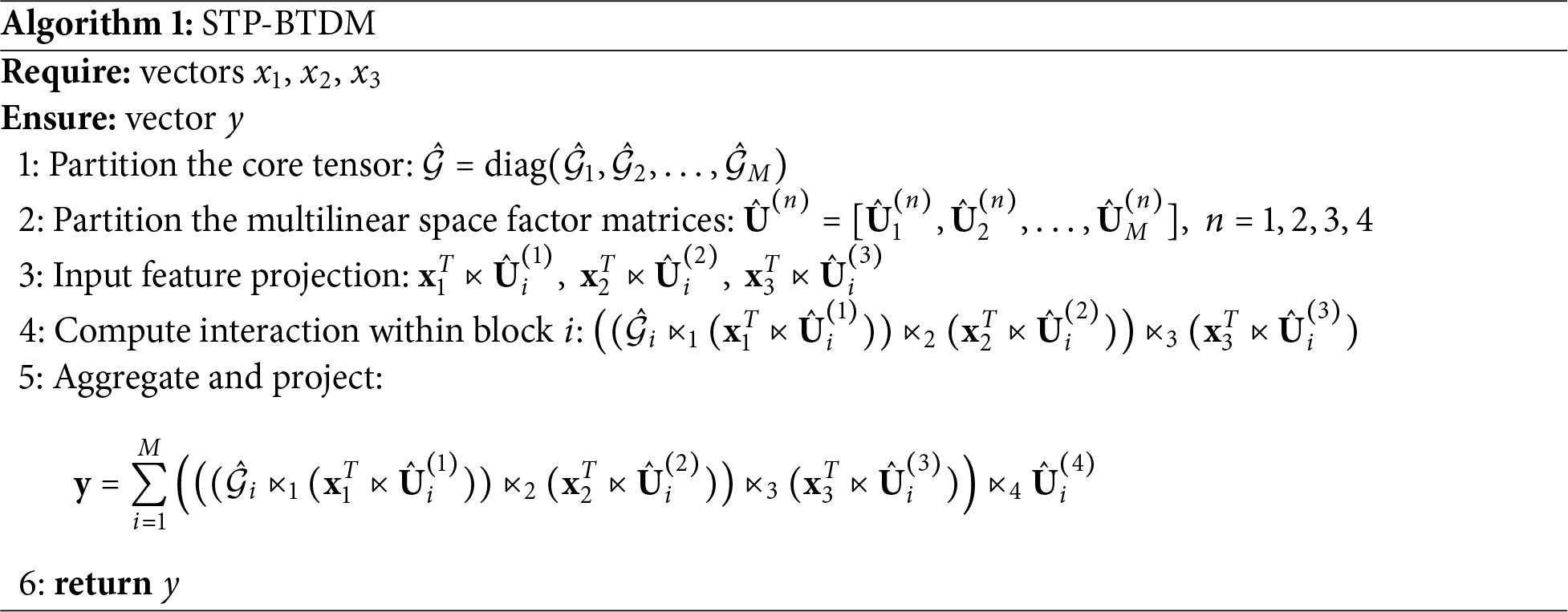
The algorithm captures the interaction between the tensor block 𝒢^i and the projection matrices U^i(1), U^i(2), U^i(3), U^i(4). The text, video, and audio features x1, x2, x3 are projected into the spaces defined by U^i(1), U^i(2), U^i(3) for multilinear operations. Subsequently, the core tensor 𝒢^i captures comprehensive third-order interactions across the three modalities and consolidates them into a unified integrated feature, akin to performing many fine-grained multilinear operations in different feature subspaces. Finally, the integrated feature is projected by U^i(4). Hence, the dimension of the projected feature is determined by the block tensor dimensions. The advantage of this method is that it obtains interactions of corresponding feature vectors within the tensor block space. The introduction of STP eliminates the dimensional consistency requirement in matrix multiplication, leading to a more compact architecture and reduced memory usage. More importantly, STP preserves sequential and spatial information through block-level operations, thereby enhancing the representation of intra-modality correlations across diverse modalities. As discussed in Section 1, these properties—global sparsity with local density, modality-specific block independence, and fine-grained subspace interactions—fundamentally distinguish STP-BTDM from prior factorized multilinear approaches such as STP-MFM.

Fig. 2 provides a visual illustration of STP-BTDM, and Algorithm 1 details its computational steps.

5  Experimental Setting

5.1 Datasets Introduction

To validate the performance of the STP-BTDM method, two commonly used datasets, CMU-MOSI [33] and IEMOCAP [34], were selected to verify the multi-modal sentiment analysis tasks. Both datasets consist of three modalities: text, video and audio data. Here are descriptions of the CMU-MOSI and IEMOCAP datasets, respectively:

The CMU-MOSI dataset comprises 93 randomly selected YouTube vlog videos featuring 89 independent speakers. One significant advantage of these videos is their diversity and inclusion of ambient noise, as they are captured in various environments using a wide range of recording equipment, from professional microphones and cameras to more basic devices. Among the 41 female and 48 male speakers, ages ranged from 20 to 30 years old. On average, each video contains 23.2 opinion segments (subjective clips), with each segment averaging approximately 4.2 s in length. In total, the dataset contains 2198 subjective video clips, each annotated with an emotional intensity score ranging from strongly negative to strongly positive. Distinguished by carrying an opinion, belief, thought, feeling, emotion, goal, evaluation, or judgment, subjective annotation produced 2199 subjective fragments, each of which was labeled with an emotional intensity definition ranging from strongly negative to strongly positive. These statements were manually labeled as a continuous opinion score between [−3, 3] and each video was labeled by five workers and finally averaged, where −3/+3 represented strong negative/positive emotions. This dataset provides manual annotations of facial expressions and head gestures to study the relationship between words and non-verbal cues. Since hands are not often seen in the video, we focused on four primary facial/head gestures: smile, frown, nod, and shake. All experiments in this data are done in the speaker-independent frame and each speaker’s opinion paragraph will only appear in one of the training, validation, or test sets.

The IEMOCAP dataset was captured at the Robert Zemeckis Center within the John C. Hench Department of Animation and Digital Arts at the University of Southern California. Data was recorded using the VICON Motion Capture system, comprising six cameras positioned approximately one meter from the subjects. The database contained a total of approximately 12 h of data, comprising 151 dyadic dialogues, with video, audio, and motion capture recordings of both speakers in each session. Each session required performances by a female and a male actor. Used to capture the face, hand and head movements. It is recorded in two formats: one involves dramatic performances designed to convey specific emotions such as happiness, anger, sadness, frustration and neutral states. The other is improvisation, which requires the actor to improvise based on a hypothetical scenario to trigger a specific emotion. The dataset contains 151 dyadic sessions (each with two speakers, recorded from two perspectives), totaling 302 video recordings, with each segment annotated for 9 emotion categories. In this experiment, four emotion categories (neutral, happy, sad and angry) are selected for the binary classification task research, in which the training set comprises 2717 data, the validation set contains 798 data points, and the test set includes 938 data.

Both datasets have been de-identified and made publicly available by their original creators for academic research purposes. The data segmentation of the training set, validation set and test set is shown in Table 2. In both the training and test datasets, speakers do not overlap.

For IEMOCAP, the training, validation, and test sets contain 2717, 798, and 938 samples, respectively, as described in the text above. The CMU-MOSI dataset is split into 1284 training, 229 validation, and 686 test samples.

5.2 Features

The aforementioned datasets include three modalities: text, video and audio. We use P2FA [35] for word alignment to achieve cross-modal alignment. The audio and video features are extracted by averaging their values across the duration of the spoken words.

Text features extraction uses the GloVe (Global Vectors for Word Representation) model [36] to vectorize spoken text words, the semantic similarity between two words can be calculated through operations on vectors such as Euclidean distance or cosine similarity. Long Short-Term Memory (LSTM), an improved model of RNN, can learn long-term dependent information and avoid the gradient disappearance problem of RNN. The GloVe model adopts AdaGrad’s gradient descent algorithm during training. The value of α is 0.75, the value of x(max) is 100, the learning rate is set to 0.05 and the output feature dimension is fixed to 300 dimensions. After 50 iterations until convergence, two vectors are finally learned. In this paper, the sum of the two is chosen as the final word vector and the resulting word vector with dimension (20, 300) is taken as the input of the text embedding subnetwork.

Audio features extraction uses the COVAREP acoustic analysis framework [37] to derive a set of acoustic features for use as input to the speech embedding subnetwork. In this paper, the input dimension is set as (Ta, 74), where Ta represents the number of segmented frames of the audio segment and 74 represents the number of acoustic features. The COVAREP acoustic analysis framework includes 12 MFCCs, pitch tracking, noise segmentation features using additive noise-robust summation of residual harmonics, parameters for voice source (glottal inverse filtering estimation based on GCI-synchronous IAIF), peak slope parameters and maximum dispersion entropy features. The framework extracts different features of the human voice and has been shown to correlate these vocal features with emotion.

Visual features extraction employs the FACET facial expression analysis framework to extract indicators [38] for seven basic emotions (anger, contempt, disgust, fear, joy, sadness and surprise) and two higher emotions (frustration and confusion). Facial action units [39] capturing detailed facial muscle movements were also extracted using FACET. OpenFace was utilized to estimate head position and head rotation, and extract 68 facial landmark positions per frame. Because the information extracted from the video using FACET is rich, the use of deep neural networks will be sufficient to produce meaningful visual modal embeddings. Therefore, a deep neural network with 32 ReLU units with three hidden layers and weights Wv is used. Empirical findings indicate that increasing the model depth or the number of neurons per layer does not necessarily improve visual performance. Each video feature has a dimension of 35.

5.3 Baseline Model

This paper employs the Tensor Fusion Network (TFN), Low-rank Multi-modal Fusion (LMF), and Semi-Tensor Product-based Multi-modal Factorized Multilinear pooling (STP-MFM) as baseline methods, representing the current state-of-the-art approaches for tensor-based methodologies. Compare the proposed STP-BTDM method with Baseline models on two different multimodal datasets for emotion analysis.

Tensor Fusion Network (TFN) [5] achieves fusion by constructing multidimensional tensors that capture interactions across unimodal, bimodal and trimodal data from three modalities. It mathematically corresponds to the outer product between visual, audio, and text embedding. However, when the data volume increases, the computational complexity also rises.

The Low-rank Multi-modal Fusion (LMF) [22] conducted tensor factorization using uniform low-rank for multi-modal fusion. By using low-rank matrix decomposition of weights, LMF changes the process of TFN’s pre-tensor outer product and then goes through the FC (Full Connection) layer into a multi-dimensional dot product for each modality, which can be viewed as the aggregation of outcomes from multiple low-rank vectors, effectively reducing the model’s parameter count.

Semi-Tensor Product-based Multi-modal Factorized Multilinear pooling (STP-MFM) [11] leverages the STP to achieve adaptable and condensed tensor decompositions using reduced factor matrices, which project the input features into a compact multilinear space. This method allows connecting factors of differing dimensionalities through the semi-tensor mode product, eliminating the need for dimension consistency found in traditional matrix multiplication. Consequently, STP-MFM represents information in a more condensed structure, optimizing memory usage.

In addition to these tensor-based baselines, we further compare STP-BTDM with two recent state-of-the-art methods that represent the current mainstream directions in multimodal sentiment analysis:

Multimodal Transformer (MulT) [40] employs cross-modal attention mechanisms to capture long-range dependencies across modalities without requiring strict temporal alignment. It has been widely adopted as a strong transformer-based benchmark in the field.

MISA (Modality-Invariant and -Specific Representations) [41] learns both modality-invariant and modality-specific features through disentanglement, achieving superior performance by reducing modality gaps while preserving useful modality-specific information. We include this method as a representative of advanced representation learning for multimodal fusion.

5.4 Model Architecture

Utilize the GloVe model and select Long Short-Term Memory (LSTM) networks to extract features from text modalities. Employ the COVAREP acoustic analysis framework and choose a straightforward two-layer feedforward neural network to extract features from audio modalities. Use the FACET framework, opting for a two-layer feedforward neural network to obtain features from video modalities. The initial lengths of the audio, video and text features are 74, 35 and 300, correspondingly. For feature extraction, we consider candidate lengths from the following ranges: [16, 32, 64] for audio, [16, 32, 64] for video, and [32, 64, 128] for text. To ensure reproducibility and a fair comparison across all models, we fix the feature extraction lengths for each modality after a preliminary hyperparameter search. Specifically, we select 64 for audio, 64 for video, and 128 for text, and these fixed lengths are used consistently for all baseline models and STP-BTDM in the final experiments. No random selection of feature dimensions occurs during training iterations.

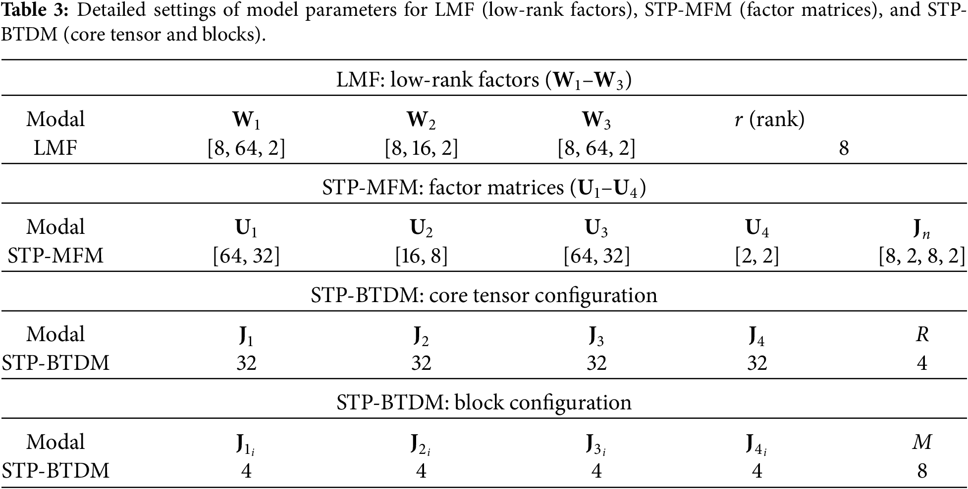
In the STP-MFM model, we set the dimensions of the factor matrices to [64, 32], [16, 8], [64, 32] and [2, 2]. The core tensor has dimensions of [8, 2, 8, 2]. In the STP-BTDM model, we configure the core tensor size to J1=J2=J3=J4=32, with a rank R=4, and establish 8 blocks within the core tensor, indicating that each block size is J1i=J2i=J3i=J4i=4. We designated the core tensor size as 32 with a rank of 4, and organized the core tensor into 8 blocks, where each block has a size of 4. The specific configurations of weight factors, core tensors and blocks for each modality are detailed in Table 3.

5.5 Evaluation Metrics

In order to evaluate the performance of the proposed method, regression and classification evaluation tasks were performed in the experiment. The classification task was applied to both datasets, while the regression task specifically targeted the CMU-MOSI dataset. For binary classification, binary classification accuracy (Acc-2) and weighted average F1 value (F1) score were used as performance evaluation metrics. For the other group, accuracy was evaluated using the 7-class accuracy metric (Acc-7). For the regression task, performance was assessed using the mean absolute error (MAE) and the correlation (Corr). Except for MAE, higher values of these metrics indicate better outcomes.

5.6 Training Configuration

The STP-BTDM approach is realized using the PyTorch framework, which is open-source. We select hyperparameters via grid search, determining them based on the model’s performance on the validation set. For optimization, we employ the Adam optimizer with an initial learning rate of 0.0003 and a batch size of 32. To prevent overfitting, we apply two separate regularization strategies: L2 regularization (weight decay) with a coefficient of 0.01, and Dropout with a retention probability of 0.15.

5.7 Reproducibility and Statistical Significance

To ensure the reproducibility and reliability of our experimental results, we provide the following detailed settings.

Random seeds and repeated runs.

All experiments are conducted with five independent runs using different random seeds: 42, 123, 2024, 456, and 789. For each run, the dataset splits remain fixed, but model parameters are randomly initialized. We report the mean and standard deviation (mean ± std) for each evaluation metric across the five runs.

Hardware and software environment.

All models are trained and evaluated on a single server equipped with an NVIDIA RTX 3090 GPU (24 GB memory), an Intel Core i9-10900K CPU, and 64 GB of RAM, running Ubuntu 20.04 LTS. The implementation is based on PyTorch 1.12.0 with CUDA 11.6.

Early stopping and learning schedule.

We employ early stopping with a patience of 10 epochs on the validation loss; the model checkpoint that yields the lowest validation loss is selected for final testing. The Adam optimizer is used with an initial learning rate of 3×10−4, and a StepLR scheduler reduces the learning rate by half every 15 epochs until convergence. The maximum number of training epochs is set to 100, but early stopping typically terminates training within 40–50 epochs.

Baseline implementation details.

For TFN [5] and LMF [22], we use the official source code provided by the original authors and tune hyperparameters on the validation set according to their recommended ranges. For STP-MFM [11], we use the implementation from the same research group. For the newly added baselines, MulT [40] and MISA [41], we use the publicly available implementations with the hyperparameters suggested in their original papers. All baselines are re-run under the identical random seed and hardware settings described above to ensure a fair comparison. The specific hyperparameter configurations for each baseline are listed in Table 3.

Statistical significance testing.

We perform paired t-tests between STP-BTDM and each baseline on the test set results from the five independent runs to determine whether the observed differences are statistically significant (p<0.05). The significance markers are included in Tables 4 and 5.

6  Results

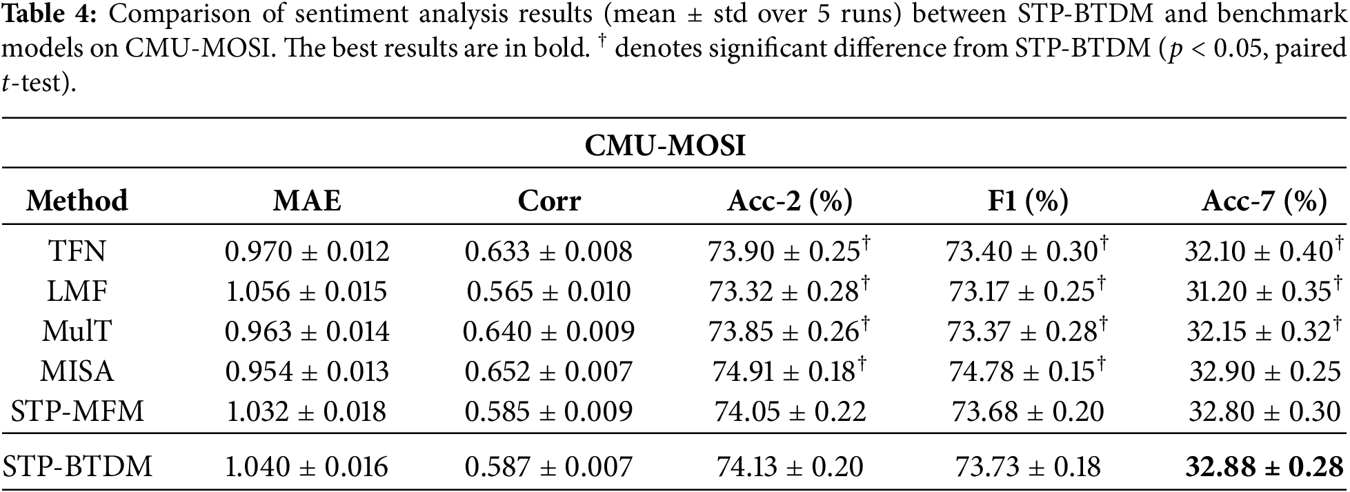
We conducted comparisons between our model and TFN, LMF and STP-MFM on tasks involving sentiment analysis. To ensure fairness, all three models were executed under identical environmental conditions.

6.1 Comparison with the Baseline Model

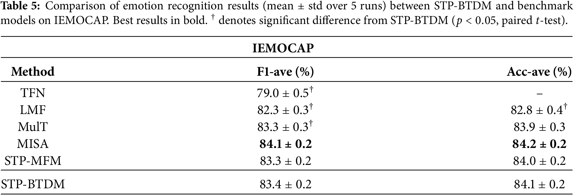
To assess the performance of STP-BTDM in emotion analysis tasks, it is compared with three benchmark models in some common evaluation indicators. Table 4 is the comparison of sentiment analysis results between STP-BTDM and the benchmark model on CMU-MOSI. Table 5 is the comparison of emotion recognition results between STP-BTDM and the benchmark model on the IEMOCAP dataset.

The results are detailed in Tables 4 and 5.

From the experimental results in Table 4 on CMU-MOSI, the proposed STP-BTDM model achieves the best Acc-7 (32.88±0.28%) among all compared methods, outperforming MISA by 0.02% and exceeding LMF by 1.68%. The binary classification accuracy is 74.13±0.20%, with an F1 score of 73.73±0.18%. Compared with STP-MFM, the improvements are 0.08±0.02% in Acc-2, 0.05±0.02% in F1, and 0.08±0.03% in Acc-7. Paired t-tests indicate that these differences are not statistically significant (p>0.05), suggesting that STP-BTDM performs comparably to STP-MFM on this dataset while offering structural advantages in sparsity and modality-specific modeling. However, STP-BTDM significantly outperforms TFN, LMF, and MulT (p<0.05) across most metrics.

On IEMOCAP, as shown in Table 5, MISA achieves the highest average F1 (84.1±0.2%) and accuracy (84.2±0.2%), slightly outperforming STP-BTDM (83.4±0.2% and 84.1±0.2%). Nevertheless, STP-BTDM remains highly competitive: it surpasses all tensor-based baselines (TFN, LMF, and STP-MFM) and performs on par with MISA while requiring a much more compact architecture and a globally sparse yet locally dense tensor structure. The improvement over STP-MFM is 0.1±0.1% in both metrics, which is not statistically significant (p>0.05); however, the gains over LMF and TFN are significant (p<0.05).

It is worth noting that MISA achieves slightly better performance on IEMOCAP, but it employs a more complex disentanglement framework with additional loss terms and adversarial training. In contrast, STP-BTDM achieves comparable results with approximately 1.1×105 parameters (about 1/11 of TFN), and its block-diagonal core tensor enables explicit modality-specific subspace modeling and fine-grained multilinear interactions. Furthermore, on the more challenging 7-class sentiment classification (Acc-7) of CMU-MOSI, STP-BTDM outperforms all methods including MISA, demonstrating its particular strength in fine-grained discrimination.

Overall, the expanded comparisons with transformer-based (MulT) and disentanglement-based (MISA) methods demonstrate that STP-BTDM is not only competitive with traditional tensor fusion approaches but also remains relevant when compared with recent state-of-the-art models. While MISA shows slightly higher accuracy on IEMOCAP, STP-BTDM offers a unique combination of advantages: (1) the globally sparse yet locally dense tensor structure enables efficient parameter utilization; (2) the block-diagonal design provides explicit modality-specific subspace modeling; and (3) the semi-tensor product removes dimensional consistency constraints, offering greater flexibility in handling heterogeneous multimodal features. These properties make STP-BTDM a practical, interpretable, and efficient alternative to more complex fusion frameworks.

Fig. 5 shows the F1 scores of the proposed STP-BTDM model and three baseline models (TFN, LMF, and STP-MFM) for the recognition of Happy, Sad, Angry, and Neutral emotions on the IEMOCAP dataset. STP-BTDM has higher F1 values for all emotion recognition than the benchmark model. Emotions Happy, Sad and Angry all have higher F1 values, indicating that these three emotions are easier to recognize.

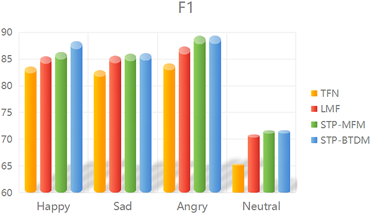
Figure 5: Comparison of F1 scores of TFN, LMF, STP-MFM and STP-BTDM in four emotion recognition methods. The horizontal coordinates are the four emotions: Happy, Sad, Angry and Neutral are happy, sad, angry and neutral and the vertical coordinates are F1 scores.

Fig. 6 shows the recognition accuracy of the proposed STP-BTDM model and three baseline models (LMF, STP-MFM, and STP-BTDM) for the four emotion categories. The results demonstrate that STP-BTDM consistently outperforms the baselines across all emotions. STP-BTDM was more accurate than the benchmark model in all emotions. In addition, the accuracy of almost every emotion recognition is high, except the neutral emotion recognition is poor on the whole, which may be because the model has a better effect on the features with obvious performance when capturing features, while it has a poor ability to capture the features with mixed or fuzzy boundaries.

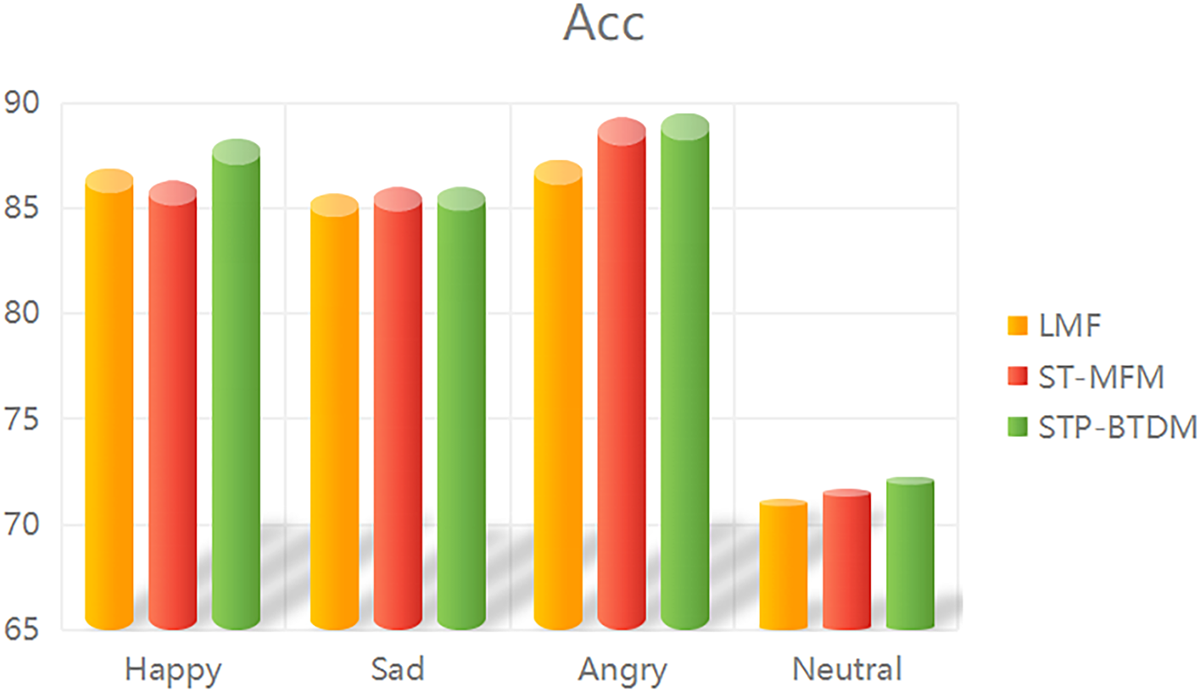
Figure 6: Comparison of Acc accuracy values of LMF, STP-MFM and STP-BTDM in four kinds of emotion recognition. The horizontal coordinate represents the four emotions: Happy, Sad, Angry and Neutral represent happy, sad, angry and neutral and the vertical coordinate represents the Acc accuracy value.

The results shown in Figs. 5 and 6 confirm the observations of Table 5. These experimental results show the necessity and effectiveness of the application of semi-tensor products in multi-modal information fusion. According to the characteristics of block term decomposition, the semi-tensor product is cleverly introduced and the multidimensional relationship between them is used to make the operation of block multiplication reasonably applied. In comparison to other mechanisms that employ point-by-point methodologies, it can better retain the time and space information of video, audio and text, better represent the intra-modal correlation and improve the fusion performance. Secondly, by introducing the block term decomposition of the proposed semi-tensor product, the characteristics of global sparse and local dense are reflected, which is exactly in line with the characteristics of neural networks and can better capture the correlation and complementarity between modes and promote the fusion of modes.

6.2 Ablation Experiment of the Influence of Block Diagonal Core Tensor on Model Performance

To investigate the impact of the block diagonal core tensor on model performance, an ablation experiment was conducted. The core tensor size was fixed at J1=J2=J3=J4=32, while the number of diagonal blocks varied from 1 to 16. As the number of diagonal blocks increased, the size of each block decreased accordingly. The core tensor 𝒢^ is small and a spatial block diagonal tensor. Block diagonal tensors are between dense tensors and diagonal tensors in complexity and are simple and expressive. Therefore, explicit sparsity is introduced into the multi-modal fusion method. We kept the size of each block 𝒢i^) constant and varied the number of diagonal blocks. Each block was set to J1i=J2i=J3i=J4i=4, with the number of diagonal blocks ranging from 1 to 16. As the number of blocks increased, the size of the core tensor also increased.

The result is shown in Fig. 7. Too many or too few blocks can cause performance degradation. For both Settings, a small number of blocks results in a dense kernel tensor, whereas a large number of blocks leads to a sparser kernel tensor. Selecting the appropriate number of blocks involves striking a balance between density and sparsity. Therefore, a configuration with a block number of 4 is considered in the prediction task.

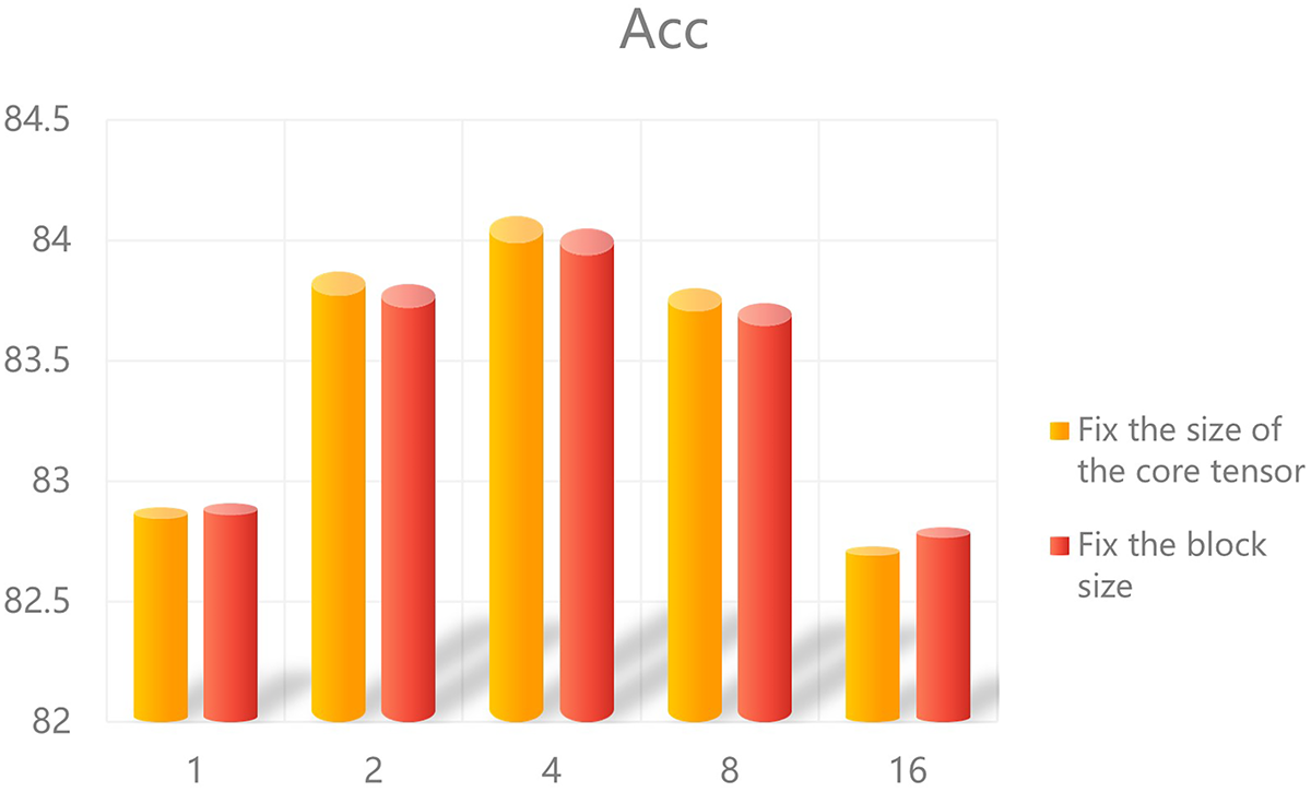
Figure 7: Influence of block diagonal core tensor on STP-BTDM model. Fixed the core tensor size and varied the number of blocks from 1 to 16; kept the block size constant and observed changes in the accuracy (ACC) values.

In multi-modal fusion, learning becomes very difficult due to the different interactions of different aspects that need to be captured by a global large tensor. On the contrary, the proposed method assigns each mode to a single block within the block diagonal kernel, enabling the core tensor’s sparsity to ensure independence among different blocks during training. This approach effectively simplifies the learning of multilinear interactions.

The number of the block tensor controls the dimensionality of the projection feature. This method is advantageous because it allows for capturing interactions among the respective feature vectors within the tensor block space.

6.3 The Influence of the Hyperparameter Setting on Model Performance

In the experiment, the influence of the setting of hyperparameter “t” on sentiment recognition performance was studied by fixing other parameters. The comparison of sentiment recognition performance results under different “t” values is observed in Table 6.

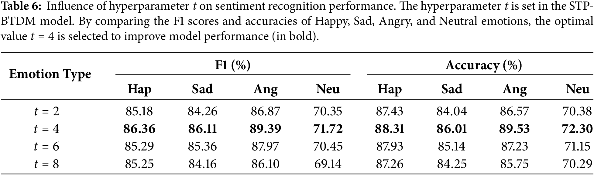
After experimenting with various hyperparameter configurations, we observed that setting t to 4 resulted in the optimal performance for the proposed method. However, when t was set to 2 or 8, the performance decreased. This occurred because setting t to 2 resulted in insufficient feature extraction accuracy, while setting t to 6 or 8 led to excessively high feature compression rates, both of which constrained the overall performance. Therefore, the configuration of t=4 will be considered in the prediction task.

6.4 Theoretical and Experimental Complexity Comparative Analysis

Here, we contrast the model complexity between the baseline model and the STP-BTDM method, as illustrated in the Table 7 below. The theoretical complexity of the model, as shown in the second column of the table, is defined by several key parameters: dy for the output feature length, In representing the input mode dimension, n denoting the number of modes, r as the tensor rank, Jn indicating the dimension of the core tensor, and m for the number of segmentation blocks. The theoretical complexity of the TFN model is approximately O(dy∏n=13In), which is a multiplication order of the input modality dimensions. On the other hand, the theoretical complexities of the LMF, STP-MFM and STP-BTDM models are approximately O(dyR∑n=13In), O(dy(∑n=131tInJn)) and O(dy(∑i=1m∑n=131tIniJni)), all of which are additive orders of the input modality dimensions.

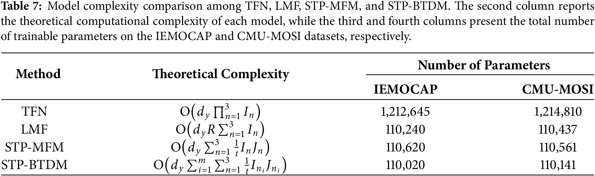
In practical operations, selecting I1=64, I2=16, I3=64, R=4, Jn=[32,8,32,2], t=4, dy=2 and m=4. In the third and fourth columns, computing the parameter count for every model across two multi-modal datasets under the above hyperparameter setting. According to the calculations presented in the table, the parameters for STP-MFM and STP-BTDM are approximately 1.1×105, while the parameters of TFN are approximately 1.2×106. Thus, the number of parameters in TFN is almost 11 times greater than that of STP-BTDM (1.2×106 vs. 1.1×105). The proposed STP-BTDM method demonstrates superior performance compared to LMF within a similar parameter range. The parameter count in the experiment also validates the theoretical complexity mentioned above. It should be noted that the parameter count listed in the table includes parameters from both the multi-modal information fusion stage and the subnet.

For the added baselines, MulT and MISA, their parameter counts are comparable to or larger than that of STP-BTDM. MulT employs multi-head cross-modal attention modules with approximately 2.8×106 parameters on CMU-MOSI, while MISA uses additional disentanglement networks and adversarial training components, resulting in roughly 3.5×106 parameters. Both are significantly more expensive than STP-BTDM (1.1×105), which achieves competitive performance with a much more compact structure, further validating the efficiency of our proposed method.

Therefore, by employing the semi-tensor product, the requirement for consistent dimensions in the multiplication of matrices is eliminated, enabling information representation in a more concise structure with reduced memory usage. More significantly, the proposed STP-BTDM framework leverages block-to-block operations through its block-term decomposition to maintain the time and space information of multiple modalities, thereby better representing the intra-modality correlation.

6.5 Analyzing Multi-Modal Fusion Examples in Emotion Analysis Tasks

In the context of tasks concerning emotion analysis, the multi-modal information fusion example analysis is illustrated by Table 8. It showcases the performance of four methods: TFN, LMF, STP-MFM and STP-BTDM in integrating multi-modal data from the CMU-MOSI dataset. Each instance is characterized by textual, auditory and visual behaviors. The predicted and true values of emotions range between strong negative (−3) and strong positive (3). While the text provides specific content for all three modalities, brief descriptions are given for visual and auditory inputs. Model performance is compared by contrasting the predicted values, true values and the absolute error across different models.

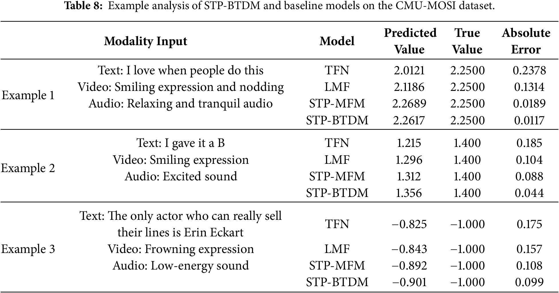
In example 1, where the true value is set at 2.2500, the predicted values for TFN, LMF, STP-MFM and STP-BTDM are 2.0121, 2.1186, 2.2689 and 2.2617, with respective absolute errors of 0.2378, 0.1314, 0.0189 and 0.0117. It is evident that the visual, auditory and textual modalities provide crucial information for expressing positive emotions and effectively demonstrate the complementarity between modalities.

Moving on to example 2, the textual word is ambiguous as the model does not know what “B” is apart from a token. However, based on the excited tone in the audio, the prediction is of a positive emotion and the smiling expression in the video also predicts a positive emotion. Thus, the audio and video modalities provide complementary evidence, resulting in the final prediction of a positive emotion, with the true value set at 1.400. The predicted values for TFN, LMF, STP-MFM and STP-BTDM are 1.215, 1.296, 1.312 and 1.356, with respective absolute errors of 0.185, 1.104, 0.088 and 0.044. All models appropriately identify this three-modal interaction.

Example 3 is intriguing because it demonstrates an interaction where the text predicts a positive sentiment based on the words, but the video shows a frowning expression, predicting a negative sentiment. Additionally, the audio has low energy, predicting a strongly negative sentiment. Therefore, the model’s final prediction almost reaches a weakly negative sentiment through strong negative visual and acoustic behaviors. The true value is set to −1.000 and the predicted values for TFN, LMF, STP-MFM and STP-BTDM are −0.825, −0.843, −0.892 and −0.901, with their absolute errors being 0.175, 0.157, 0.108 and 0.099, respectively. This example illustrates the impact of the audio modality on the model’s predictions and highlights the importance of modal complementarity.

By examining the predictions of three examples across several models, as depicted in the table, STP-BTDM outputs result closest to the actual scenarios with the smallest errors. Therefore, the approach proposed in this chapter can more effectively integrate complementary information from various modalities, thereby enhancing fusion performance.

6.6 Ablation Study on Core Components

To disentangle the contributions of each key component in STP-BTDM, we conduct a comprehensive ablation study on the CMU-MOSI dataset. We design four variants by removing or replacing individual components:

•   w/o STP: We replace the semi-tensor product with standard matrix multiplication, i.e., using ordinary Tucker decomposition instead of STP-Tucker, while retaining the block-diagonal core tensor structure.

•   w/o BTD: We remove the block-term decomposition by using a full (dense) core tensor with no block-diagonal constraint, while keeping the semi-tensor product.

•   w/o STP & BTD: We use standard Tucker decomposition without either STP or BTD, serving as the most basic baseline.

•   w/o Multilinear: We replace the multilinear pooling with simple feature concatenation of the three modalities (x1,x2,x3) followed by a fully connected layer to obtain the final prediction, while keeping the same overall network architecture.

All variants are evaluated with the same experimental setup (five runs, fixed random seeds, identical training configurations) as the full STP-BTDM. The results are summarized in Table 9.

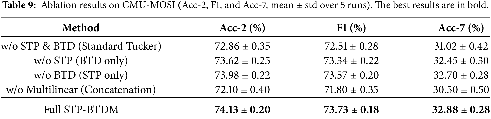
From Table 9, we observe that the removal of either STP or BTD leads to a clear performance drop, confirming that both components contribute positively to the final accuracy. Among them, BTD appears to have a slightly larger impact (dropping from 74.13% to 73.62% when STP is removed, and to 73.98% when BTD is removed, compared with the full model). The variant without both STP and BTD performs substantially worse, indicating that the combination of these two techniques is crucial for achieving competitive results. Furthermore, replacing multilinear pooling with simple concatenation causes the largest performance degradation (Acc-2 drops by about 2%), demonstrating the importance of modeling high-order interactions among modalities. Overall, the ablation study confirms that all components in STP-BTDM are effective and complementary, and the full model achieves the best performance by leveraging their synergistic advantages.

7  Related Conclusions

In this research, we introduce the Semi-Tensor Product-based Block Term Decomposition of Multilinear Pooling (STP-BTDM) method. By adopting block term decomposition based on a semi-tensor product, this method obtains a globally sparse and locally dense weight tensor, better representing the intra-modality correlation and inter-modality sparse multilinear interactions. The method uses sparse and trainable block-diagonal kernel tensors for multi-modal fusion, allowing each mode to be controlled by a block of the block-diagonal kernel independently during the training process. Moreover, in multi-modal fusion, capturing and learning different interactions of different aspects require a large global tensor, which becomes very difficult. Instead, the complexity of the block-diagonal tensor in this method lies between dense tensor and diagonal tensor and it is simple and expressive. The proposed method’s effectiveness in sentiment analysis tasks is confirmed through validation on the CMU-MOSI and IEMOCAP datasets. Experimental results show that this method outperforms three tensor-based benchmark models (TFN, LMF, and STP-MFM) and remains competitive with two recent state-of-the-art approaches, MulT and MISA, while using significantly fewer parameters (approximately 1.1×105, about 1/11 of TFN). Statistical significance testing based on five independent runs confirms that the observed improvements are reliable. The method particularly excels in fine-grained 7-class sentiment classification on CMU-MOSI, achieving the highest Acc-7 (32.88%) among all compared methods.

Acknowledgement: None.

Funding Statement: The authors received no specific funding for this study.

Author Contributions: The authors confirm contribution to the paper as follows: Conceptualization, Fen Liu; methodology, Fen Liu; software, Fen Liu; validation, Fen Liu; formal analysis, Fen Liu; investigation, Fen Liu; resources, Fen Liu; data curation, Jinghua Zhang; writing—original draft preparation, Fen Liu; writing—review and editing, Fen Liu; visualization, Weijie Tan. All authors reviewed and approved the final version of the manuscript.

Availability of Data and Materials: This study utilizes two publicly available benchmark datasets: CMU-MOSI and IEMOCAP. The CMU-MOSI dataset can be accessed at https://github.com/CMU-MultiComp-Lab/CMU-MultimodalSDK. The IEMOCAP dataset is available upon request from the USC Signal Analysis and Interpretation Laboratory (SAIL) at https://sail.usc.edu/iemocap/. The implementation code of our proposed method is available from the corresponding author upon reasonable request.

Ethics Approval: This study utilizes two publicly available benchmark datasets, CMU-MOSI and IEMOCAP, both of which contain human-subject data (including video, audio, and facial expressions) that were collected and de-identified by the original dataset creators with appropriate ethical approvals and informed consent. Our study involves only algorithmic optimization and analysis of these pre-existing, publicly available datasets. Therefore, additional ethics approval and consent to participate are not applicable.

Conflicts of Interest: The authors declare no conflicts of interest.

References

1. Daizhan C, Hongsheng Q. Semitensor product of matrices. Beijing, China: Science Press; 2007. [Google Scholar]

2. Wang M, Chen J, Zhang X, Huang Z, Rahardja S. Multi-modal speech enhancement with bone-conducted speech in time domain. Appl Acoust. 2022;200(10):109058. doi:10.1016/j.apacoust.2022.109058. [Google Scholar] [CrossRef]

3. Wang M, Chen J, Zhang XL, Rahardja S. End-to-end multi-modal speech recognition on an air and bone conducted speech corpus. IEEE/ACM Trans Audio Speech Lang Process. 2022;31:513–24. doi:10.1109/taslp.2022.3224305. [Google Scholar] [CrossRef]

4. Liu F, Chen JF, Tan WJ, Cai C. A multi-modal fusion method based on higher-order orthogonal iteration decomposition. Entropy. 2021;23(10):1349. doi:10.3390/e23101349. [Google Scholar] [CrossRef]

5. Zadeh A, Chen M, Poria S, Cambria E, Morency LP. Tensor fusion network for multimodal sentiment analysis. In: Proceedings of the 2017 Conference on Empirical Methods in Natural Language Processing; 2017 Sep 7–11; Copenhagen, Denmark. Santa Clara, CA, USA: ACL, SIGDAT; 2017. p. 1103–14. [Google Scholar]

6. Abdu SA, Yousef AH, Salem A. Multimodal video sentiment analysis using deep learning approaches, a survey. Inf Fusion. 2021;76(3):204–26. doi:10.1016/j.inffus.2021.06.003. [Google Scholar] [CrossRef]

7. Poria S, Cambria E, Bajpai R, Hussain A. A review of affective computing: from unimodal analysis to multimodal fusion. Inf Fusion. 2017;37:98–125. [Google Scholar]

8. Cheng DZ, Qi HS, Zhao Y. An introduction to semi-tensor product of matrices and its applications. 2012 [cited 2026 Jan 1]. Available from: http://www-personal.umich.edu/. [Google Scholar]

9. Cheng D, Qi H. Semi-tensor product of matrices—theory and applications. Beijing, China: Science Press; 2007. [Google Scholar]

10. Cheng D, Qi H, Li Z. Analysis and control of boolean networks: a semi-tensor product approach. New York, NY, USA: Springer Science & Business Media; 2010. [Google Scholar]

11. Fen L, Jianfeng C, Kemeng L, Jisheng B, Weijie T, Chang C, et al. STP-MFM: semi-tensor product-based multi-modal factorized multilinear pooling for information fusion in sentiment analysis. Digit Signal Process. 2024;145:104265. [Google Scholar]

12. Picard RW. Affective computing for HCI. In: Proceedings of the HCI International (The 8th International Conference on Human-Computer Interaction) on Human-Computer Interaction: Ergonomics and User Interfaces; 1999 Aug 22–27; Munich, Germany. p. 829–33. [Google Scholar]

13. Duc B, Bigün ES, Bigün J, Maître G, Fischer S. Fusion of audio and video information for multi modal person authentication. Pattern Recognit Lett. 1997;18(9):835–43. doi:10.1016/s0167-8655(97)00071-8. [Google Scholar] [CrossRef]

14. Ross AA, Nandakumar K, Jain AK. Handbook of multibiometrics. Vol. 6. New York, NY, USA: Springer Science & Business Media; 2006. [Google Scholar]

15. D’mello SK, Kory J. A review and meta-analysis of multimodal affect detection systems. ACM Comput Surv. 2015;47(3):43:1–36. doi:10.1145/2682899. [Google Scholar] [CrossRef]

16. Wang X, Chen X, Cao C. Human emotion recognition by optimally fusing facial expression and speech feature. Signal Process Image Commun. 2020;84(10):115831. doi:10.1016/j.image.2020.115831. [Google Scholar] [CrossRef]

17. Kansizoglou I, Bampis L, Gasteratos A. An active learning paradigm for online audio-visual emotion recognition. IEEE Trans Affect Comput. 2019;13(2):756–68. [Google Scholar]

18. Nguyen D, Nguyen K, Sridharan S, Dean D, Fookes C. Deep spatio-temporal feature fusion with compact bilinear pooling for multimodal emotion recognition. Comput Vis Image Underst. 2018;174(5):33–42. doi:10.1016/j.cviu.2018.06.005. [Google Scholar] [CrossRef]

19. Gkoumas QLD, Lioma G, Yu YJ, Song DW. What makes the difference? An empirical comparison of fusion strategies for multimodal language analysis. Inf Fusion. 2021;66(6):184–97. doi:10.1016/j.inffus.2020.09.005. [Google Scholar] [CrossRef]

20. Han Z, Wang J. Feature fusion algorithm for multimodal emotion recognition from speech and facial expression signal. In: MATEC Web of Conferences. Vol. 61. Les Ulis, France: EDP Sciences; 2016. [Google Scholar]

21. Kolda TG, Bader BW. Tensor decompositions and applications. SIAM Rev. 2009;51(3):455–500. doi:10.1137/07070111X. [Google Scholar] [CrossRef]

22. Liu Z, Shen Y, Lakshminarasimhan VB, Liang PP, Zadeh A, Morency LP. Efficient low-rank multimodal fusion with modality-specific factors. In: Proceedings of the 56th Annual Meeting of the Association for Computational Linguistics; 2018 Jul 15–20; Melbourne, Australia. p. 2247–56. [Google Scholar]

23. Zhao Z, Wang Y, Shen G, Xu Y, Zhang J. TDFNet: transformer-based deep-scale fusion network for multimodal emotion recognition. IEEE/ACM Trans Audio Speech Lang Process. 2023;31:3771–82. doi:10.1109/TASLP.2023.3316458. [Google Scholar] [CrossRef]

24. Sun Z, Zhang H, Bai J, Liu M, Hu Z. A discriminatively deep fusion approach with improved conditional GAN (im-GGAN) for facial expression recognition. Pattern Recognit. 2023;135:109157. doi:10.1016/j.patcog.2022.109157. [Google Scholar] [CrossRef]

25. Peng H, Gu X, Li J, Wang Z, Xu H. Text-centric multimodal contrastive learning for sentiment analysis. Electronics. 2024;13(6):1149. doi:10.3390/electronics13061149. [Google Scholar] [CrossRef]

26. Liu W, Qiu JL, Zheng WL, Lu BL. Comparing recognition performance and robustness of multimodal deep learning models for multimodal emotion recognition. IEEE Trans Cogn Dev Syst. 2021;14(2):715–29. doi:10.1109/tcds.2021.3071170. [Google Scholar] [CrossRef]

27. Schoneveld L, Othmani A, Abdelkawy H. Leveraging recent advances in deep learning for audio-visual emotion recognition. Pattern Recognit Lett. 2021;146:1–7. [Google Scholar]

28. Zhou H, Du J, Zhang Y, Wang Q, Liu QF, Lee CH. Information fusion in attention networks using adaptive and multi-level factorized bilinear pooling for audio-visual emotion recognition. IEEE/ACM Trans Audio Speech Lang Process. 2021;29:2617–29. doi:10.1109/TASLP.2021.3094952. [Google Scholar] [CrossRef]

29. Lian Z, Liu B, Tao J. SMIN: semi-supervised multi-modal interaction network for conversational emotion recognition. IEEE Trans Affect Comput. 2023;14(3):2415–29. doi:10.1109/TAFFC.2022.3141237. [Google Scholar] [CrossRef]

30. Baltrusaitis T, Ahuja C, Morency LP. Multimodal machine learning: a survey and taxonomy. IEEE Trans Pattern Anal Mach Intell. 2019;41(2):423–43. [Google Scholar]

31. Cheng D. Semi-tensor product of matrices and its application to Morgens problem. Sci China Ser Inf Sci. 2001;44(3):195–212. doi:10.1007/bf02714570. [Google Scholar] [CrossRef]

32. Cheng DZ, Qi HS. A linear representation of dynamics of boolean networks. IEEE Trans Autom Control. 2010;55(10):2251–8. doi:10.1109/tac.2010.2043294. [Google Scholar] [CrossRef]

33. Zadeh A, Zellers R, Pincus E, Morency LP. Mosi: multimodal corpus of sentiment intensity and subjectivity analysis in online opinion videos. arXiv:1606.06259. 2016. [Google Scholar]

34. Busso C, Bulut M, CCea L. IEMOCAP: interactive emotional dyadic motion capture database. Lang Resour Eval. 2008;42:335–59. [Google Scholar]

35. Yuan J, Liberman M. Speaker identification on the SCOTUS corpus. J Acoust Soc Am. 2008;123(5):3878. doi:10.1121/1.2935783. [Google Scholar] [CrossRef]

36. Pennington J, Socher R, Manning C. Glove: global vectors for word representation. In: Proceedings of the 2014 Conference on Empirical Methods in Natural Language Processing (EMNLP); 2014 Oct 25–29; Doha, Qatar. p. 1532–43. [Google Scholar]

37. Degottex G, Kane J, Tea D. COVAREP—a collaborative voice analysis repository for speech technologies. In: Proceedings of the IEEE International Conference on Acoustics, Speech and Signal Processing; 2014 May 4–9; Florence, Italy. p. 960–4. [Google Scholar]

38. Ekman P. An argument for basic emotions. Cogn Emot. 1992;6(3–4):169–200. doi:10.1080/02699939208411068. [Google Scholar] [CrossRef]

39. Ekman P, Friesen WV, Ancoli S. Facial signs of emotional experience. J Pers Soc Psychol. 1980;39(6):1125–34. doi:10.1037/h0077722. [Google Scholar] [CrossRef]

40. Tsai YH, Bai S, Pu Liang P, Kolter JZ, Morency LP, Salakhutdinov R. Multimodal transformer for unaligned multimodal language sequences. In: Proceedings of the 56th Annual Meeting of the Association for Computational Linguistics; 2018 Jul 15–20; Melbourne, Australia. p. 6558–69. [Google Scholar]

41. Hazarika D, Zimmermann R, Poria S. Misa: modality-invariant and-specific representations for multimodal sentiment analysis. In: Proceedings of the 28th ACM International Conference on Multimedia; 2020 Oct 12–16; Seattle, WA, USA. p. 1122–31. [Google Scholar]