An Isogeometric Cloth Simulation Based on Fast Projection Method

1  Introduction

Cloth simulation has many practical applications, such as computer-aided garment design, character animation, and electronic e-commerce. Terzopoulos et al. [1] were among the first to develop a physical model for use in the simulation of cloth. Breen et al. [2–4] developed a spring-based model, and their initial motivation was to accurately represent complex fabric behaviors using nonlinear springs. Provot [5] modeled cloth by employing linear springs characterized by low stiffness and he achieved acceptable results with high efficiency. Eischen et al. [6] modeled cloth using finite-element shell theory. Baraff et al. [7] proposed to employ implicit time integration to increase the time step, while the Newton iteration was suggested to be halted at the first step to achieve high efficiency. Choi et al. [8] proposed an immediate buckling model to ensure that the Jacobi matrix in the implicit method was definite. Bridson et al. employed a velocity Verlet algorithm [9] to increase the time increment. In addition to the cloth model, the collision response was also largely improved. Baraff et al. [7] simulated collision as a velocity constraint and Bridson et al. [10] proposed a decoupled bullet-proof collision scheme.

The garment industry is now beginning to use virtual simulation for prototyping [11,12]. However, as reported in [13], there are still many challenges in the application of virtual simulation. One of the challenges is to develop a high-efficiency continuum approach. The continuum approach has many advantages over the spring-based approach. For example, the material properties of the continuum approach are independent of the topology of the grid. Another attraction of the continuum approach is that many studies of material and geometric nonlinearity have been conducted in this field. However, conventional finite-element shell theory has low efficiency due to two reasons: (1) it needs more degrees of freedom for the same grid, and (2) the collision response is more complex.

Another challenge of cloth simulation is how to efficiently enforce realistic strain on cloth. One of the characteristics of fabric is that the bending stiffness is far lower than the in-plane stiffness. A consequence of this property is that in-plane deformation of practical cloth in most cases is negligible if compared to the out-of-plane deformation. However, using high physical in-plane stiffness introduces significant difficulty in simulation. For explicit methods, higher in-plane stiffness requires smaller time increments. In Barraf et al. [7] semi-implicit method, the frictional damping is proportional to the in-plane stiffness. Thus, to reduce the computational burden, in many practical cloth simulations, the value of the in-plane stiffness is artificially reduced to enable the simulation of more complex problems in reasonable time. However, this approach can introduce unrealistic overstretching of the cloth.

To overcome this undesired side effect, Provot [5] proposed an explicit method of strain limiting that restores the over-stretched springs by adjusting the particle position directly. Because adjusting the position of one spring may result in over-stretching of another spring, an iteration is required. Both Jacobi and Gauss-Seidel iterations [10] are utilized, but neither one can guarantee convergence. Implicit methods of strain limiting have also been proposed [4,14]. These approaches are mainly based on the constrained Lagrange method and consider in-plane strain as a constraint condition. Goldenthal et al. [15] proposed a fast projection method that can solve the constrained Lagrange problem much more efficiently. The implicit method requires solving a linear system for each iteration, but it can converge very quickly. The fast projection method in [15] constrains the spring length of a weft and warp aligned quadrilateral grid, but this kind of grid is difficult to obtain for practical garments. To obtain a grid-independent strain-limiting scheme, one must resort to a continuum model. Studies of continuum-based strain limiting are limited at present. Thomaszewski et al. [16] proposed explicit strain limiting for triangular elements.

Isogeometric analysis has been proposed to bridge computer-aided design (CAD) and analysis seamlessly [17]. The IGA owns the salient features such as higher-order continuity and exact geometry preservation etc., which provides an effective solution for problems that conventional finite element methods are not proper qualified to solve [18–20], thus it has received much attention in many fields. For cloth simulation, a systematic method is proposed by the authors [21]. This method uses the rotational-free Kirchhoff-Love shell model [22,23], wherein CAD geometry is directly utilized in analysis. Recent developments in cloth-like simulation involve large deformation shells or membrane modeling [24–26]. The present work proposes a continuum version of a strain-limiting scheme by applying the fast projection method, such that the shell model for cloth simulation can be solved quickly with an acceptable resultant shape. Another advantage of this model is that it performs the simulation directly on the NURBS surface, which is widely implemented in CAD software. This property ensures the high fidelity of the simulated cloth and provides convenience of interactive design in three-dimensional (3D) space.

The rest of this paper is organized as follows. Section 2 briefly reviews the rotation-free Kirchhoff-Love Shell on a NURBS basis. Section 3 outlines the continuum-based fast projection method for (trimmed) NURBS geometry. Finally, four example problems are solved to validate the proposed approach and their results are presented in Section 4. Conclusions are presented in Section 5.

2  NURBS Kirchhoff-Love Shell

Kirchhoff-Love shell theory assumes the following:

•   The normal to the undeformed middle surface remains straight and perpendicular to the deformed middle surface.

•   The transverse normal stress is small compared with other normal stress components and may be neglected.

•   The thickness of the shell is small compared to the other dimensions.

•   The displacements of any given point on the shell are small in comparison to the thickness.

These assumptions are a good approximation for fabrics in which the energetic contribution from transverse shear is negligibly small compared to the bending and in-plane energy. Hence, the kinetics are completely characterized by the surface strain and curvature, which are determined by the surface geometry. For numerical computation, the theory can lead to a displacement-only formulation, which does not involve rotational degrees of freedom, thus increasing the efficiency of the method. A Kirchhoff-Love shell element is not commonly used in traditional finite-element analysis because constructing a C1 continuous surface is difficult for some element topologies. However, with NURBS geometry, it is straightforward to construct surfaces of C1 or even higher-order continuity. For this and other considerations, the NURBS Kirchkoff-Love shell is utilized for cloth modeling.

In the present NURBS Kirchkoff-Love shell element, the primary unknowns are the displacements of the control points. No rotational degree-of-freedoms are introduced.

2.1 Kinematics

The NURBS formulation below follows that of Kiendl et al. [22]. We use the same set of NURBS basis functions to parameterize the reference and current configurations of the cloth surface:

X=∑I=1nNI(ξ1,ξ2)QI(1a)

x=∑I=1nNI(ξ1,ξ2)qI(1b)

Here, the QIs are the reference coordinates of control points and the qI are the current coordinates. The NIs are the basis functions of the NURBS surface. The knot parameters ξ=(ξ1,ξ2) serve as the convected coordinates whereby a fixed pair ξ represents the same material point throughout deformation. These two coordinates induce two convected surface basis vectors a1=x,ξ1anda2=x,ξ2 spanning the tangent plane at every point of the surface. A line element in the current configuration is thus represented as dx=a1dξ1+a2dξ2. In the reference configuration, the surface bases are denoted {A1,A2}, and a line element is given by dX=A1dξ1+A2dξ2. The basis vectors are illustrated in Fig. 1.

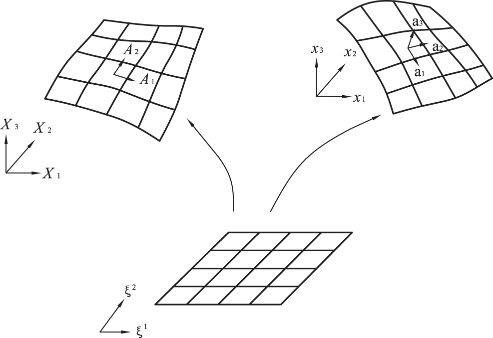
Figure 1: Illustration of shell kinematics

The unit normal a3 (in the current configuration) is

a3=a1×a2∥a1×a2∥(2)

With respect to the convected basis vectors, the surface deformation tensor C and Green-Lagrangian strain E take the forms

Cαβ=aα⋅aβ,α,β=1,2(3a)

Eαβ=12(aα⋅aβ−Aα⋅Aβ)α,β=1,2(3b)

respectively. The surface curvature tensor κ is defined by

καβ=−∂a3∂ξα⋅aβ=a3⋅∂2x∂ξα∂ξβ,α,β=1,2(4)

It is convenient to use a local ortho-normal basis to perform the element computations presented later. To this end, we introduce a pair of orthonormal bases {E¯1,E¯2} point-wise in the tangent plane spanned by {A1,A2}. With respect to the new bases, we express a line element as dX=E¯1dX¯1+E¯2dX¯2. Locally, (dX¯1,dX¯2) are related to (dξ1,dξ2) via

[dX¯1dX¯2]=[E¯1⋅A1E¯1⋅A2E¯2⋅A1E¯2⋅A2][dξ1dξ2]:=Jdξ(5)

Derivatives of a basis function N in local physical coordinates follow the chain rule:

[N,X¯1N,X¯2]=J−T[N,ξ1N,ξ2](6)

In the current configuration, the bases (a¯2, a¯2) convected from the physical basis {E¯1,E¯2} are

a¯α:=∂x∂X¯1=∑INI,X¯αqI,α=1,2(7)

With respect to the physical basis, the Green-Lagrangian strain assumes the form E¯αβ=12(a¯α⋅a¯β−δαβ). The physical components of the curvature tensor can be obtained by the transformation κ¯αβ=∂ξδ∂X¯ακδγ∂ξγ∂X¯β.

The local bases {E¯i} can be selected in many ways, but we suggest aligning the local bases with the weft and warp direction of the fibers, which are pre-defined by users.

2.2 Constitutive Law

Cloth response is typically inelastic, exhibiting anisotropic properties and a small to moderate amount of hysteresis [27–29]. Since the focus of the present work is on geometry, we simplify the constitutive description by using an isotropic elastic model. The in-plane strain of fabrics is usually small (<2%); however, since large rotation is involved, the use of finite strain is necessary. Because of the small strain range, any mechanically sound finite-strain constitutive model should reasonably describe the in-plane response. Here, we use a linear anisotropic relation [7] between the (in-plane) Piola-Kirchhoff stress S and Green-Lagrangian strain E:

SI=kIEI(8)

in which I can be replaced by “weft,” “warp,” or “shear,” and kI is a material constant.

For the bending model, we employ a nonlinear bending function [29] for curvatures in weft and warp directions,

mI={sign(κI)2B0κ0|κI|,|κI|≤κ0sign(κI)(B0|κI|+B0κ0),|κI|>κ0(9)

where I can be replaced by “weft” or “warp,” and B0 and κ0 are material constants. The bending curve is depicted in Fig. 2. The shape mimics the ascending portion of a typical fabric bending in a Kawabata test [30]. The bending moment, in general, depends on curvature change; here, the reference curvature is taken to be zero.

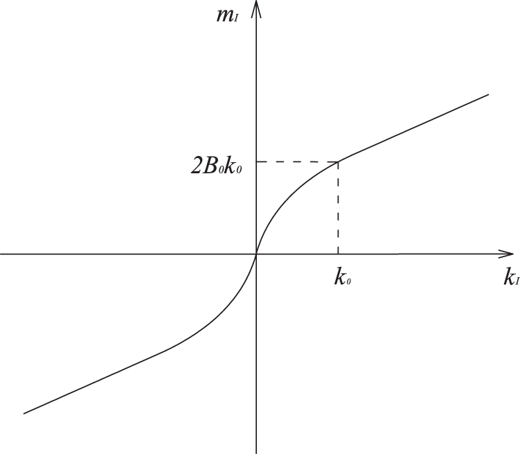
Figure 2: Moment-curvature curve in principal space

2.3 Element Equation

External forces acting on a piece of cloth normally include a body force ρb and damping force fd (per unit surface area); that is, in general, a function of the cloth velocity, and traction forces t¯ prescribed on the boundary edge. Following the textile community convention, we use the surface density ρ to describe the mass distribution; ρ=ρ0h, where ρ0 is the 3D density and h is cloth thickness. The weak form of the dynamics equilibrium equation is given by

∫ΩρδuTadA+∫Ω(hδETS+δκTm)dA=∫Ω(δuT(ρb+fd)dA+∫Γt(δuTt¯)hds(10)

In the NURBS representation, u=x−X=∑INI(qI−QI), and thus

δu=Nδq,N=[N1IN2I⋯](11)

where I is the 3 × 3 identity matrix. The variation of Green-Lagrangian strain, in Voigt form, δE=(δE11,δE22,2δE12), is derived as

δE=Bmδq,Bm=(B11m1B11m2…B22m1B22m2…2B12m12B12m2…)(12)

where

(BαβmI)T=∂Eαβ∂qI=12(NI,βaα+NI,αaβ)(13)

Similarly, from the definition of curvature, we can derive

δκ=Bbδq,Bb=(B11b1B11b2…B22b1B22b2…2B12b12B12b2…)(14)

where

(BαβbI)T=∂καβ∂qI=NI,αβa3+1j[NI,1(a2×x,αβ)+NI,2(x,αβ×a1)]−(x,αβ⋅a3)(NI,1a1+NI,2a2)(15)

In the above, j=||a1×a2|| is the area stretch, and (a1,a2) are the bases dual to (a1,a2) satisfying aα⋅aβ=δβα and aα⋅a3=0.

Substituting Eqs. (11), (12), and (14) into Eq. (10) yields the discrete dynamic equation

Mq..−fdampq.+fintq=fext(16)

where

M=∫ΩNTNρdA(17a)

fint=∫Ω(hBmTS+BbTm)dA(17b)

fext=∫ΩNTρbdA+∫ΓtNTt¯hds(17c)

fdamp=∫ΩNTfddA(17d)

For low-speed air drag, we assume that fd=−ηx., where η is a viscosity constant; in this case, fdamp=−ηρMq.:=−Dq..

2.4 Time Integration

Our strain-limiting scheme is independent of time integration. Here, we use the velocity Verlet scheme that was first applied to cloth simulation by [9]. The flow process for time integration is as follows:

1.    Predict average velocity and candidate configuration at tn+1,

{q.n+12=q.n+12q..nΔt,qn+1=qn+q.~n+12Δt(18)

2.    Compute q˙n+1,q¨n+1 from

{Mq..n+1+Cq.n+1+fint(qn+1)=fext(tn+1)q.n+1=q.n+12+Δt2q..n+1(19)

3  Continuum-Based Fast Projection Method

3.1 Constrained Lagrange Method

The fast projection method begins with the constrained Lagrange problem. For the general coordinates r=(qT,λT), the constraint Lagrange potential is given by

L(r,r˙)=12q˙TMq˙−V(q)−C(q)Tλ(20)

in which C is a set of constraint conditions that stops in-plane stretching.

The Euler-Lagrange equation is:

∂L∂r−ddt∂L∂r.=0(21)

Thus, we have,

Mq..=−∂V∂q−∂CT∂qλ(22a)

C=0(22b)

Supposing that we check the constraint condition at the end of a time step, C(qn+1=0), and use the velocity Verlet scheme for internal dynamics, we then have:

qn+1=qn+h(q.n−h2M−1∂V(qn)∂q)−h2M−1(∂C(qn+1)T∂qλn+1)(23a)

C(qn+1)=0(23b)

Now, we use the splitter:

1.    Predict candidate configuration q~n+1 by internal dynamics (without constraints)

q~n+1=qn+h(q.n−h2M−1∂V(qn)∂q)(24)

This sub-step can be replaced by any time-integration scheme.

2. Correct the candidate configuration by qn+1=q~n+1+Δq, and solve Δq from

Δq=−h2M−1∂C(qn+1)T∂qλn+1(25a)

C(qn+1)=0(25b)

Eqs. (25a) and (25b) are equivalent to δW=0, where

W=12h2ΔqTMΔq+C(qn+1)Tλn+1(26)

The second term of W projects q into the constraint manifold, while the first term minimizes the change of kinematic energy in this projecting process. All together, q will be projected to the “closest” point on the constraint manifold.

Linearizing Eqs. (25a) and (25b) by the Newton method, we have the following flow process:

Δq[0]=0, λ[0]=0, for j = 0, 1, 2,…, do

1.    Solve Δq and dλ from

[I+h2M−1∂C[j]Tλ[j]∂q∂qh2M−1∂C[j]T∂q∂C[j]∂q0][dqdλ]=[−Δq[j]−h2M−1∂C[j]T∂qλj−C[j]](27)

2.    Correct q and λ by

Δq[j+1]=Δq[j]+dq,λ[j+1]=λ[j]+dλ(28)

The iteration exits when the C is smaller than a given tolerance. We note here that we must solve a (3n+m)-dimensional asymmetric linear system for each iteration.

3.2 Fast Projection Scheme

We note that Eq. (25a) keeps the property of “closest” and Eq. (25b) keeps the constraint conditions. In the actual problem, we have a high requirement on constraint conditions but a low requirement on the property of “closest.” Goldenthal et al. [15] suggested solving Eq. (25a) using the Euler method while solving Eq. (25b) using the Newton method. We expand C by a Taylor series at q[j] and ignore the quadratic and higher-order terms

C[j+1]=C[j]+∂C∂qdq(29)

Substituting Eq. (29) into Eq. (25a) yields

dq=−h2M−1∂C[j]T∂qdλ(30)

Eq. (25b) is still linearized by the Newton method

∂C[j]∂qdq=−C[j](31)

Substituting Eq. (30) into Eq. (31) yields the basic equation of the fast projection method

h2∂C[j]∂qM−1∂C[j]T∂qdλ=Cj(32)

The iterative fast projection process flow is as follows:

Δq[0]=0, for j = 0, 1, 2,…

1.    Solve dλ from

h2∂C[j]∂qM−1∂C[j]T∂qdλ=Cj(33)

2.    Correct q by

Δq[j+1]=Δq[j]−h2M−1∂C[j]T∂qdλ(34)

The iteration exits when the C is smaller than the given tolerance. The advantage of the fast projection method is that: (1) we only need to solve an m-dimensional S.P.D. linear system for each iteration, and (2) it converges faster.

3.3 Spring-Based Fast Projection

For the spring-mass method, the length of each spring is a constraint, C=[C1,C2,…], and

Ci=li/Li−1(35)

in which li and Li are the current and referent lengths of the ith spring, respectively. For triangular mesh, because the total number of springs is approximately 3 times the total number of nodes, the deformation of the entire mesh is locked and even curvature is not allowed. Thus, quad-dominated mesh is required.

3.4 Continuum-Based Fast Projection

For the continuum-based approach, the first task is to select sampling points. We tried to select the Gaussian points as sampling points, but that does not work well. Because the number of cells are close to the number of control points, and if there are three or more constraint conditions on each cell, the model will be locked. Thus, 2×2 or more Gaussian points are not allowed. We then tried one Gauss point and the average strain, but both schemes display the hourglass problem. By adding a certain term to the averaged strain scheme, we might have been able to eliminate the hourglass problem, but instead we decided to try a different approach. We selected vertices of a knot mesh as sampling points, as shown in Fig. 3. For trimmed NURBS, we constrain the intersection points between the trimming curve and knot mesh as well. The benefit of this scheme is that it does not have locking or hourglass problems, and it can minimize the bandwidth of the coefficient matrix ∂C[j]∂qM−1∂C[j]T∂q.

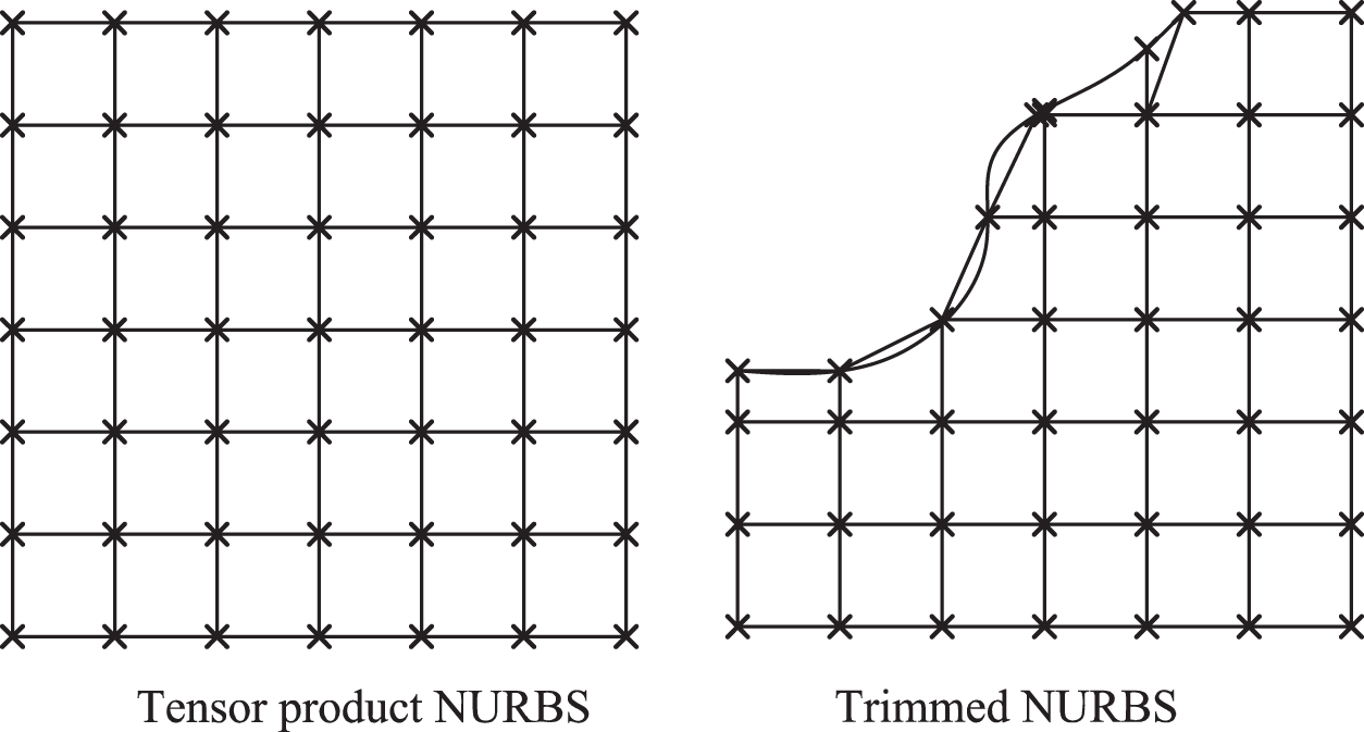
Figure 3: Constraint points

The constraint condition C is expressed as CT=[C1T,C2T…], in which Ci is a constraint on one sampling point. For each sampling point, we can set, at most, two constraints. Considering that the shear stiffness of fabric is far lower than the stretch stiffness in weft and warp directions, we constrain the strain in weft and wart directions, given by:

Ci=[Eweft,Ewarp]T(36)

in which Eweft and Ewarp are the strains in the weft and warp directions of the fabric, respectively. Noting that the local bases E¯1 and E¯2 are defined as any pair of orthogonal vectors in the tangent plane spanned by A1 and A2, a simple way to compute Eweft and Ewarp is to set E¯1 and E¯2 aligned with the weft and warp directions.

3.5 Stress Reconstruction

The constraint energy term λ⋅C, in essence, is the nodal integration form of strain energy. Thus, the stress S^ should include two terms: the stress from strain S(E) and that from constraint force. The stress on grid point i after fast projection is given by

S^i=Si(Ei)+λi/ai(37)

where ai is the nodal area.

However, we found a checkerboard pattern in the values of λ. This is mainly due to the lack of domain integration. Introducing the integration version of constraint energy may resolve the problem, but we believe that is to costly as the bandwidth will be heavily enlarged. Therefore, we introduced a simple way to reconstruct the stress: by an interpolation, which makes it easy to obtain the stress on Gaussian points. Then, by an extrapolation from Gaussian points, we can obtain the nodal stress without a checkerboard problem.

4  Examples

4.1 Corner Kidnapped Cloth

A piece of cloth in the x-y plane is subject to constraints at two corners and will swing under gravity in the z direction. The cloth is represented by a second-order NURBS patch with 100 control points. The bending parameters are B0=3.3×10−3N⋅m, κ0=30m−1. The mass density is ρ=0.117kg/m2 and the damping constant is η=0.351kg/(m2⋅s). Fabric thickness is h=0.001177m. For the in-plane model, we assume k=kweft=kwarp=2.5kshear and test three cases: (a) k/ρ=100, strain limit = 0.01; (b) k/ρ=5000 without strain limiting; and (c) k/ρ=100 without strain limiting.

The simulation results of different Young’s moduli at t=0.6s (the cloth passes the vertical plane for the first time near this time) are shown in Fig. 4. The simulation time and strain summary are shown in Table 1. It is observed that case (c) has obvious unrealistic stretching. The results of cases (a) and (b) are close, but the time increment of case (a) is much smaller than that of case (b). Because there is no contact involved, the time savings of a large time increment is not very obvious; however, strain limiting still obtains a speedup of 2.5 times.

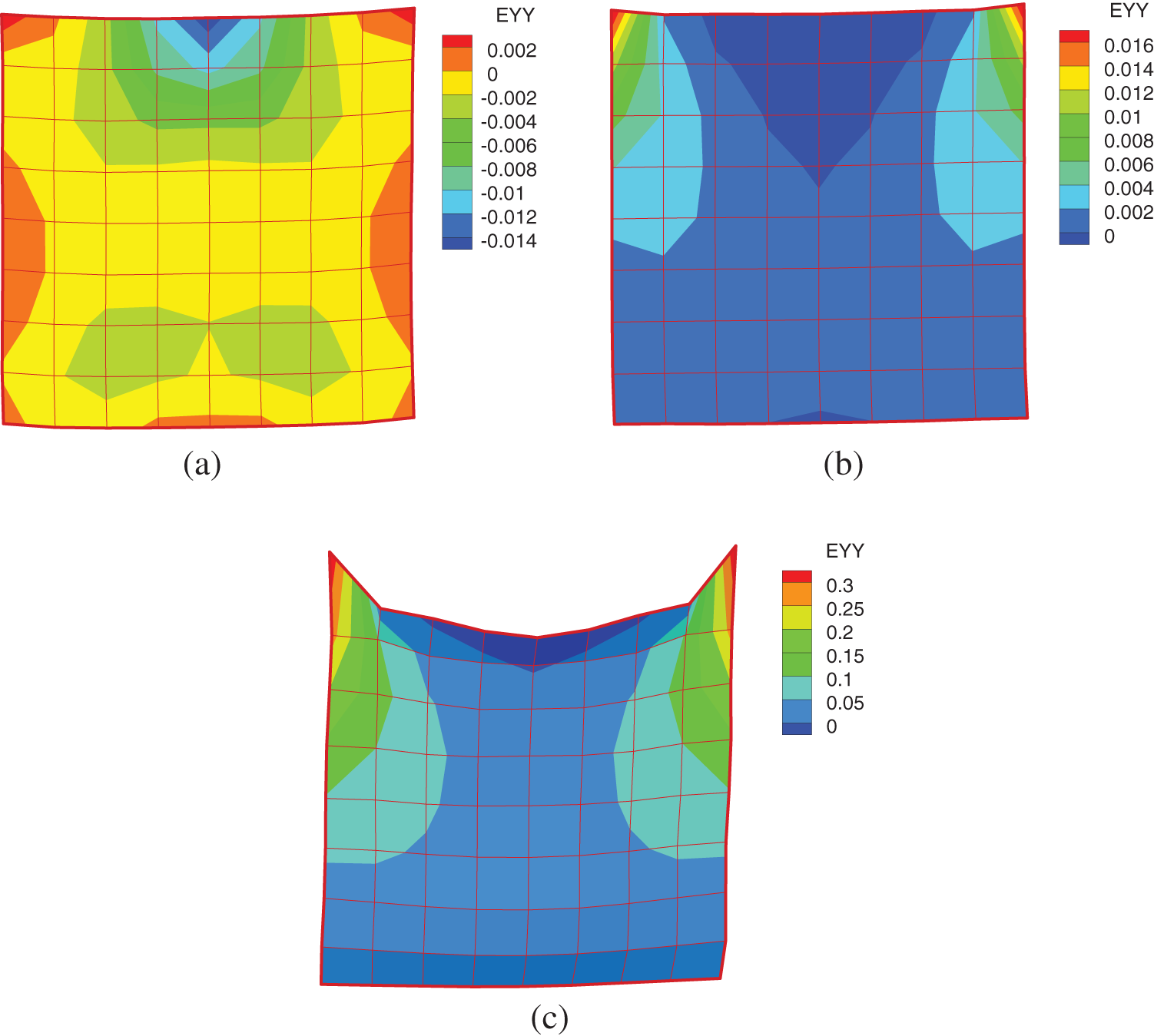
Figure 4: Corner kidnapped cloth at t =  0.6 for cases (a)–(c)

4.2 Draping of Soft Armor

The draping of a soft armor was simulated in this example. The armor is represented by a second-order NURBS patch with 1,616 control points. The initial configuration is obtained by virtual try-on simulation and is shown in Fig. 5. The bending parameters are B0=1×10−4N⋅m, κ0=30m−1. The mass density is ρ=0.1177kg/m2 and the damping constant is η=0.353kg/(m2⋅s). Fabric thickness is h=0.001177m. The friction coefficient is assumed to be μ=0.2. For the in-plane model, we assume k=kweft=kwarp=2.5kshear and create three cases: (a) k/ρ=50, strain limit = 0.01; (b) k/ρ=5000 without strain limiting; and (c) k/ρ=50 without strain limiting.

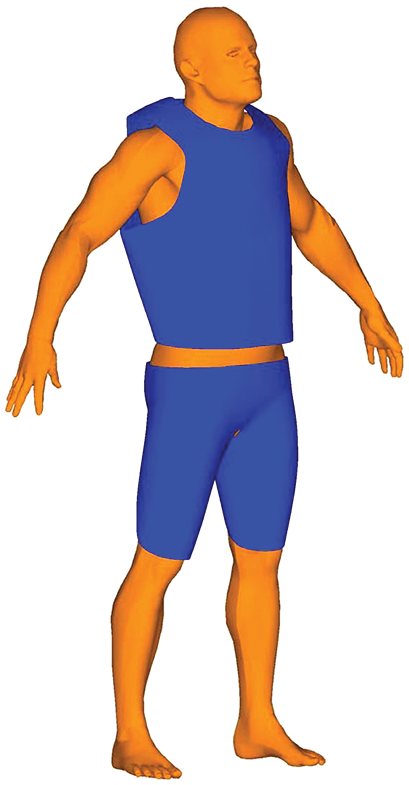
Figure 5: Initial configuration of soft armor

To more clearly show the results, the simulation results of upper- and lower-body armor at t=0.5s are shown in Figs. 6 and 7, respectively. The simulation time and strain summary are shown in Table 2. For the upper-body armor, case (c) obtains an unacceptable shape, while for lower-body armor all three schemes obtain an acceptable shape. By checking the maximum and average strain, it is found that both cases (a) and (b) obtain a low level of strain, but the time cost of case (b) is much greater than case (a). This demonstrates that the strain-limiting method can reduce strain level by reducing extra CPU cost rather than by pure high stiffness.

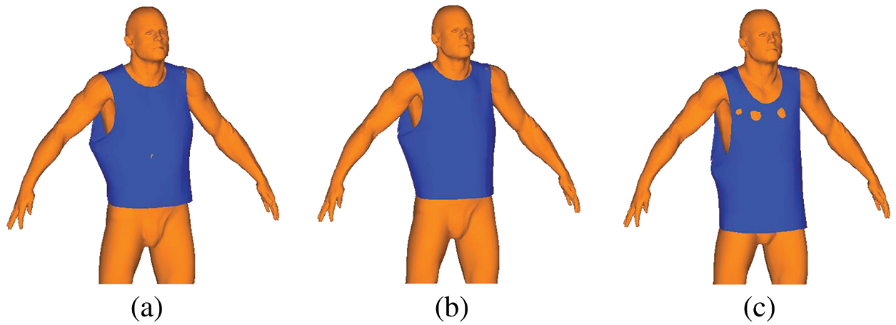
Figure 6: Upper-body armor after draping simulation for cases (a)–(c)

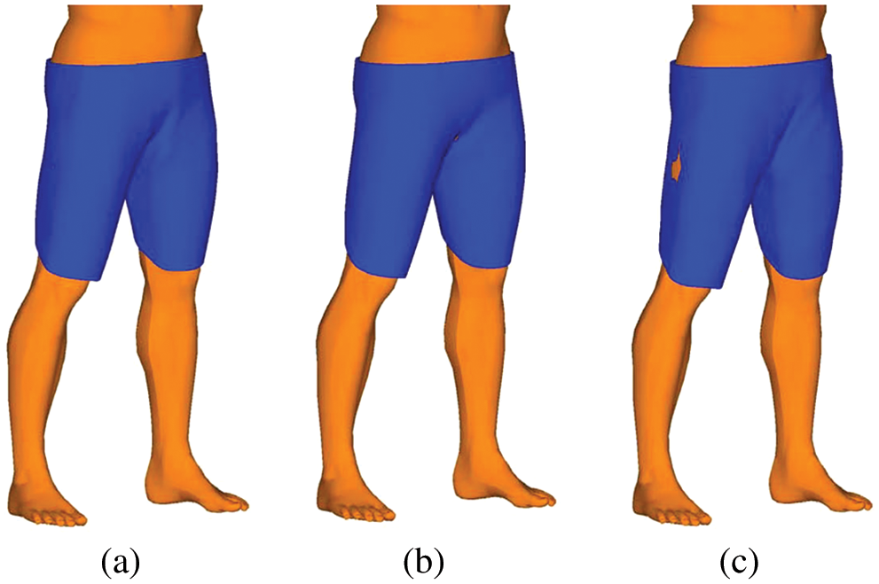
Figure 7: Lower-body armor after draping simulation for cases (a)–(c)

4.3 Draping of a Skirt

This example simulates the draping process of a skirt. The initial configuration of the skirt is obtained by a try-on simulation and is shown in Fig. 8. The entire model contains 960 control points. The woman’s body is represented by a discrete mesh of 17,068 cells. The bending parameters are B0=1.0×10−5N⋅m and κ0=30m−1. The mass density is ρ=0.118kg/m2 and the damping constant is η=0.354kg/(m2⋅s). The fabric thickness is h=0.001177m. A friction coefficient μ=0.8 is assumed. For the in-plane model, we assume k=kweft=kwarp=2.5kshear and create three cases: (a) k/ρ=50, strain limit = 0.01; (b) k/ρ=3000 without strain limiting; and (c) k/ρ=50 without strain limiting.

Figure 8: Initial configuration of skirt

The garment shape at t=0.8s, when the vibrations are mostly damped out, is shown in Fig. 9. The simulation time and strain summary are shown in Table 3. It is observed that low stiffness without strain limiting obtains an unacceptable shape. When E/ρ=3000 and strain limiting is turned off, the simulation shape looks better, but local over-stretching still occurs. We did not try a higher stiffness because it takes too much time. However, by using the proposed strain-limiting scheme, both the simulation shape and strain values satisfied requirements while keeping the time cost very low.

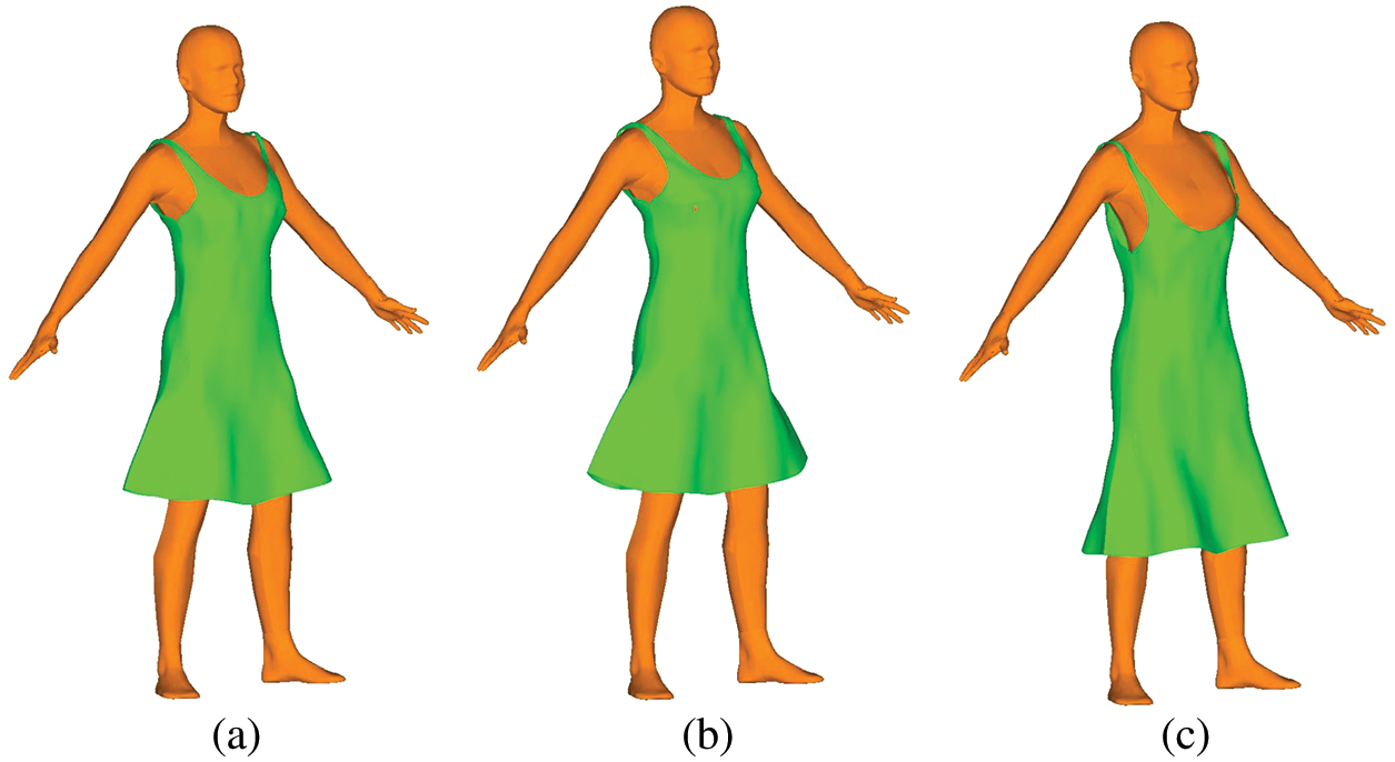
Figure 9: Skirt after draping simulation for cases (a)–(c)

4.4 Patch Test

Finally, we conducted a standard patch test to check the stress obtained from the fast projection method. A 1 m-by−1 m square was fixed on the top edge and we applied 1 N/m of uniform force on the bottom edge. As the problem itself is based on dynamic analysis, we modeled the static patch test by applying a large damping factor and waiting until the vibration was damped out. Fig. 10 shows the static stress obtained from analysis with or without the fast projection method. It is observed that for both cases the stresses are close to 1 Pa, which means that the fast projection method cannot only eliminate unrealistic strain, but can also provide a reliable stress field.

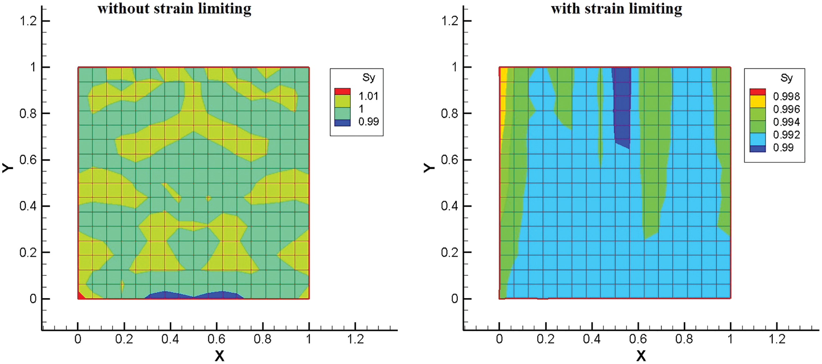
Figure 10: Patch test stress

5  Conclusions

In this work, a rotational-free Kirchhoff-Love shell-based isogeometric analysis was outlined for cloth simulation. To overcome the numerical burden caused by high in-plane stiffness, a continuum version of the fast projection method was applied. The highlights of this work are the following:

•   Compared with spring-based models, the constraint directions of strain limiting are independent of grid lines. This implies that the fast projection method can be applied to a grid with arbitrary topology.

•   Examples show that the present scheme can eliminate unrealistic over-stretching efficiently, while the stress field remains reliable.

•   The trimmed NURBS patches are used directly for geometry, indicating seamless application of CAD and analysis.

Future work will focus on developments of efficient numerical methods to handle localized features, e.g., wrinkles, to facilitate a “real-time” simulation of cloth.

Funding Statement: Chao Zheng thanks the support from Sichuan Science and Technology Program [Grant No. 2021JDRC0007].

Conflicts of Interest: The authors declare that they have no conflicts of interest to report regarding the present study.

References

1. Terzopoulos, D., Platt, J., Barr, A., Fleischer, K. (1987). Elastically deformable models. Proceedings of the 14th Annual Conference on Computer Graphics and Interactive Techniques, pp. 205–214. New York, USA. [Google Scholar]
2. Breen, D., House, D., Getto, P. (1992). A physically based particle model of woven cloth. The Visual Computer, 8, 264–277. DOI 10.1007/BF01897114. [Google Scholar] [CrossRef]
3. Breen, D., House, D., Wozny, M. (1994). Predicting the drape of woven cloth using interacitng particles. Proceeding of the 21th Annual Conference on Computer Graphics and Interactive Techniques, pp. 365–372, New York, USA. [Google Scholar]
4. House, D., Devaul, R. W., Breen, D. E. (1996). Towards simulating cloth dynamics using interacting particles. International Journal of Clothing Science and Technology, 8, 75–94. DOI 10.1108/09556229610147959. [Google Scholar] [CrossRef]
5. Provot, X. (1995). Deformation constrains in a mass-spring model to describe rigid cloth behavior, pp. 147–154. New York, USA: Canadian Human-Computer Communication Society. [Google Scholar]
6. Eischen, J., Deng, S., Clapp, T. (1996). Finite-element modeling and control of flexible fabric parts. IEEE Computer Graphics and Applications, 16(5), 71–80. DOI 10.1109/38.536277. [Google Scholar] [CrossRef]
7. Baraff, D., Witkin, A. (1998). Large steps in cloth simulation. Proceeding of the 25th Annual Conference on Computer Graphics and Interactive Techniques, pp. 43–54. New York, USA. [Google Scholar]
8. Choi, K. J., Ko, H. S. (2002). Stable but responsive cloth. Proceedings of the 29th Annual Conference on Computer Graphics and Interactive Techniques, pp. 604–611. New York, USA. [Google Scholar]
9. Bridson, R., Marino, S., Fedkiw, R. (2003). Simulation of clothing with folds and wrinkles. Proceedings of the 2003 ACM SIGGRAPH/Eurographics Symposium on Computer Animation, pp. 28–36. Goslar, DEU. [Google Scholar]
10. Bridson, R., Fedkiw, R., Anderson, J. (2002). Robust treatment of collisions, contact and friction for cloth animation. ACM Transactions on Graphics, 21, 594–603. DOI 10.1145/566654.566623. [Google Scholar] [CrossRef]
11. Keckeisen, M., Stoev, S. L., Feurer, M., Strasser, W. (2003). Interactive cloth simulation in virtual environments. Proceedings of the IEEE Virtual Reality, vol. 2003, pp. 71–78. USA. [Google Scholar]
12. Volino, P., Cordier, F., Magnenat-Thalmann, N. (2005). From early virtual garment simulation to interactive fashion design. Computer-Aided Design, 37(6), 593–608. DOI 10.1016/j.cad.2004.09.003. [Google Scholar] [CrossRef]
13. Jin Choi, K., Seok Ko, H. (2005). Research problems in clothing simulation. Computer-Aided Design, 37, 585–592. [Google Scholar]
14. Hong, M., Choi, M. H., Jung, S., Welch, S., Trapp, J. (2005). Effective constrained dynamic simulation using implicit constraint enforcement. Proceedings of the 2005 IEEE International Conference on Robotics and Automation, pp. 4520–4525. Barcelona, Spain. [Google Scholar]
15. Goldenthal, R., Harmon, D., Fattal, R., Bercovier, M., Grinspun, E. (2007). Efficient simulation of inextensible cloth. ACM Transactions on Graphics, 26(3), 49–57. [Google Scholar]
16. Thomaszewski, B., Pabst, S., Strasser, W. (2009). Continuum-based strain limiting. Computer Graphics Forum, 28(2), 569–576. DOI 10.1111/j.1467-8659.2009.01397.x. [Google Scholar] [CrossRef]
17. Hughes, T. J. R., Cottrell, J. A., Bazilevs, Y. (2005). Isogeometric analysis: CAD, finite elements, NURBS, exact geometry and mesh refinement. Computer Methods in Applied Mechanics and Engineering, 194, 4135–4195. DOI 10.1016/j.cma.2004.10.008. [Google Scholar] [CrossRef]
18. Wu, S. C., Peng, X., Zhang, W. H., Bordas, S. P. A. (2013). The virtual node polygonal element method for nonlinear thermal analysis with application to hybrid laser welding. International Journal of Heat and Mass Transfer, 67, 1247–1254. DOI 10.1016/j.ijheatmasstransfer.2013.08.062. [Google Scholar] [CrossRef]
19. Peng, X., Lian, H., Ma, Z., Zheng, C. (2022). Intrinsic extended isogeometric analysis with emphasis on capturing high gradients or singularities. Engineering Analysis with Boundary Elements, 134, 231–240. DOI 10.1016/j.enganabound.2021.09.022. [Google Scholar] [CrossRef]
20. Nguyen, V. P., Anitescu, C., Bordas, S. P. A., Rabczuk, T. (2015). Isogeometric analysis: An overview and computer implementation aspects. Mathematics and Computers in Simulation, 117, 89–116. DOI 10.1016/j.matcom.2015.05.008. [Google Scholar] [CrossRef]
21. Lu, J., Zheng, C. (2014). Dynamic cloth simulation by isogeometric analysis. Computer Methods in Applied Mechanics and Engineering, 268, 475–493. DOI 10.1016/j.cma.2013.09.016. [Google Scholar] [CrossRef]
22. Kiendl, J., Bletzinger, K. U., Linhard, J., Wüchner, R. (2009). Isogeometric shell analysis with kirchhoff-love elements. Computer Methods in Applied Mechanics and Engineering, 198, 3902–3914. DOI 10.1016/j.cma.2009.08.013. [Google Scholar] [CrossRef]
23. Benson, D., Bazilevs, Y., Hsu, M., Hughes, J. (2010). Isogeometric shell analysis: The reissner-mindlin shell. Computer Methods in Applied Mechanics and Engineering, 199, 276–289. DOI 10.1016/j.cma.2009.05.011. [Google Scholar] [CrossRef]
24. Chen, L., Nguyen-Thanh, N., Nguyen-Xuan, H., Rabczuk, T., Bordas, S. P. A. et al. (2014). Explicit finite deformation analysis of isogeometric membranes. Computer Methods in Applied Mechanics and Engineering, 277, 104–130. DOI 10.1016/j.cma.2014.04.015. [Google Scholar] [CrossRef]
25. Shin, S. G., Lee, C. O. (2020). Splitting basis techniques in cloth simulation by isogeometric analysis. Computer Methods in Applied Mechanics and Engineering, 362, 112871. DOI 10.1016/j.cma.2020.112871. [Google Scholar] [CrossRef]
26. Nakashino, K., Nordmark, A., Eriksson, A. (2020). Geometrically nonlinear isogeometric analysis of a partly wrinkled membrane structure. Computers & Structures, 239, 106302. DOI 10.1016/j.compstruc.2020.106302. [Google Scholar] [CrossRef]
27. Peng, X., Cao, J. (2005). A continuum mechanics-based non-orthogonal constitutive model for woven composite fabrics. Composites: Part A, 36, 859–874. DOI 10.1016/j.compositesa.2004.08.008. [Google Scholar] [CrossRef]
28. Lahey, T. J., Heppler, G. R. (2004). Mechanical modeling of fabrics in bending. Transactions of the ASME, 71, 32–40. DOI 10.1115/1.1629757. [Google Scholar] [CrossRef]
29. Abbott, G., Grosberg, P., Leaf, G. (1971). The mechanical properties of woven fabrics, Part VII: The hysteresis during bending of woven fabrics. Textile Research Journal, 41, 345–358. DOI 10.1177/004051757104100411. [Google Scholar] [CrossRef]
30. Kawabata, S. (1980). The standardization and analysis of hand evaluation. Osaka: The Textile Machinery Society of Japan. [Google Scholar]
Cite This Article
Copyright © 2023 The Author(s). Published by Tech Science Press.
This work is licensed under a Creative Commons Attribution 4.0 International License , which permits unrestricted use, distribution, and reproduction in any medium, provided the original work is properly cited.
Downloads
Citation Tools