
 Submit a Paper
 Propose a Special lssue
 Open Access
ARTICLE

Topology Optimization for Steady-State Navier-Stokes Flow Based on Parameterized Level Set Based Method
1 State Key Laboratory of Subtropical Building Science, School of Civil Engineering and Transportation, South China University of Technology, Guangzhou, 510641, China
2 State Key Laboratory of Applied Optics (SKLAO), Changchun Institute of Optics, Fine Mechanics and Physics (CIOMP), Chinese Academy of Sciences, Changchun, 130033, China
3 Institute of Microstructure Technology (IMT), Karlsruhe Institute of Technology (KIT), Eggenstein-Leopoldshafen, 76344, Germany
4 School of Mechanical and Automotive Engineering, South China University of Technology, Guangzhou, 510641, China
* Corresponding Author: Minqiang Pan. Email:
(This article belongs to the Special Issue: New Trends in Structural Optimization)
Computer Modeling in Engineering & Sciences 2023, 136(1), 593-619. https://doi.org/10.32604/cmes.2023.023978
Received 20 May 2022; Accepted 13 September 2022; Issue published 05 January 2023
 View Full Text
 Download PDF
Abstract
In this paper, we consider solving the topology optimization for steady-state incompressible Navier-Stokes problems via a new topology optimization method called parameterized level set method, which can maintain a relatively smooth level set function with a local optimality condition. The objective of topology optimization is to find an optimal configuration of the fluid and solid materials that minimizes power dissipation under a prescribed fluid volume fraction constraint. An artificial friction force is added to the Navier-Stokes equations to apply the no-slip boundary condition. Although a great deal of work has been carried out for topology optimization of fluid flow in recent years, there are few researches on the topology optimization of fluid flow with physical body forces. To simulate the fluid flow in reality, the constant body force (e.g., gravity) is considered in this paper. Several 2D numerical examples are presented to discuss the relationships between the proposed method with Reynolds number and initial design, and demonstrate the feasibility and superiority of the proposed method in dealing with unstructured mesh problems. Three 3D numerical examples demonstrate the proposed method is feasible in three-dimensional.Keywords
The topology optimization method originating from the field of structural mechanics, has received much attention in recent decades. As an advanced design means, the topology optimization method has been widely implemented in the structure design of aerospace, automotive, and construction engineering [1]. Compared with size optimization and shape optimization, topology optimization can not only change the structural boundaries but also change the layout of materials to obtain the best structures or components during the optimization procedure. Up to the present, the topology optimization method mainly covers the homogenization method [2,3], the density method, such as Solid Isotropic Material with Penalization (SIMP) [4,5], evolutionary structural optimization (ESO)/ bi-directional evolutionary structural optimization (BESO) [6–8], the level set method [9–12], moving morphable component/void method [13,14], and so on. In recent years, the topology optimization method has been introduced into the fluid field to guide the design of fluid flow and heat conduction paths [15–18].
A lot of attention has been paid to solving the optimal design problem of fluid flow. In the 1970s, Pironnea [19,20] carried out shape optimization for incompressible viscous flow, a pioneering work that has received much attention. In 2003, Borrvall et al. [15] proposed a relaxed material distribution approach based on the density method to solve the topology optimization problem for Stokes flow, which anticipates minimizing the power dissipation with a prescribed fluid volume fraction. To distinguish the solid and fluid materials, an artificial friction force, which is proportional to the fluid velocity, was added to the Stokes equations. This approach was enlightening and worked well. Then, Gersborg-Hansen [16], Sigmund et al. [21], and Gersborg-Hansen et al. [17] extended this approach to the Navier-Stokes flow. In 2006, Olesen et al. [18] presented an efficient method for topology optimization for Navier-Stokes flow, in which topology optimization code was edited in the FEMLAB package to perform topology optimization for steady-state incompressible Navier-Stokes flow, and obtained optimal fluid flow paths that minimize power dissipation. Guest et al. [22] applied a new approach for the topology optimization of creeping fluid flows, in which the solid region is modeled as with Darcy flow of low permeability using an interpolated Darcy-Stokes finite element. Liu et al. [23] studied the topology optimization for Navier-Stokes flow with flow rate equality constraints, in which the lumped Lagrange multiplier method was used to implement the equality constraints on the specified boundaries. Deng et al. [24] studied the effects of dynamic inflow, Reynolds number, and target flux on specified boundaries for the optimal topology for unsteady Navier-Stokes flows. Deng et al. [25] used the density method to perform topology optimization of steady and unsteady incompressible Navier-Stokes flows driven by body forces, in which the artificial friction force and physical body forces are considered simultaneously. Pereira et al. [26] applied an educational code PolyTop [27] written in MATLAB to topology optimization problems for Stokes flow, using polygonal elements and the density method. Shen et al. [28] studied the three-phase (i.e., solid, fluid, and porous materials) interpolation scheme using SIMP for the Navier-Stokes flow, aiming to minimize the pressure attenuation in multiple phases interpolation models. The density method is the most common and popular approach whether in structural or fluid topology optimization. However, the optimal configuration obtained by the density method contains a gray region, which makes it difficult to accurately describe the boundary between the fluid and solid materials.
The level set method has made great progress in many fields, such as image processing [29], computational geometry [30], structural optimization [31], and fluid dynamics [32,33]. In 1988, the level set method was first proposed by Osher et al. [34], and introduced into structural optimization by Sethian et al. [31], which has been greatly developed in the structural topology optimization field. The level set method can describe topology and shape changes by merging and breaking boundaries. Compared with SIMP and ESO/BESO, the main advantage of the level set method is that it always provides clear geometric boundaries during the optimization procedure, and thus has natural advantages in handling complex shape and topology changes [35].
The level set method has recently gained popularity in fluid topology optimization. Zhou et al. [36] presented a level set method for topology optimization of steady-state Navier-Stokes flow and constructed a variational form of the cost function based on the adjoint variable and Lagrangian multiplier technique. Duan et al. [37–39] proposed a new algorithm based on the variational level set method to investigate topology optimization problems for Stokes and Navier-Stokes flow, in which a relatively smooth evolution can be maintained without re-initialization. Challis et al. [40] used the level set method to solve the topology optimization problem for Stokes flow. To solve the Stokes equations only in the fluid portion of the design domain and achieve no-slip boundary conditions, the velocity DOF (degree of freedom) of the nodes touched by solid elements and the pressure DOF of the nodes surrounded by solid elements are removed from the matrix system, respectively. Pingen et al. [41] employed a parametric level-set description to study whether the convergence and the versatility of topology optimization methods for fluidic systems can be improved. Kreissl et al. [42] presented an explicit level set method that can avoid solving the Hamilton-Jacobi equation and allows using standard nonlinear programming methods. Kreissl et al. [43] studied the incompressible Navier-Stokes flow at low Reynolds numbers and the flow field was discretized by the extended finite element method. Deng et al. [44] used the level set method to solve the topology optimization problem of Navier-Stokes flow considering several kinds of body forces, the fluid and solid materials are distinguished by constraining the fluid velocity to be zero in solid material. Zhang et al. [45] employed the level set method to study the topology optimization problem of an arterial bypass in non-Newtonian flow governed by the Navier-Stokes equations. Deng et al. [46] used the level set method to study the topology optimization problem for two-phase flow. Koch et al. [47] proposed a novel transitional procedure, in which a parameterized solution has been created by post-processes 2D adjoint topology solutions which can be used as a CAD-compatible representation of the interface and a source for grid generation from which a shape optimization loop can be initialized. Dai et al. [48] proposed a piecewise constant level set method for topology optimization of both two-dimensional and three-dimensional steady-state incompressible Navier-Stokes flow. Duan et al. [49] presented a novel algorithm that belongs to the level set method but doesn’t capture the boundary explicitly as in the classical level set method and can achieve high efficiency. Nguyen et al. [50] attempted to improve the energy dissipation devices with vibration control and proposed a scheme for the topology optimization of transient flow using the level set method incorporating the lattice Boltzmann method. Kubo et al. [51] used a level-set boundary expression and immersed boundary method to study the total pressure drop minimization problems considering two-dimensional turbulent flows, under the frozen turbulence assumption. The topological derivative is used as design sensitivity and the level set function is updated by solving a reaction-diffusion equation. Cai et al. [52] proposed a derivative-free level-set based topology optimization method and use it for flow channel structure design, in which the optimized channel boundary was smoothed using the B-spline method.
However, few researches that had applied the parameterized level set method to study the topology optimization problems for fluid flow, which can solve the regular design domain problems discretized by structured mesh and complex irregular design domain problems discretized by unstructured mesh, respectively. Besides, the previous researches do not consider physical body forces which exist widely in reality and this is important for the optimized configuration.
In the conventional level set method, the level set function is updated generally by solving a Hamilton-Jacobi partial differential equation (PDE) using the finite difference method. However, the time step size of the Hamilton-Jacobi PDE should be sufficiently small because of the Courant-Friedrichs-Lewy (CFL) condition [53,54]. To ensure a smooth evolution of the level set method, a re-initialization scheme must be implemented frequently in the conventional level set method [53,54]. In this paper, we would like to parameterize the level set function using the basis functions to improve the conventional level set method. Wang et al. [55,56], and Wang et al. [57] firstly introduced radial basis functions (RBFs) into the level set method and proposed an effective parameterized level set method using RBFs for shape and topology optimization. Later, Wei et al. [35] proposed a further improved parameterized level set method using RBFs, which is proven to be effective in complex design domains [58], and chosen here to study the topology optimization of steady-state incompressible Navier-Stokes problems. Recently it has been extended to parallel computation versions in both structured mesh [59] and unstructured mesh [60]. Combined with parallel computing methods, the parameterized level set method can deal with larger-scale and more complex topology optimization problems.
Theoretically, the essential idea of the parameterized level set method using RBFs is that the level set function is replaced with a linear combination of a set of RBFs and corresponding expansion coefficients, thus converting the evolution of the level set function into updating expansion coefficients of RBFs. A natural advantage of the parameterized level set method is that the RBFs can refactor any possible structure combined with the level set topology optimization method, but it still preserves the advantages of an implicit description and avoids the problems caused by grid discretization at the same time [58].
In the present work, we focus on the steady-state Navier-Stokes flow, which is an important physical model in channel and reactor design. An artificial friction force, which is proportional to the fluid velocity, is added to Navier-Stokes equations to distinguish the solid and fluid regions. The physical body forces exist widely in reality so the physical body forces should be considered to simulate real fluid flow. The constant body force (e.g., gravity) is considered in this paper. Combining the parameterized level set method, the artificial friction force term, and the gravity, we construct a topology optimization problem for steady-state incompressible Navier-Stokes flow.
The remainder of this paper is organized as follows. In Section 2, a brief introduction to the parameterized level set method is given. In Section 3, the governing equations in the fluid are given, the topology optimization problem is proposed and sensitivity information is derived. In Section 4, the numerical implementation of the topology optimization algorithm is discussed in detail. In Section 5, several numerical examples are presented to illustrate the method proposed in this paper has effectiveness. In Section 6, some conclusions of our work are obtained.
2 The Parameterized Level Set Method
A brief introduction to the parameterized level set method is given in this part. In the level set method, the dynamic boundary of the design is implicitly described by the zero contour or isosurface of the higher one-dimensional level set function
where

Figure 1: The level set function and the corresponding level set function values of the solid region, the fluid region, and the boundary for a 2-D case (
In the conventional level set method, the level set function is updated by solving the following Hamilton-Jacobi partial differential equation (PDE), which is written as follows:
where
The essence of the parameterized level set method is to interpolate the level set function using a set of basis functions, to fit the structure into a higher one-dimensional smooth surface. For a given basis function, the level set function can be parameterized to the following expression:
where
In the parameterized level set method, the level set function
Theoretically, the matrix
In the conventional level set method, a re-initialization scheme should be implemented frequently to ensure a smooth evolution. In the work of this paper, to prevent
where

Figure 2: The schematic diagram of level set function interpolated by three radial basis functions R1, R2, and R3
3 Topology Optimization Formulation
In this section, several key formulas for topology optimization problems are given, including governing equations, objective function, constraint conditions, and sensitivity analysis. Firstly, the relationship between the level set function and the fluid-solid materials should be established. Fig. 3 shows the scheme of the regions distinguished based on the level set function values. The impermeability is a medium that associates the level set function and the fluid-solid materials, which is zero in the fluid region and an infinite positive constant in the solid region. In this way, the fluid-solid results can be obtained without intermediate materials. Wei et al. [64] proposed a new method, called the level set band method, combining the density method and the level set method, to improve the continuity of objective and constraint functions. This method can deal with the problem of permeability distribution optimization well and is a promising research direction.

Figure 3: The scheme of the regions distinguished based on the level set function values (
The steady-state incompressible flow in the 2-D case is considered in the current work, which is governed by the Navier-Stokes equation and the continuity equation:
where
where
where
where h is the support size,
Because gravity will drive the fluid to flow and increase the fluid velocity in the solid region, gravity cannot be added to the artificial friction force directly [25]. To avoid the fluidic flow driven by the gravity in the solid region, the gravity is expressed as follows:
where
As general boundary conditions, Dirichlet boundary condition and Neumann boundary condition are defined as
where
3.2 The Topology Optimization Problem
In this paper, the topology optimization problem we want to solve is to find an optimal configuration of the solid and fluid materials, which can minimize the objective of power dissipation with the constraint of a prescribed fluid volume fraction. Similar problems have been proposed by Borrvall et al. [15], Gersborg-Hansen et al. [17], and Olesen et al. [18], and so on. The objective function of the topology optimization problem can be expressed as follows:
The objective function is governed by the Navier-Stokes equation and the continuity equation, and we consider the Dirichlet boundary condition and Neumann boundary condition on the inlet and outlet, respectively, the non-slip boundary condition on the wall, and the fluid volume constraint. Thus, the topology optimization problem here can be expressed as a constrained optimization problem:
where the body force term
In the level set method, the solid and fluid regions are distinguished by the zero contour or isosurface of the level set function. To obtain the normal velocity field driving the evolution of the boundary of the solid-fluid region, we need to conduct sensitivity analysis.
We use the intermediate variable
Under the framework of level set method, the level set function is updated by the normal velocity
where
Based on the extended velocity
Because of the large number of nodal design variables, the adjoint method is adopted in this paper to calculate
In this section, several details for the numerical application of topology optimization are discussed. The optimization procedure is shown in Fig. 4, which includes the following steps:
1) The level set function
The proposed method in this paper is implemented based on numerical software MATLAB (Version 2008b) and commercial finite element software COMSOL Multiphysics (Version 3.5). COMSOL Multiphysics has significant advantages in dealing with multi-physical field problems and users can easily define desirable partial differential equations to solve different problems [67,68].
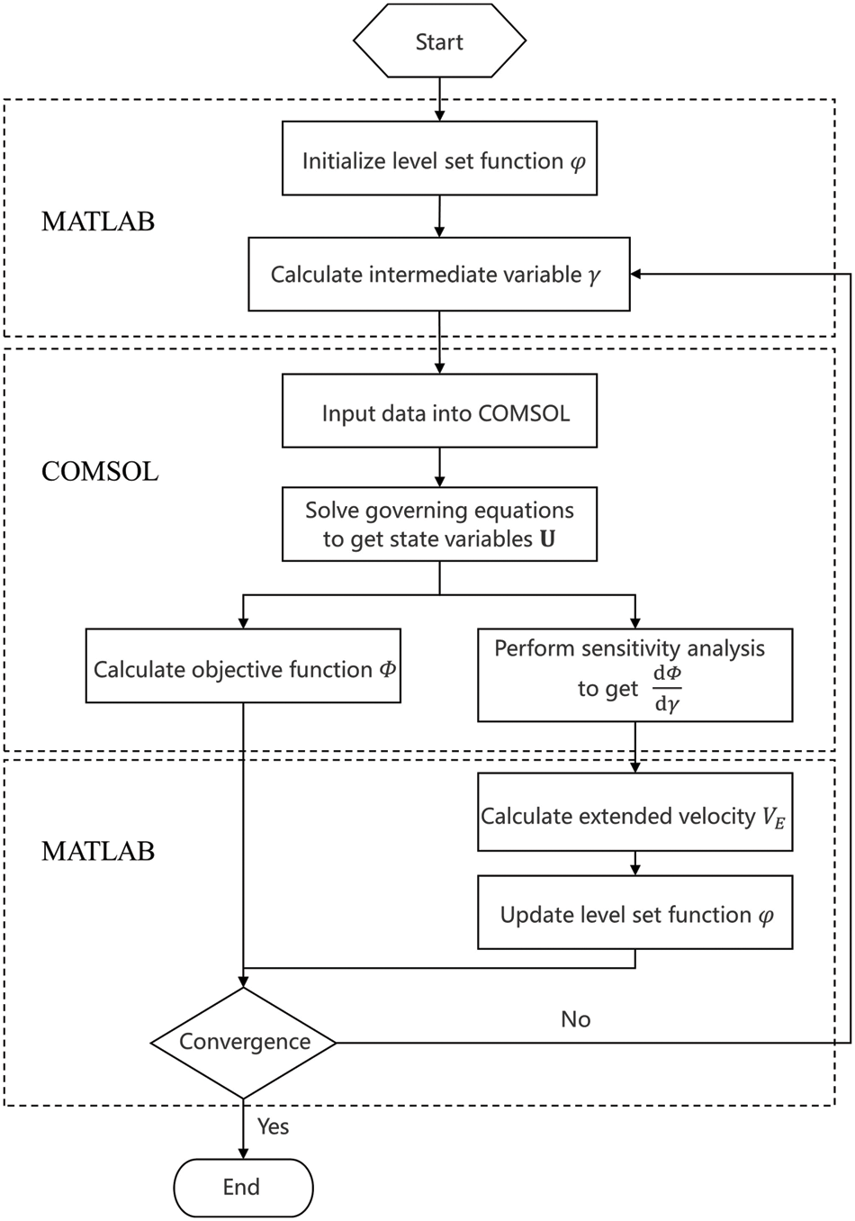
Figure 4: The flow chart of the optimization procedure
We edit codes in MATLAB, and then call the commands in COMSOL Multiphysics to solve the Navier-Stokes equation and adjoint equations. In the current work, the essential idea of the 88-line MATLAB code presented by Wei et al. [35] for the compliance minimization problem and the local optimality condition [62,63] are adopted here and extended to the fluid topology optimization problem. In addition, the design domain is discretized by the linear rectangle elements and triangle elements in 2D cases and tetrahedron elements in 3D cases.
In this section, several numerical examples are presented to demonstrate the effectiveness of the proposed method. The numerical examples in Section 5.1 do not consider gravity, and the body force
where
where D denotes a characteristic length scale which is set to 1 in this paper.
5.1 Numerical Examples without Gravity
The first numerical example is to study the topology optimization of a double pipe problem, in which the design domain is discretized by structured mesh and unstructured mesh, respectively. The design domain and boundary conditions information are shown in Fig. 5. The prescribed fluid volume fraction of the optimization problem is 0.35, and the Reynolds number is set to
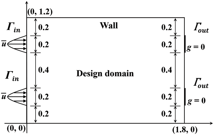
Figure 5: Design domain and boundary conditions for the double pipe problem
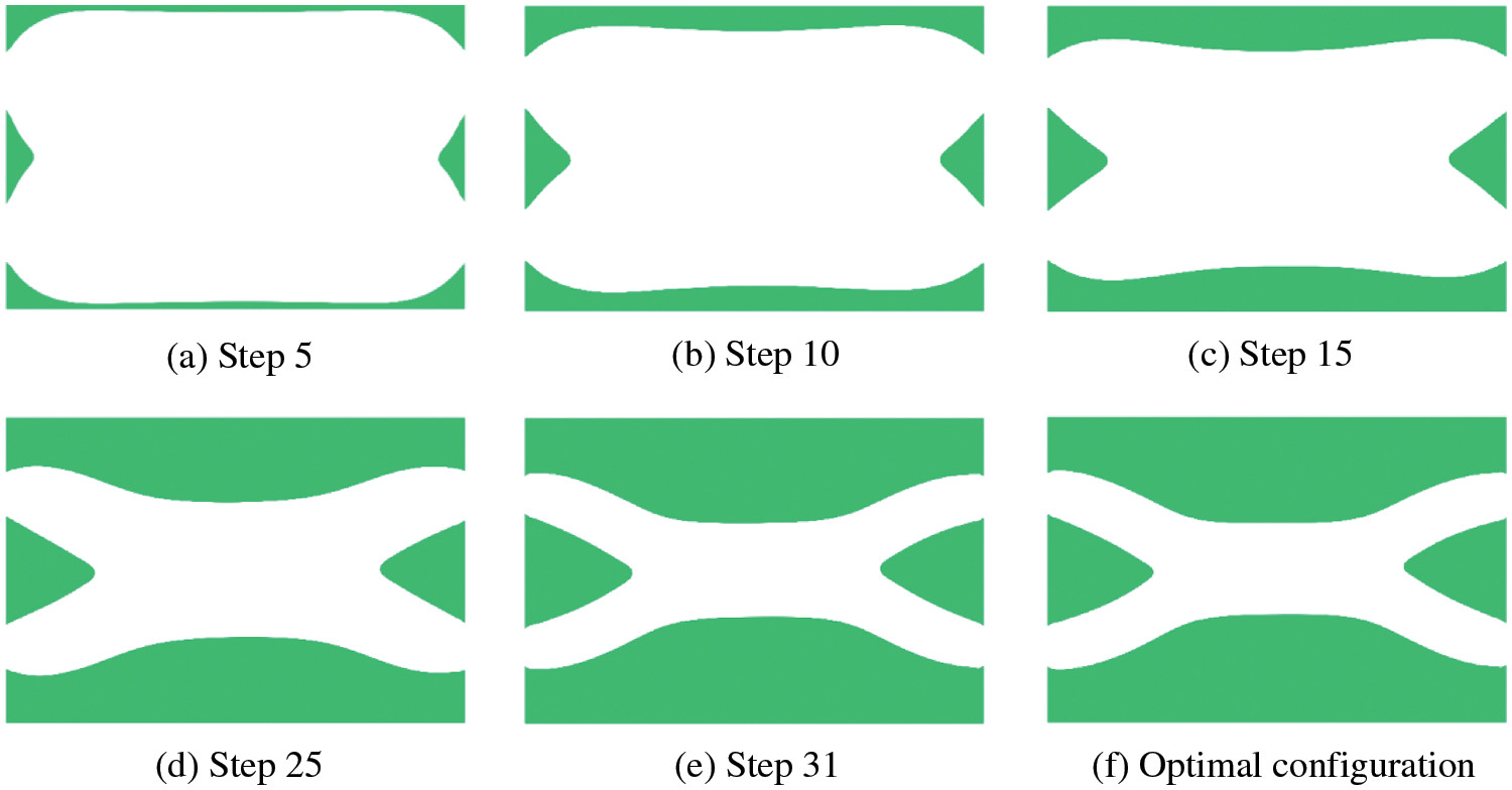
Figure 6: Optimization history for the double pipe problem
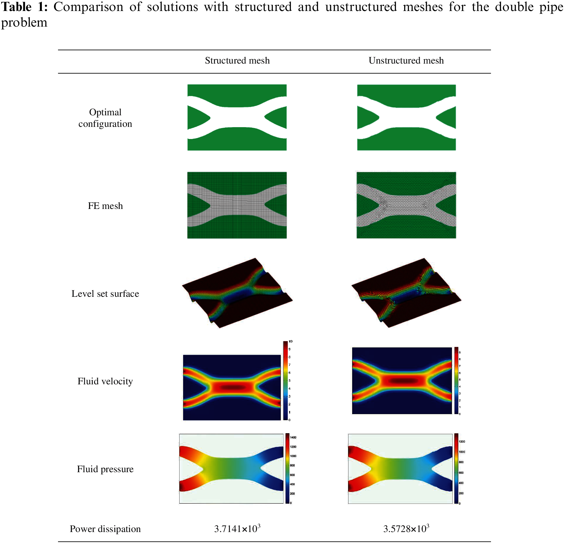
The optimal solutions for different meshes of the double pipe problem are shown in Table 1. The optimal configurations in the first row of Table 1 display the coherence between the structured quadrilateral meshes and the unstructured triangular meshes. Due to the use of unstructured mesh, a small portion of the boundary is not sufficiently smooth, which may be further improved by using the polygonal elements [58,69]. However, the result for unstructured meshed has only slight differences from that of structured meshes. Further, Fluid velocity fields, fluid pressure fields, and the power dissipation values show negligible differences. By comparing the results of two different types of mesh, the method proposed in this paper is proven to apply to unstructured grids and works well.
5.1.2 Four-Terminal Device with Different Reynolds Numbers
In the second numerical example, a four-terminal device is considered to minimize power dissipation with a prescribed fluid volume fraction which is similar to the problems proposed by Borrvall et al. [15], Gersborg-Hansen et al. [17], Olesen et al. [18] and Dai et al. [48]. The design domain and boundary conditions information are shown in Fig. 7. The design domain is discretized by 100 × 70 rectangular elements and the fluid volume fraction is 0.4. To study the effect of the Reynolds number on the optimal configuration, the Reynolds number is set as
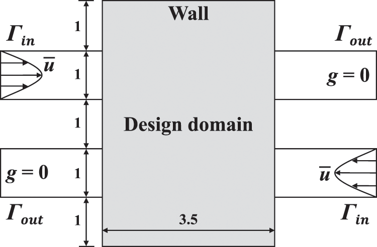
Figure 7: Design domain and boundary conditions for the four-terminal device problem
Fig. 8 displays the optimal configurations for different Reynolds numbers, in which the optimal four-terminal device has two bending channels for the flow with a small Reynolds number, while the optimal four-terminal device with a large Reynolds number has two parallel straight channels. With the increase of the Reynolds number, the fluid power dissipation caused by the bending channels increases. When the inertia effect dominates, a large velocity gradient appears in the bending channels, and this increases power dissipation compared to the low Reynolds number case. Therefore, the optimal four-terminal device has two parallel straight channels for large Reynolds number flow. Fig. 9 displays the convergence curves of power dissipation and volume fraction when the Reynolds number is equal to 20.
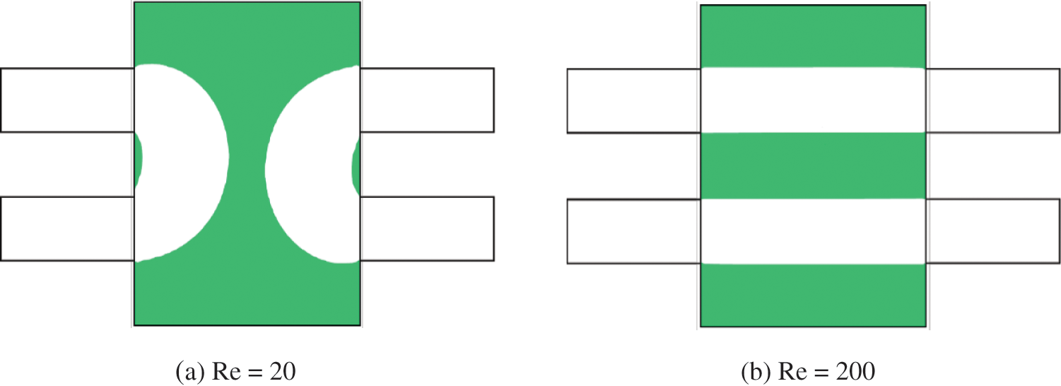
Figure 8: Optimal configurations corresponding to different Reynolds numbers for the four-terminal device problem
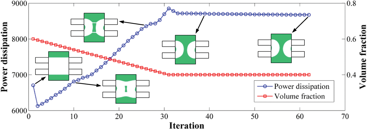
Figure 9: Convergence curves of power dissipation and volume fraction when the Reynolds number is equal to 20 for the four-terminal device problem
In addition, Yaji et al. [70] have proven that the value of the Reynolds number affects the channel’s configuration, and the curvature radius of the channel decrease as the Reynolds number is increased. Furthermore, we study the double pipe problem in Section 5.1.1 at different Reynolds numbers, which is started from an initial region that is completely fluid. The prescribed fluid volume fraction of the optimization problem is 1/3, and the Reynolds numbers are set to
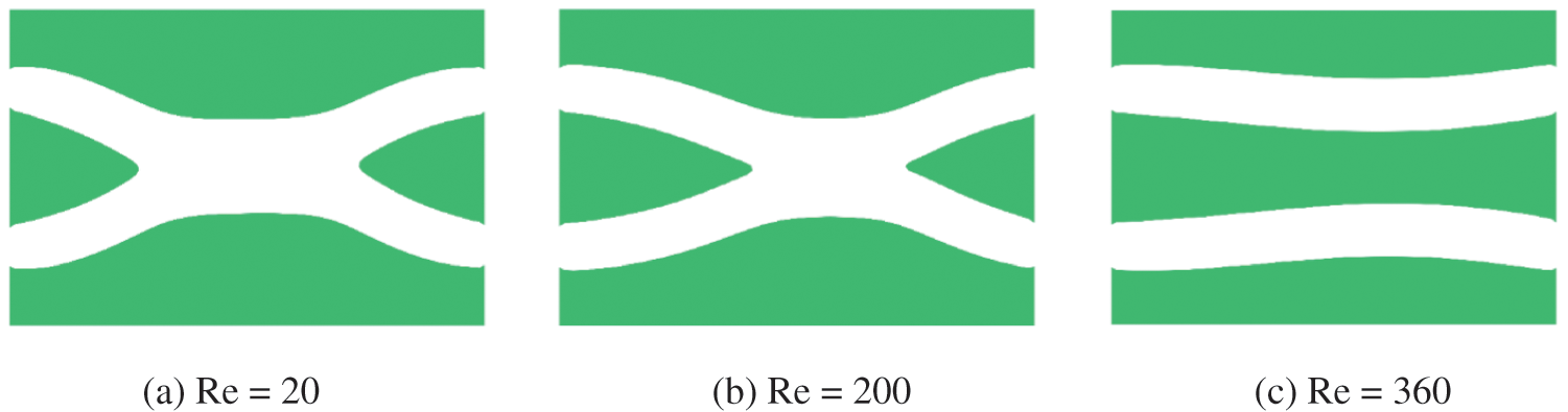
Figure 10: Optimal configurations corresponding to different Reynolds numbers for the double pipe problem
Theoretically, when the Reynolds number is equal to 360, the optimal configuration should be two parallel straight channels, which minimizes power dissipation. However, when the initial design as shown in Fig. 11a is adopted, two parallel straight channels can be obtained as shown in Fig. 11b. The power dissipation in Figs. 10c and 11b are 8.9648 × 10⁶ and 7.9960 × 10⁶, respectively. Therefore, the proposed method is sensitive to the initial design for some problems.
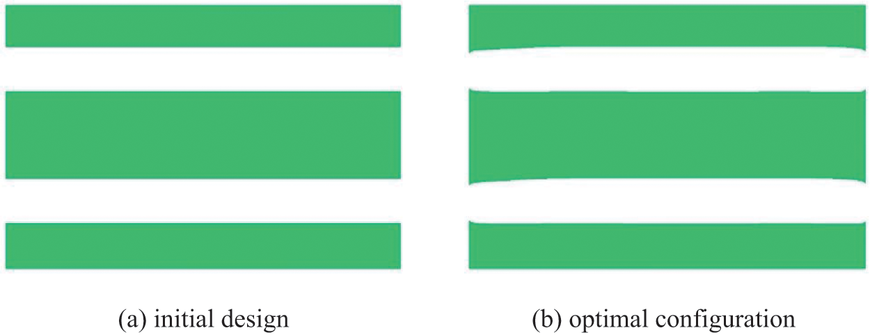
Figure 11: Another initial design and corresponding optimal configuration when Reynolds number is equal to 360
5.1.3 Rectangular Splitter with Different Initial Designs
The third example is the topology optimization of a rectangular splitter problem, considering three different initial designs to examine the dependency of the method proposed in this paper on the initial design. Fig. 12 shows the design domain and boundary conditions. The objective is to minimize the power dissipation in optimal configuration between the inlet and the outlets. The design domain of the rectangular splitter is discretized by 60 × 100 rectangular elements. The prescribed fluid volume fraction of the optimization problem is 0.5, and the Reynolds number is set to
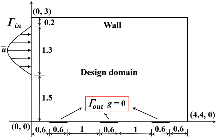
Figure 12: Design domain and boundary conditions for the rectangular splitter problem
Table 2 exhibits three different initial designs and several iterative steps in their corresponding optimization procedures. Although the three initial designs are different, the optimal configurations obtained are roughly the same, and any two values of the objective function differ by less than 5%. Therefore, the method proposed in this paper is not sensitive to the initial design. In addition, the evolution histories of contours corresponding to three initial designs are shown in Table 2. So, here’s what we can see is optimal configurations have clear and smooth boundaries in the optimization procedure, which demonstrates that the method proposed in this paper can deal with geometric boundary and topology change problems well. Fig. 13 gives the convergence curves of the objective function and the fluid volume fraction for case 3.
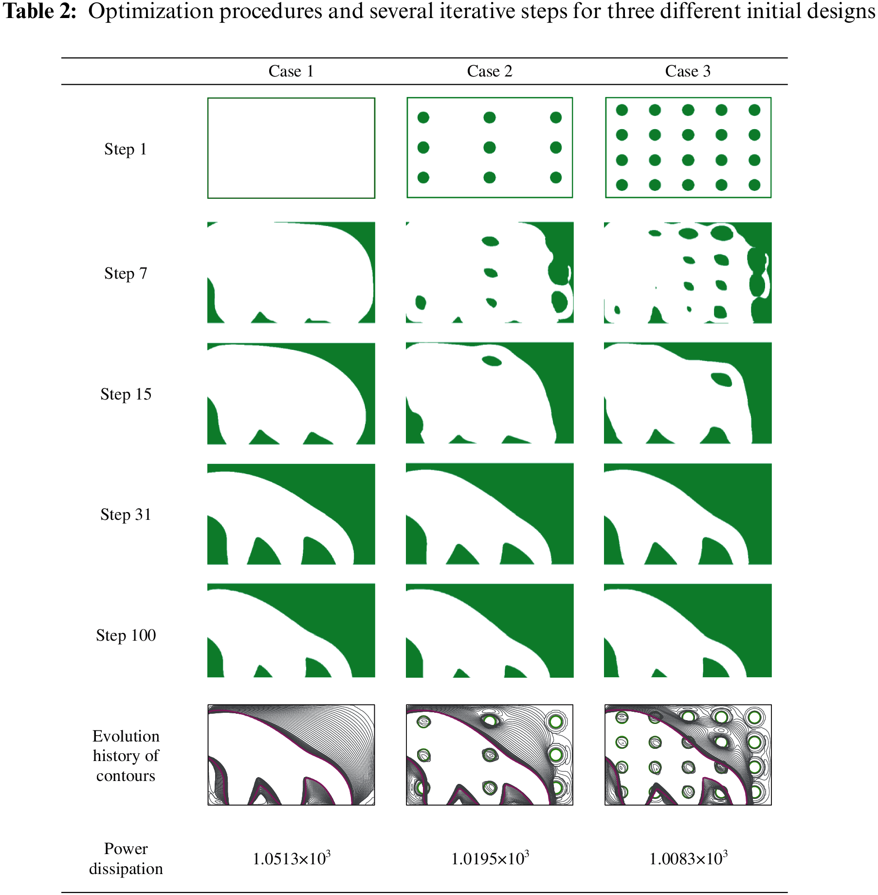
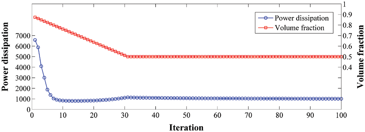
Figure 13: Convergence curves of power dissipation and volume fraction of case 3 for the rectangular splitter problem
This numerical example is a Z-pipe problem that has an irregular design domain. The design domain and boundary conditions are shown in Fig. 14a. The design domain is discretized by 4216 unstructured triangular elements and the Reynolds number is set to
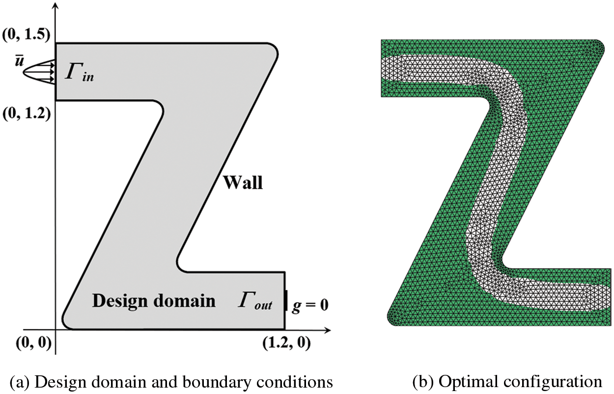
Figure 14: Design domains, boundary conditions and optimal configuration for the Z-pipe problem
The first numerical example in 3D is a bend pipe problem which is used to demonstrate that the proposed method can be successfully applied to three-dimensional problems. The design domain of the bend pipe problem is shown in Fig. 15, which is discretized by 161,851 tetrahedron elements. Note the types of boundary conditions for the inlets and outlets are consistent with the 2D numerical examples, but the initial velocities of the inlet are uniform flows rather than parabolic flows. The Reynolds number is set to
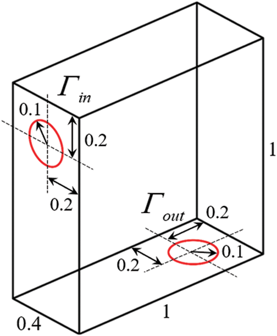
Figure 15: Design domain for the bend pipe problem
Fig. 16 shows the optimal configurations in different directions for the bend pipe problem. The optimal configuration is a bent pipe connecting the inlet and outlet. However, the surfaces of the optimal configurations are not smooth due to the unstructured mesh, i.e., the tetrahedron element. A refinement method [71] is adopted here to obtain smooth results. Refined mesh schemes with 874,387 tetrahedron elements are adopted to smooth the surfaces of optimal configuration, the smooth results are shown in Fig. 17. Therefore, this numerical example demonstrates that the proposed method is feasible in three-dimensional and smooth results can be obtained with a refinement method [71].
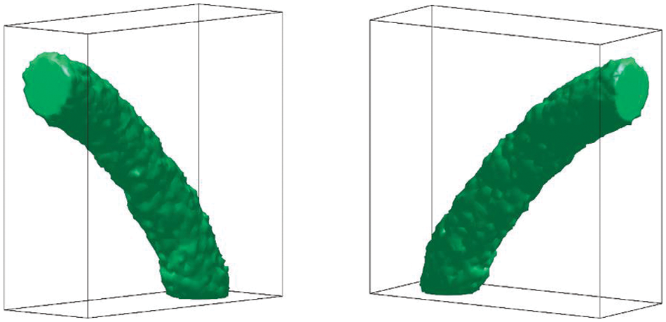
Figure 16: Optimal configurations in different directions for the bend pipe problem
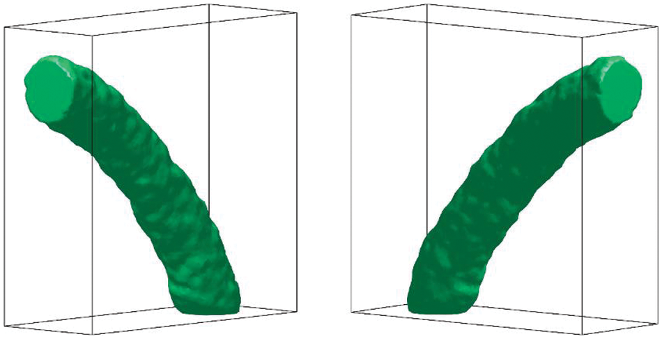
Figure 17: Smooth optimal configurations in different directions for the bend pipe problem
5.1.6 Multi-Outlet Terminal in 3D
The second numerical example in 3D is a multi-outlet and its design domain is shown in Fig. 18, which is discretized by 178,562 tetrahedron elements. The initial velocities of the inlet are uniform flows rather than parabolic flows. The Reynolds number is set to
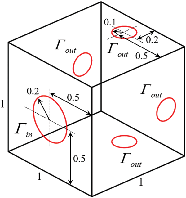
Figure 18: Design domain for the multi-outlet problem
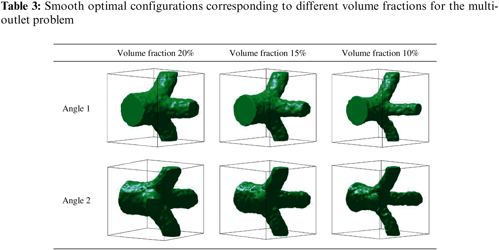
Consistent with the bend pipe problem, the refinement method [71] is adopted to obtain smooth results. Refined mesh schemes with 2,192,849 tetrahedron elements are adopted to smooth the surfaces of optimal configuration, the smooth results corresponding to different volume fractions are shown in Table 3. With the decrease of volume fraction, the pipes become thinner. In addition, it can be seen that when the volume fraction is 10%, the pipe on the right side is thinner than those on the other sides, the reason may be the finite element mesh dividing the design domain is unstructured.
5.2 Numerical Examples with Gravity
In this numerical example, the simplest body force, e.g., gravity, is considered in the Navier-Stokes equations. Comparing the optimal fluid channels with and without gravity, the effectiveness of the proposed method in considering gravity is studied. The design domain and boundary conditions are shown in Fig. 19. Note that the inlet is the middle third of the length on the left side while the outlet is the entire length on the right side. The design domain is discretized by 3600 rectangle elements and the Reynolds number is set to
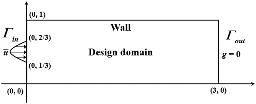
Figure 19: Design domain and boundary conditions for the horizontal channel in gravity problem
Fig. 20 shows the Optimal configurations for the horizontal channel with and without gravity. It can be concluded that gravity causes the bending horizontal channel by comparing the optimal configuration without gravity. Extra work is applied to the fluid by gravity, causing the fluid to bend in the direction of gravity, just as water flows down from a high place, which is consistent with reality. And it also shows the effectiveness of the proposed method in the fluid with gravity. In addition, we find a phenomenon where two small curved angles appear at the fluid inlets, as shown in Fig. 20. It can be attributed that the artificial friction force is added to the Navier-Stokes equation to distinguish the solid and fluid regions, the impermeability in the solid region is a large but finite positive constant and the velocity in the solid region tend to zero but not equal to zero; the initial velocity at the inlet has a parabolic shape, and the velocities at the upper and lower parts of the inlet are close to zero, so they can flow through the small curved angles.
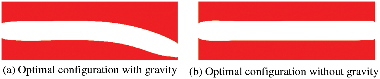
Figure 20: Optimal configurations for the horizontal channel with and without gravity
This numerical example extends the proposed method with gravity to the 3D case. The design domain of the splitter is shown in Fig. 21, which is discretized by 169,510 tetrahedron elements. The Reynolds number is set to
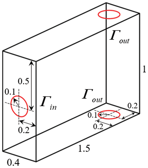
Figure 21: Design domain for the splitter problem
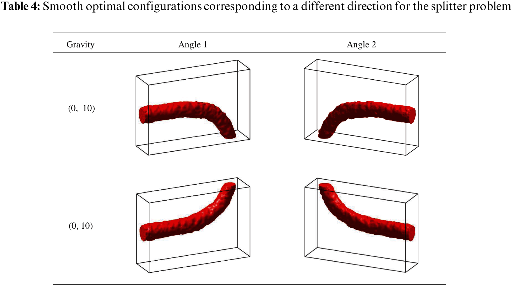
Refined mesh schemes with 1,592,844 tetrahedron elements are adopted to smooth the surfaces of optimal configuration, the smooth results corresponding to different directions are shown in Table 4. When the direction of gravity is downward, the fluid flows downward and the lower outlet is chosen, otherwise, the fluid flows upward and the upper outlet is chosen. It can be seen that when the direction of gravity is changed, the bending direction of the flow channel will change accordingly. It also further verifies the influence of gravity on the optimal configuration in a 3D case.
In this paper, we employ the parameterized level set method using basis functions to study the topology optimization problems of steady-state incompressible Navier-Stokes flow. The intermediate variable
In Section 5.1, six numerical examples demonstrate the proposed method has flexibility and effectiveness in different kinds of design domains and mesh categories. The four-terminal device examples in Section 5.1.2 give similar observations as the research of others. That is the Reynolds number affects the shape of the optimal Configuration, and the larger the Reynolds number, the more inclined to obtain straight flow channels. In Section 5.2, two numerical examples of the horizontal channel in gravity illustrate the effectiveness of the proposed method in channel optimal design problems with gravity by comparing the optimal configuration with and without gravity. In addition, the proposed method is successfully applied to three-dimensional design problems and relatively smooth results can be obtained through the refinement method, so the proposed method has the potential in solving practical engineering problems.
However, the surface of the 3D results shown in this paper is still a little rough, which can be further improved by refining mesh and adopting other post-processing methods. Besides, the current work only considers constant body force (e.g., gravity), and it is necessary to be extended to fluid flow problems with other kinds of physical body forces in the future, such as centrifugal force and Coriolis force.
Funding Statement: This research was supported by the National Natural Science Foundation of China (Grant No. 12072114), the National Key Research and Development Plan (Grant No. 2020YFB1709401), and the Guangdong Provincial Key Laboratory of Modern Civil Engineering Technology (2021B1212040003).
Conflicts of Interest: The authors declare that they have no conflicts of interest to report regarding the present study.
References
1. Liu, B., Yan, X., Li, Y., Zhou, S., Huang, X. (2021). Multi-material topology optimization of structures using an ordered ersatz material model. Computer Modeling in Engineering & Sciences, 128(2), 523–540. DOI 10.32604/cmes.2021.017211. [Google Scholar] [CrossRef]
2. Allaire, G., Bonnetier, E., Francfort, G., Jouve, F. (1997). Shape optimization by the homogenization method. Numerische Mathematik, 76(1), 27–68. DOI 10.1007/s002110050253. [Google Scholar] [CrossRef]
3. Bendsøe, M. P., Kikuchi, N. (1988). Generating optimal topologies in structural design using a homogenization method. Computer Methods in Applied Mechanics and Engineering, 71(2), 197–224. DOI 10.1016/0045-7825(88)90086-2. [Google Scholar] [CrossRef]
4. Bendsøe, M. P., Sigmund, O. (1999). Material interpolation schemes in topology optimization. Archive of Applied Mechanics, 69(9), 635–654. [Google Scholar]
5. Rozvany, G. I. (2001). Aims, scope, methods, history and unified terminology of computer-aided topology optimization in structural mechanics. Structural and Multidisciplinary Optimization, 21(2), 90–108. DOI 10.1007/s001580050174. [Google Scholar] [CrossRef]
6. Xie, Y. M., Steven, G. P. (1993). A simple evolutionary procedure for structural optimization. Computers & Structures, 49(5), 885–896. DOI 10.1016/0045-7949(93)90035-C. [Google Scholar] [CrossRef]
7. Querin, O. M., Steven, G. P., Xie, Y. M. (1998). Evolutionary structural optimisation (ESO) using a bidirectional algorithm. Engineering Computations, 15(8), 1031–1048. DOI 10.1108/02644409810244129. [Google Scholar] [CrossRef]
8. Huang, X., Xie, Y. M. (2008). Optimal design of periodic structures using evolutionary topology optimization. Structural and Multidisciplinary Optimization, 36(6), 597–606. DOI 10.1007/s00158-007-0196-1. [Google Scholar] [CrossRef]
9. Wang, M. Y., Wang, X., Guo, D. (2003). A level set method for structural topology optimization. Computer Methods in Applied Mechanics and Engineering, 192(1–2), 227–246. DOI 10.1016/S0045-7825(02)00559-5. [Google Scholar] [CrossRef]
10. Wang, M. Y., Wang, X. (2004). PDE-driven level sets, shape sensitivity and curvature flow for structural topology optimization. Computer Modeling in Engineering & Sciences, 6(4), 373–396. DOI 10.3970/cmes.2004.006.373. [Google Scholar] [CrossRef]
11. Allaire, G., Jouve, F., Toader, A. M. (2004). Structural optimization using sensitivity analysis and a level-set method. Journal of Computational Physics, 194(1), 363–393. DOI 10.1016/j.jcp.2003.09.032. [Google Scholar] [CrossRef]
12. Xing, X., Wei, P., Wang, M. Y. (2010). A finite element-based level set method for structural optimization. International Journal for Numerical Methods in Engineering, 82(7), 805–842. DOI 10.1002/nme.2785. [Google Scholar] [CrossRef]
13. Zhang, W., Yuan, J., Zhang, J., Guo, X. (2016). A new topology optimization approach based on moving morphable components (MMC) and the ersatz material model. Structural and Multidisciplinary Optimization, 53(6), 1243–1260. DOI 10.1007/s00158-015-1372-3. [Google Scholar] [CrossRef]
14. Zhang, W., Li, D., Kang, P., Guo, X., Youn, S. K. (2020). Explicit topology optimization using IGA-based moving morphable void (MMV) approach. Computer Methods in Applied Mechanics and Engineering, 360, 112685. DOI 10.1016/j.cma.2019.112685. [Google Scholar] [CrossRef]
15. Borrvall, T., Petersson, J. (2003). Topology optimization of fluids in stokes flow. International Journal for Numerical Methods in Fluids, 41(1), 77–107. DOI 10.1002/(ISSN)1097-0363. [Google Scholar] [CrossRef]
16. Gersborg-Hansen, A. (2003). Topology optimization of incompressible Newtonian flows at moderate Reynolds numbers (Master Thesis). Technical University of Denmark, Denmark. [Google Scholar]
17. Gersborg-Hansen, A., Sigmund, O., Haber, R. B. (2005). Topology optimization of channel flow problems. Structural and Multidisciplinary Optimization, 30(3), 181–192. DOI 10.1007/s00158-004-0508-7. [Google Scholar] [CrossRef]
18. Olesen, L. H., Okkels, F., Bruus, H. (2006). A high-level programming-language implementation of topology optimization applied to steady-state navier–stokes flow. International Journal for Numerical Methods in Engineering, 65(7), 975–1001. DOI 10.1002/(ISSN)1097-0207. [Google Scholar] [CrossRef]
19. Pironnea, O. (1973). On optimum profiles in stokes flow. Journal of Fluid Mechanics, 59(1), 117–128. DOI 10.1017/S002211207300145X. [Google Scholar] [CrossRef]
20. Pironnea, O. (1974). On optimum design in fluid mechanics. Journal of Fluid Mechanics, 64(1), 97–110. DOI 10.1017/S0022112074002023. [Google Scholar] [CrossRef]
21. Sigmund, O., Gersborg-Hansen, A., Haber, R. (2003). Topology optimization for multiphysics problems: A future FEMLAB application? Nordic MATLAB Conference, pp. 237–242. Søborg, Denmark. [Google Scholar]
22. Guest, J. K., Prévost, J. H. (2006). Topology optimization of creeping fluid flows using a Darcy–Stokes finite element. International Journal for Numerical Methods in Engineering, 66(3), 461–484. DOI 10.1002/(ISSN)1097-0207. [Google Scholar] [CrossRef]
23. Liu, Z., Gao, Q., Zhang, P., Xuan, M., Wu, Y. (2011). Topology optimization of fluid channels with flow rate equality constraints. Structural and Multidisciplinary Optimization, 44(1), 31–37. DOI 10.1007/s00158-010-0591-x. [Google Scholar] [CrossRef]
24. Deng, Y., Liu, Z., Zhang, P., Liu, Y., Wu, Y. (2011). Topology optimization of unsteady incompressible Navier–Stokes flows. Journal of Computational Physics, 230(17), 6688–6708. DOI 10.1016/j.jcp.2011.05.004. [Google Scholar] [CrossRef]
25. Deng, Y., Liu, Z., Wu, Y. (2013). Topology optimization of steady and unsteady incompressible Navier–Stokes flows driven by body forces. Structural and Multidisciplinary Optimization, 47(4), 555–570. DOI 10.1007/s00158-012-0847-8. [Google Scholar] [CrossRef]
26. Pereira, A., Talischi, C., Paulino, G. H., Menezes, M. I. F., Carvalho, S. M. (2016). Fluid flow topology optimization in PolyTop: Stability and computational implementation. Structural and Multidisciplinary Optimization, 54(5), 1345–1364. DOI 10.1007/s00158-014-1182-z. [Google Scholar] [CrossRef]
27. Talischi, C., Paulino, G. H., Pereira, A., Menezes, I. F. (2012). PolyTop: A matlab implementation of a general topology optimization framework using unstructured polygonal finite element meshes. Structural and Multidisciplinary Optimization, 45(3), 329–357. DOI 10.1007/s00158-011-0696-x. [Google Scholar] [CrossRef]
28. Shen, C., Hou, L., Zhang, E., Lin, J. (2018). Topology optimization of three-phase interpolation models in Darcy-Stokes flow. Structural and Multidisciplinary Optimization, 57(4), 1663–1677. DOI 10.1007/s00158-017-1836-8. [Google Scholar] [CrossRef]
29. Malladi, R., Sethian, J. A. (1995). Image processing via level set curvature flow. Proceedings of the National Academy of Sciences, 92(15), 7046–7050. DOI 10.1073/pnas.92.15.7046. [Google Scholar] [CrossRef]
30. Chopp, D. L. (1993). Computing minimal surfaces via level set curvature flow. Journal of Computational Physics, 106(1), 77–91. DOI 10.1006/jcph.1993.1092. [Google Scholar] [CrossRef]
31. Sethian, J. A., Wiegmann, A. (2000). Structural boundary design via level set and immersed interface methods. Journal of Computational Physics, 163(2), 489–528. DOI 10.1006/jcph.2000.6581. [Google Scholar] [CrossRef]
32. Sussman, M., Smereka, P., Osher, S. (1994). A level set approach for computing solutions to incompressible two-phase flow. Journal of Computational Physics, 114(1), 146–159. DOI 10.1006/jcph.1994.1155. [Google Scholar] [CrossRef]
33. Zhao, H. K., Chan, T., Merriman, B., Osher, S. (1996). A variational level set approach to multiphase motion. Journal of Computational Physics, 127(1), 179–195. DOI 10.1006/jcph.1996.0167. [Google Scholar] [CrossRef]
34. Osher, S., Sethian, J. A. (1988). Fronts propagating with curvature-dependent speed: Algorithms based on Hamilton-Jacobi formulations. Journal of Computational Physics, 79(1), 12–49. DOI 10.1016/0021-9991(88)90002-2. [Google Scholar] [CrossRef]
35. Wei, P., Li, Z., Li, X., Wang, M. Y. (2018). An 88-line MATLAB code for the parameterized level set method based topology optimization using radial basis functions. Structural and Multidisciplinary Optimization, 58(2), 831–849. DOI 10.1007/s00158-018-1904-8. [Google Scholar] [CrossRef]
36. Zhou, S., Li, Q. (2008). A variational level set method for the topology optimization of steady-state Navier–Stokes flow. Journal of Computational Physics, 227(24), 10178–10195. DOI 10.1016/j.jcp.2008.08.022. [Google Scholar] [CrossRef]
37. Duan, X., Ma, Y., Zhang, R. (2008). Optimal shape control of fluid flow using variational level set method. Physics Letters A, 372(9), 1374–1379. DOI 10.1016/j.physleta.2007.09.070. [Google Scholar] [CrossRef]
38. Duan, X., Ma, Y., Zhang, R. (2008). Shape-topology optimization of stokes flow via variational level set method. Applied Mathematics and Computation, 202(1), 200–209. DOI 10.1016/j.amc.2008.02.014. [Google Scholar] [CrossRef]
39. Duan, X., Ma, Y., Zhang, R. (2008). Shape-topology optimization for Navier–Stokes problem using variational level set method. Journal of Computational and Applied Mathematics, 222(2), 487–499. DOI 10.1016/j.cam.2007.11.016. [Google Scholar] [CrossRef]
40. Challis, V. J., Guest, J. K. (2009). Level set topology optimization of fluids in stokes flow. International Journal for Numerical Methods in Engineering, 79(10), 1284–1308. DOI 10.1002/nme.2616. [Google Scholar] [CrossRef]
41. Pingen, G., Waidmann, M., Evgrafov, A., Maute, K. (2010). A parametric level-set approach for topology optimization of flow domains. Structural and Multidisciplinary Optimization, 41(1), 117–131. DOI 10.1007/s00158-009-0405-1. [Google Scholar] [CrossRef]
42. Kreissl, S., Pingen, G., Maute, K. (2011). An explicit level set approach for generalized shape optimization of fluids with the lattice Boltzmann method. International Journal for Numerical Methods in Fluids, 65(5), 496–519. DOI 10.1002/fld.2193. [Google Scholar] [CrossRef]
43. Kreissl, S., Maute, K. (2012). Levelset based fluid topology optimization using the extended finite element method. Structural and Multidisciplinary Optimization, 46(3), 311–326. DOI 10.1007/s00158-012-0782-8. [Google Scholar] [CrossRef]
44. Deng, Y., Liu, Z., Wu, J., Wu, Y. (2013). Topology optimization of steady navier–stokes flow with body force. Computer Methods in Applied Mechanics and Engineering, 255, 306–321. DOI 10.1016/j.cma.2012.11.015. [Google Scholar] [CrossRef]
45. Zhang, B., Liu, X. (2015). Topology optimization study of arterial bypass configurations using the level set method. Structural and Multidisciplinary Optimization, 51(3), 773–798. DOI 10.1007/s00158-014-1175-y. [Google Scholar] [CrossRef]
46. Deng, Y., Liu, Z., Wu, Y. (2017). Topology optimization of capillary, two-phase flow problems. Communications in Computational Physics, 22(5), 1413–1438. DOI 10.4208/cicp.OA-2017-0003. [Google Scholar] [CrossRef]
47. Koch, J. R. L., Papoutsis-Kiachagias, E. M., Giannakoglou, K. C. (2017). Transition from adjoint level set topology to shape optimization for 2D fluid mechanics. Computers & Fluids, 150, 123–138. DOI 10.1016/j.compfluid.2017.04.001. [Google Scholar] [CrossRef]
48. Dai, X., Zhang, C., Zhang, Y., Gulliksson, M. (2018). Topology optimization of steady Navier-Stokes flow via a piecewise constant level set method. Structural and Multidisciplinary Optimization, 57(6), 2193–2203. DOI 10.1007/s00158-017-1850-x. [Google Scholar] [CrossRef]
49. Duan, X., Dang, Y., Lu, J. (2020). A variational level set method for topology optimization problems in Navier-Stokes flow. IEEE Access, 8, 48697–48706. DOI 10.1109/Access.6287639. [Google Scholar] [CrossRef]
50. Nguyen, T., Isakari, H., Takahashi, T., Yaji, K., Yoshino, M. et al. (2020). Level-set based topology optimization of transient flow using lattice Boltzmann method considering an oscillating flow condition. Computers & Mathematics with Applications, 80(1), 82–108. DOI 10.1016/j.camwa.2020.03.003. [Google Scholar] [CrossRef]
51. Kubo, S., Koguchi, A., Yaji, K., Yamada, T., Izui, K. et al. (2021). Level set-based topology optimization for two dimensional turbulent flow using an immersed boundary method. Journal of Computational Physics, 446, 110630. DOI 10.1016/j.jcp.2021.110630. [Google Scholar] [CrossRef]
52. Cai, H., Guo, K., Liu, H., Liu, C., Feng, A. (2021). Derivative-free level-set-based multi-objective topology optimization of flow channel designs using lattice Boltzmann method. Chemical Engineering Science, 231, 116323. DOI 10.1016/j.ces.2020.116323. [Google Scholar] [CrossRef]
53. Sethian, J. A. (1999). Level set methods and fast marching methods: Evolving interfaces in computational geometry, fluid mechanics, computer vision, and materials science, vol. 3. UK: Cambridge University Press. [Google Scholar]
54. Osher, S., Fedkiw, R. (2002). Level set methods and dynamic implicit surfaces, vol. 153. Berlin, Heidelberg: Springer Science & Business Media. [Google Scholar]
55. Wang, S., Wang, M. Y. (2006). Radial basis functions and level set method for structural topology optimization. International Journal for Numerical Methods in Engineering, 65(12), 2060–2090. DOI 10.1002/(ISSN)1097-0207. [Google Scholar] [CrossRef]
56. Wang, S., Wang, M. (2006). Structural shape and topology optimization using an implicit free boundary parametrization method. Computer Modeling in Engineering & Sciences, 13(2), 119–148. DOI 10.3970/cmes.2006.013.119. [Google Scholar] [CrossRef]
57. Wang, S. Y., Lim, K. M., Khoo, B. C., Wang, M. Y. (2007). An extended level set method for shape and topology optimization. Journal of Computational Physics, 221(1), 395–421. DOI 10.1016/j.jcp.2006.06.029. [Google Scholar] [CrossRef]
58. Wei, P., Paulino, G. H. (2020). A parameterized level set method combined with polygonal finite elements in topology optimization. Structural and Multidisciplinary Optimization, 61(5), 1913–1928. DOI 10.1007/s00158-019-02444-y. [Google Scholar] [CrossRef]
59. Liu, H., Wei, P., Wang, M. Y. (2022). CPU parallel-based adaptive parameterized level set method for large-scale structural topology optimization. Structural and Multidisciplinary Optimization, 65(1), 1–15. DOI 10.1007/s00158-021-03086-9. [Google Scholar] [CrossRef]
60. Lin, H., Liu, H., Wei, P. (2022). A parallel parameterized level set topology optimization framework for large-scale structures with unstructured meshes. Computer Methods in Applied Mechanics and Engineering, 397, 115112. DOI 10.1016/j.cma.2022.115112. [Google Scholar] [CrossRef]
61. Kansa, E. J., Power, H., Fasshauer, G. E., Ling, L. (2004). A volumetric integral radial basis function method for time-dependent partial differential equations. I. Formulation. Engineering Analysis with Boundary Elements, 28(10), 1191–1206. DOI 10.1016/j.enganabound.2004.01.004. [Google Scholar] [CrossRef]
62. Jiang, L., Chen, S., Jiao, X. (2018). Parametric shape and topology optimization: A new level set approach based on cardinal basis functions. International Journal for Numerical Methods in Engineering, 114(1), 66–87. DOI 10.1002/nme.5733. [Google Scholar] [CrossRef]
63. Wei, P., Yang, Y., Chen, S., Wang, M. Y. (2021). A study on basis functions of the parameterized level set method for topology optimization of continuums. Journal of Mechanical Design, 143(4). DOI 10.1115/1.4047900. [Google Scholar] [CrossRef]
64. Wei, P., Wang, W., Yang, Y., Wang, M. Y. (2020). Level set band method: A combination of density-based and level set methods for the topology optimization of continuums. Frontiers of Mechanical Engineering, 15(3), 390–405. DOI 10.1007/s11465-020-0588-0. [Google Scholar] [CrossRef]
65. Duan, X., Qin, X., Li, F. (2016). Topology optimization of stokes flow using an implicit coupled level set method. Applied Mathematical Modelling, 40(9–10), 5431–5441. DOI 10.1016/j.apm.2015.12.040. [Google Scholar] [CrossRef]
66. COMSOL AB (2008). COMSOL multiphysics reference guide for COMSOL 3.5. In: Advanced solver topics, pp. 533–543. Stockholm: COMSOL AB. [Google Scholar]
67. Zhang, S., Li, P., Zhong, Y., Xiang, J. (2014). Structural topology optimization based on the level set method using COMSOL. Computer Modeling in Engineering & Sciences, 101(1), 17–31. DOI 10.3970/cmes.2014.101.017. [Google Scholar] [CrossRef]
68. Qiu, G., Wei, P., Huang, P., Pan, M. (2021). Topology optimization design of a microchannel plate based on velocity distribution. Chemical Engineering & Technology, 44(4), 681–689. DOI 10.1002/ceat.202000555. [Google Scholar] [CrossRef]
69. Lee, C., Natarajan, S., Kee, S., Yee, J. (2022). A cell-based linear smoothed finite element method for polygonal topology optimization. Computer Modeling in Engineering & Sciences, 131(3), 1615–1634. DOI 10.32604/cmes.2022.020377. [Google Scholar] [CrossRef]
70. Yaji, K., Yamada, T., Yoshino, M., Matsumoto, T., Izui, K. et al. (2014). Topology optimization using the lattice Boltzmann method incorporating level set boundary expressions. Journal of Computational Physics, 274, 158–181. DOI 10.1016/j.jcp.2014.06.004. [Google Scholar] [CrossRef]
71. Wei, P., Liu, Y., Li, Z. (2020). A multi-discretization scheme for topology optimization based on the parameterized level set method. International Journal for Simulation and Multidisciplinary Design Optimization, 11, 3. DOI 10.1051/smdo/2019019. [Google Scholar] [CrossRef]
Appendix A
The derivation of
where
Note that, the sensitivity of the state variables with respect to the design variables,
Therefore, the total derivative of the augmented objective function with respect to the intermediate variable can be written as follows:
Since the state solution at each loop will always make the residual vector
Therefore, the total derivative of the objective function with respect to the intermediate variable is:
It should be noted that the above procedures are automatically calculated by the commands in COMSOL Multiphysics (Version 3.5) called by the codes edited in MATLAB (Version 2008b). Then we only need to extract the calculation results of sensitivity information and use it to update the level set function.
Cite This Article
 Copyright © 2023 The Author(s). Published by Tech Science Press.
This work is licensed under a Creative Commons Attribution 4.0 International License , which permits unrestricted use, distribution, and reproduction in any medium, provided the original work is properly cited.
 Downloads
 Citation Tools