
 Submit a Paper
 Propose a Special lssue
 Open Access
ARTICLE

Three Dimensional Coupling between Elastic and Thermal Fields in the Static Analysis of Multilayered Composite Shells
Politecnico di Torino, Department of Mechanical and Aerospace Engineering, Torino, 10129, Italy
* Corresponding Author: Salvatore Brischetto. Email:
(This article belongs to the Special Issue: Theoretical and Computational Modeling of Advanced Materials and Structures)
Computer Modeling in Engineering & Sciences 2023, 136(3), 2551-2594. https://doi.org/10.32604/cmes.2023.026312
Received 29 August 2022; Accepted 08 November 2022; Issue published 09 March 2023
 View Full Text
 Download PDF
Abstract
This new work aims to develop a full coupled thermomechanical method including both the temperature profile and displacements as primary unknowns of the model. This generic full coupled 3D exact shell model permits the thermal stress investigation of laminated isotropic, composite and sandwich structures. Cylindrical and spherical panels, cylinders and plates are analyzed in orthogonal mixed curved reference coordinates. The 3D equilibrium relations and the 3D Fourier heat conduction equation for spherical shells are coupled and they trivially can be simplified in those for plates and cylindrical panels. The exponential matrix methodology is used to find the solutions of a full coupled model based on coupled differential relations with respect to the thickness coordinate. The analytical solution is based on theories of simply supported edges and harmonic relations for displacement components and sovra-temperature. The sovra-temperature magnitudes are directly applied at the outer faces through static state hypotheses. As a consequence, the sovra-temperature description is assumed to be an unknown variable of the model and it is calculated in the same way as the three displacements. The final system is based on a set of coupled homogeneous differential relations of second order in the thickness coordinate. This system is reduced in a first order differential relation system by redoubling the number of unknowns. Therefore, the exponential matrix methodology is applied to calculate the solution. The temperature field effects are evaluated in the static investigation of shells and plates in terms of displacement and stress components. After an appropriate preliminary validation, new benchmarks are discussed for several thickness ratios, geometrical data, lamination sequences, materials and sovra-temperature values imposed at the outer faces. Results make evident the accordance between the uncoupled thermo-mechanical model and this new full coupled thermo-mechanical model without the need to separately solve the Fourier heat conduction relation. Both effects connected with the thickness layer and the related embedded materials are included in the conducted thermal stress analysis.Keywords
The monitoring of temperature gradients in the aerospace structures is one of the main topics in the stress analysis. The study of temperature contribution on strains and stresses is very important for modern aircraft, spaceships, launchers, high-tech propulsion devices, pressure vessels for nuclear energy applications and other installations for industries. In each proposed application, a dedicated structural thermal analysis must be conducted where several features must be included, e.g., heat transfer conditions, transitory and static state thermal stress components, production and remaining stress components, vibrations of heated plate and shell structures, large deflections, post-buckling behavior and analyses of shell and plate geometries [1–4]. When thermal stress analyses are conducted, both the opportune developing of the mechanical models and the accurate definition of the temperature fields are fundamental. In this work, the coupled structural model is related to the application of the three-dimensional equilibrium relations and the three-dimensional Fourier heat conduction relation for shells. In this way, the thermal field is an unknown variable as the displacements along with the three main directions. For this reason, the proposed model is defined as full coupled. The main features about full coupled thermo-mechanical analyses were discussed in [5–11] using the appropriate developing of divergence and gradient relations, constitutive equations, variational statements for the case of linear coupled thermoelastic problem, boundary conditions, proportional relations between the gradient of the thermal unknown and the heat flux, field equations, balance relations for energy and the starting circumstances.
The most recent works in literature about the thermo-elastic investigation of laminated and one-layered shells and plates are discussed in four different sections: the first one is related to 3D exact solutions, the second one is on 3D numerical models, the third one is related to 2D exact solutions and the last part is on 2D numerical models. Therefore, the innovative points of this new three-dimensional full coupled thermo-elastic shell theory for the thermal stress investigation of sandwich and multilayered structures are properly focused.
Bhaskar et al. [12] proposed a closed-form three-dimensional model for plates having an assumed temperature profile as a linear function in the thickness direction. The model was written as an uncoupled and linear thermo-elastic solution based on the classic pure elastic 3D models by Pagano et al. [13–15]. The closed-form three-dimensional plate models in [16–19] employed a calculated through-the-thickness temperature evaluation accomplished via the study of the typical heat conduction equations in static conditions. Kulikov and Plotnikova [17,18] employed the methodology of sample surfaces and they developed exact 3D solutions for laminated composite shells. Governing relations in displacement form for a plate embedding monoclinic layers were written in [19]. Exact solutions for thermal stress investigations of composite multilayered plates were developed in [20]. Brischetto et al. [21,22] developed a 3D uncoupled thermo-elastic model for composite and functionally graded shells and plates having the temperature evaluation defined via the three-dimensional Fourier heat conduction relation. Monge et al. [23] proposed a 3D semi-analytical thermo-mechanical model where the Differential Quadrature Method (DQM) was employed for the derivatives in the thickness direction analogous to the 3D pure elastic shell theory in [24] and [25]. In [26], a 3D theory of elasticity was proposed for functionally graded and carbon nanotube reinforced composite rectangular plates having simply supported sides and thermo-mechanical loads imposed at the external surfaces. The use of the Fourier series expansion in the in-plane directions and the state space methodology along the thickness direction allowed exact solutions for static analysis of plates.
Numerical 3D models are more general than exact 3D models but even more complicated. They permit the analysis of general boundary, loading and lamination conditions. Moleiro et al. [27] presented a mixed layer-wise theory for the full coupled thermo-elastic bending investigation of multilayered plates embedding functionally graded material layers under thermal and/or mechanical loads. Adineh et al. [28] proposed a three-dimensional solution for plates using the differential quadrature method and a temperature evaluation accomplished from the resolution of the three-dimensional heat conduction problem. Thermal stress investigation of plates was proposed in [29] where finite difference methods for the thermal investigation and 3D shell finite elements for the stress calculation were employed. In [30], a semi-loof finite element model for the thermal stress investigation of laminated shells and plates was obtained. The 3D multifield relations for shells of revolution embedding functionally graded piezoelectric layers and subjected to thermal and mechanical loads were obtained in [31]; the related displacement and heat conduction relations included thermal effects. Governing equations, based on the three-dimensional elasticity and heat conduction equations, were proposed in [32] for the thermoelastic investigation of multilayered composite cylinders. Thermoelastic vibrations of circular panels having free and clamped sides, with a thermal shock applied on the external faces, were discussed in [33]. Yeh [34] proposed a system of coupled thermo-elastic relations for vibrations of plates via the Galerkin method. The finite element static analysis of piezo-magnetic-elastic plates exposed to hygrothermal loads was analyzed in [35]. The numerical modeling is obtained via linear coupled constitutive relations for magneto-electro-elastic materials considering the effects connected with thermal and hygroscopic fields and the principle of total potential energy. A three-dimensional finite element theory based on the zig-zag first order sub-laminate approximations was discussed in [36]. The temperature field was calculated using a thermal theory where the trough-the-thickness temperature profile was imposed to linearly change in each layer.
Important simplified assumptions are performed through the thickness direction of the structures in 2D exact models. The 2D exact model for shells proposed in [37] was based on the assumption of a temperature profile through the thickness and the Sander’s theory for spherical shells. An exact 2D analytical solution was presented in [38,39] where the temperature profile was assumed as linear. In [38], the thermal effects were analysed on plates by using refined theories. The thermal effects on cross-ply shells were presented in [39]. An exact 2D formulation in cylindrical coordinates was discussed in [40]. The exact solution was proposed via the Airy stress function written in a Fourier-series form and the temperature distribution was also written in cylindrical coordinates. A layered shear deformation laminated plate theory was presented in [41]. Both in-plane displacements and temperature were assumed to be linear for each discretized layer. In [42], a new higher-order theory was developed for thick laminated plates subjected to several combinations of thermal and mechanical loads. Other analytical two-dimensional refined equivalent single layer and layer-wise models were presented in [43] for laminated and sandwich shell panels to remark the difference between the linear assumed temperature profile and the three-dimensional one computed in the thickness direction. The temperature profile effects were compared in terms of displacement and stress results. Full coupled 2D thermo-elastic analyses of shell and plate structures (that includes the temperature in the governing relations as a primary unknown of the model) were introduced in [44] and [45].
In the framework of two-dimensional numerical theories, the work [46] solved the one-dimensional heat transfer equation to calculate a temperature profile for cylindrical shells where only the material layer effect was included. The Rayleigh-Ritz method applied to classical shell theories was proposed for the thermal stress analysis of multilayered cylindrical panels. The temperature profile was calculated in [47] by solving the three-dimensional variant of heat conduction relation in order to consider both the effects related to the embedded material and the thickness layer. A third-order theory for shells where the transverse normal displacement is constant through the thickness direction was proposed in [47]. Barut et al. [48] proposed a non-linear shell model based on the Midlin theory for the finite element thermal stress investigation. The proposed finite element was locking free and the temperature distribution was defined as non-uniform. Thermally-induced large-deflection behaviors of laminates were investigated in [49] in the case of doubly-curved panels, cylindrical shells and flat panels. The employed finite element methodology was developed via the first-order shear deformation theory. Sandwiches with honeycomb core and composite faces were studied in [50]. The analysis was developed for sandwich configurations loaded with a through-the-thickness temperature gradient combined with pressure loadings. Raju et al. [51] presented a thermal study for tapered columns with rectangular sections via the finite element analysis; the work was useful to understand the post-buckling behaviour of the columns. Daneshjo et al. [52,53] developed a zigzag third-order shear deformation plate theory for the dynamic coupled thermo-elastic investigation of multilayered structures. The analysis was proposed as a mixed finite element model. Ibrahimbegovic et al. [54] developed a coupled thermo-mechanical first-order shear deformation theory for the finite element investigation of shell panels. Lee [55] investigated the coupled 1D thermo-elastic problem in quasi-static conditions for laminated hollow axisymmetric cylinders having clamped edges and boundary conditions which depend on time. The model was built on the basic relations of thermoelastic analysis using a polar coordinate system. Oh et al. [56] presented a full coupled thermo-electro-mechanical zigzag cubic finite element plate theory. A simple triangular finite element with three nodes was used.
The present new 3D coupled thermo-elastic shell model has the following innovative points. It is general for cylindrical and spherical shells, cylinders and plates including different composite, orthotropic and isotropic layers. The closed-form solution of equations is written using simply-supported hypotheses for all the sides as boundary conditions and harmonic structures for thermal and elastic primary unknowns. The system of differential relations is solved using the exponential matrix methodology, along the thickness direction. In this way, a layer-wise theory is possible where equilibrium and compatibility conditions can be easily imposed. Moreover, the included temperature evaluation permits taking into account the thermal thickness layer effect and the thermal material layer effect without separately solving the 3D Fourier heat conduction equation. In the open literature, there are not 3D exact full coupled thermo-elastic models based on the exponential matrix methodology able to analyze several benchmarks using the same tool. The proposed three-dimensional exact coupled thermo-elastic shell theory can be seen as a generalization of the pure elastic model already proposed by Brischetto in [57–59] for free vibration and static analyses of plates and shells with constant radii of curvature. The inclusion of the three-dimensional Fourier heat conduction relation in perpendicular mixed curved coordinates (see [60–63]) to 3D equilibrium relations gives a homogeneous differential equation system that can be solved via the procedure shown in [64] and [65]. The new results are proposed as displacements, stresses and temperature profiles through the thickness direction. They can be employed as benchmarking results for those researchers interested in the working up and testing phase of new three-dimensional and two-dimensional numerical shell theories for the thermal stress investigation of sandwich and laminated composite structures.
2 3D Exact and Coupled Thermoelastic Shell Model
The proposed three-dimensional methodology is able to consider plate and shell geometries by means of a generic and unique theory where several structures can be analysed by means of the same tool. The innovative point with respect to the similar 3D model proposed by Brischetto et al. in [21] is the full coupling considered for the elastic and thermal fields. Therefore, the primary variables of the model are the three displacement components and the scalar temperature profile.
2.1 3D Equilibrium Relations for Spherical Panels
Fig. 1 shows the different proposed geometries in mixed curved orthogonal reference coordinates (α, β, z).
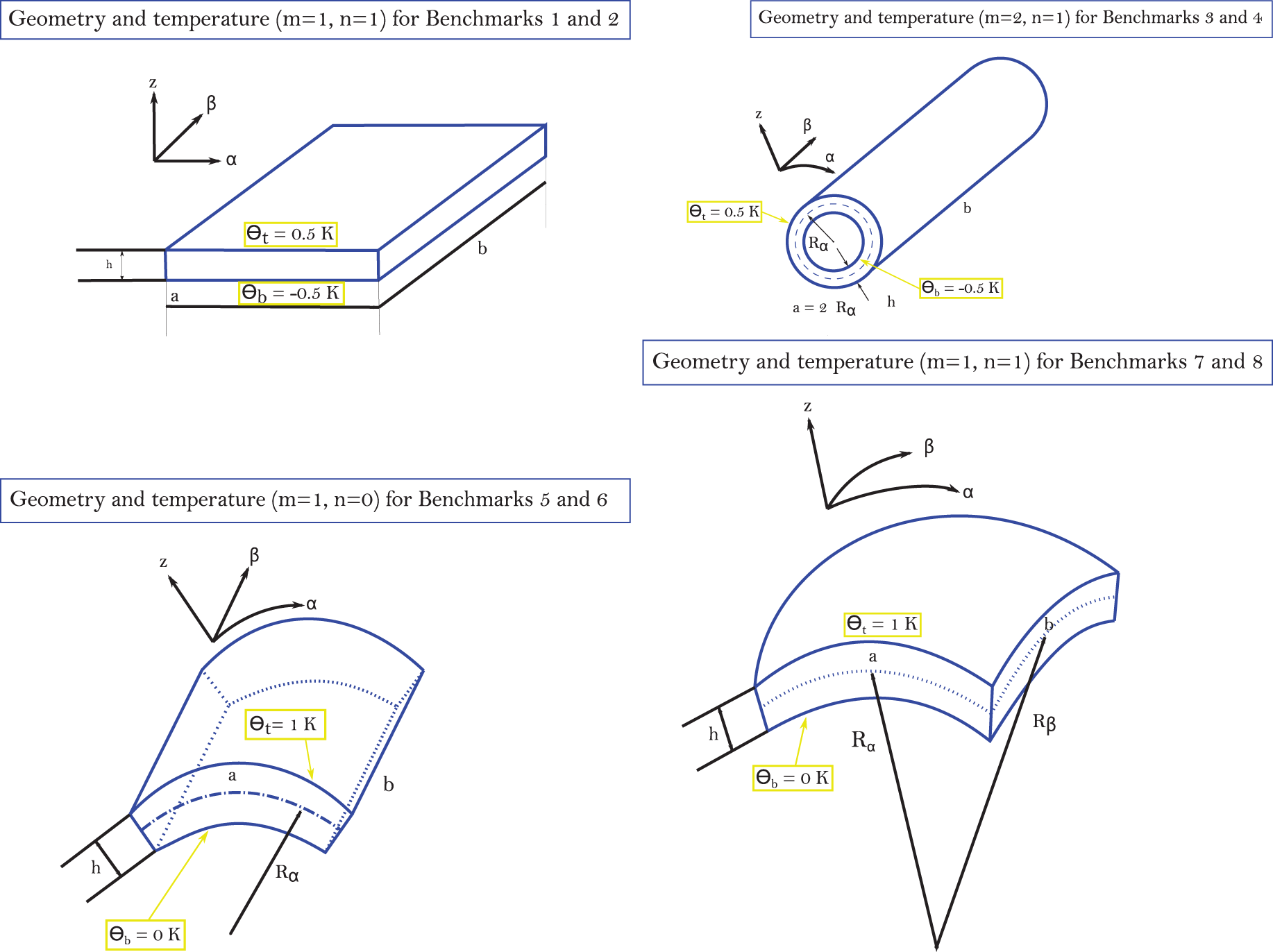
Figure 1: Geometry and applied temperatures for the eight benchmarks
The value h for the thickness is constant in each structure. The origin of these curved coordinates is positioned in an angle, where α and β are parallel to the sideways and located on the centre reference surface Ω0. The middle surface Ω0 is the reference surface for the evaluation of all the geometrical parameters. z is the coordinate in the thickness direction and it is perpendicular to Ω0 and directed towards the top surface. Rα and Rβ are the radii of curvature in the in-plane directions α and β, respectively, and they are considered as constant. a and b are the shell dimensions in α and β directions, respectively. A specific parametric coefficient is calculated for
For shells with constant curvature radii, the parameters
Eqs. (2)–(5) are valid for all the structures proposed in Fig. 1. The relations are proposed for spherical panels having constant radii of curvature because they are the most general. They allow the formulation for plates, cylinders and cylindrical panels by assuming appropriate values for the two radii of curvatures. Eq. (5) is the 3D Fourier heat conduction equation in steady-state conditions specifically written for spherical shells and already presented by Brischetto et al. in [21]. In a full coupled thermoelastic problem, the three-dimensional Fourier heat conduction relation is directly coupled with the three-dimensional equilibrium relations. The three conduction coefficients in the
where the dependence by z is due to
2.2 Geometrical and Constitutive Equations
The geometries proposed are loaded by means of a sovratemperature field
where [ɛααk ɛββk ɛzzk γβzk γαzk γαβk]T are the six components of the strain vector for each k layer and they are defined as the algebraic sum of displacement strain and thermal strain components. The strain components are defined via the vector of displacements
The constitutive equation allows the six strain components to be linked with the six stress components via the elastic coefficient matrix
the stress vector
The analytical form of Eqs. (2)–(5) is only developed for angles of orthotropy
The closed-form solution of the coupled relations (2)–(5) is defined via the imposition of the harmonic form for displacement components and sovra-temperature. This feature means simply supported boundary conditions for all the analyses that will be carried out. The harmonic relations for displacement components and the temperature field are:
where the two parameters
The introduction of the harmonic expression of the displacements and temperature profile (Eqs. (13)–(15)), the geometrical relations and the constitutive equations (Eqs. (7)–(12)) into the coupled thermo-mechanical Eqs. (2)–(5) gives a set of four differential relations written as functions of maximum values for the displacement components and for the sovra-temperature with associated derivatives defined in z. The derivatives performed in
This system of equations can be decreased to a first order one via the methodology discussed in [66] and [67]. The order of the derivatives performed in z is decreased when the number of unknowns in all j layers is redoubled from 4 (
Eq. (20) can be compacted as:
where
with
A general homogeneous system of first order differential relations can be proposed as:
In analogy, the resolution of Eq. (23) becomes:
Eq. (26) is employed to define the unknown vector
where
an alternative form of Eq. (28) is:
where
Eq. (29) connects the top and bottom unknown vector (primary variables and the related derivatives in
The requirements specified in Eq. (30) are obviously imposed for the displacement maximum values
In Eqs. (30) and (31), for each considered unknown, the continuity is established between the evaluation made at the lowest point (b) of the general j-th layer and the evaluation made at the highest point (t) of the (
The diagonal part composed of 1 indicates the congruence conditions expressed as displacement components and the continuity of temperature written in Eq. (30). The other coefficients
Eq. (33) allows linking unknows and related derivatives in z defined at the bottom of the j layer with unknows (and related derivatives in
All structures taken into account have simply supported sides, this boundary condition is automatically imposed via the harmonic forms for all the primary unknowns:
In addition, load boundary requirements must be imposed at the top and bottom of the structures. These conditions can be written as:
the last equations allow to impose the sovra-temperature values directly at the top and bottom of the structure for the pure thermal stress analysis. Eq. (36) can be rewritten, in matrix form as:
Eqs. (37) and (38) can be compacted as:
subscripts t and b indicate the highest and lowest point, respectively. Superscript M shows the last artificial layer and superscript 1 shows the first artificial layer. Vector
In order to include Eqs. (39) and (40) into a matrix expression of an algebraic system, it is useful to indicate
Eq. (41) defines the
Using Eqs. (42), (39) can be rewritten in terms of
Eqs. (43) and (40) can be now compacted as:
where
and
Matrix
After the calculation of the displacements at the bottom, Eqs. (33) and (29) can be subsequently employed to define the displacement components and temperature (and connected derivatives made with respect to
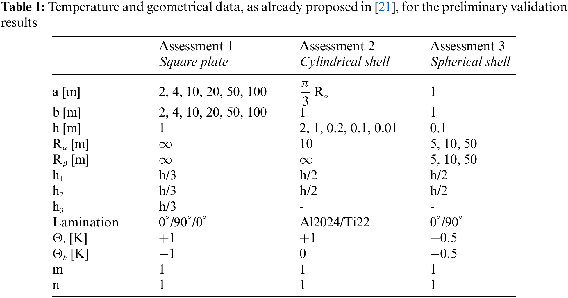
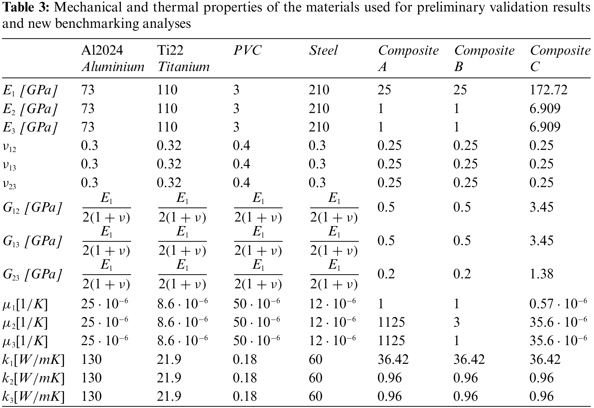
The first part of this section shows three preliminary validation results to verify the developed general three-dimensional exact coupled thermo-elastic shell theory. Comparisons with [21] are performed to define the appropriate order of expansion N for the exponential matrix in Eq. (27) and the correct number of artificial layers M for the exact definition of constant curvature terms related to shell geometry. After the authentication of the model, new benchmarking analyses are proposed in the second part of this section. N and M parameters are opportunely chosen and the new results discuss the effects of thickness ratios, structure geometries, lamination sequences, embedded materials and sovra-temperature impositions when a 3D thermal stress investigation of shells and plates is performed. All the geometrical data for the validation results and benchmarks proposed in this section are available in Tables 1 and 2, material data are shown in Table 3. In Table 3,
Tables 4–14 present four different acronyms used to indicate the different models compared in this section: 3D-u-
3.1 Preliminary Validation Results
A number of three preliminary validation results are employed for the validation of this new three-dimensional general exact coupled thermo-elastic shell model, indicated as 3D-u-
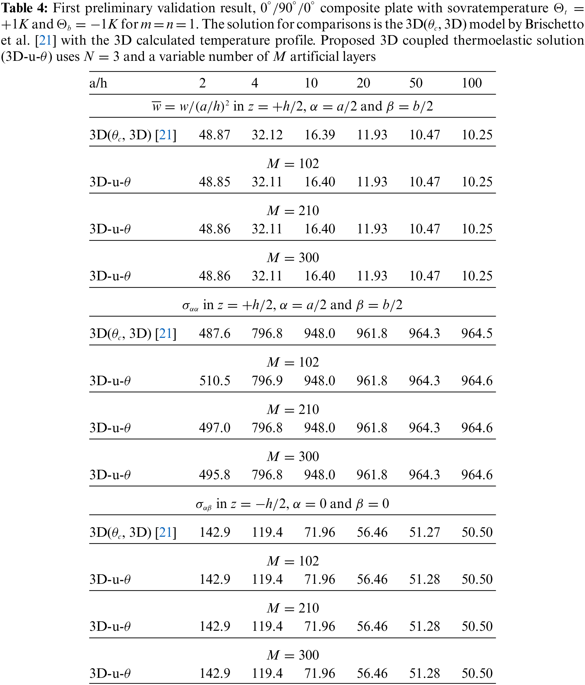
The first preliminary validation result considers a square plate having simply-supported sides. The geometrical data can be seen in the second column of Table 1 and the material data can be seen in Table 3, in correspondence to the Composite A column. The results considered as a reference are those obtained via the 3D(
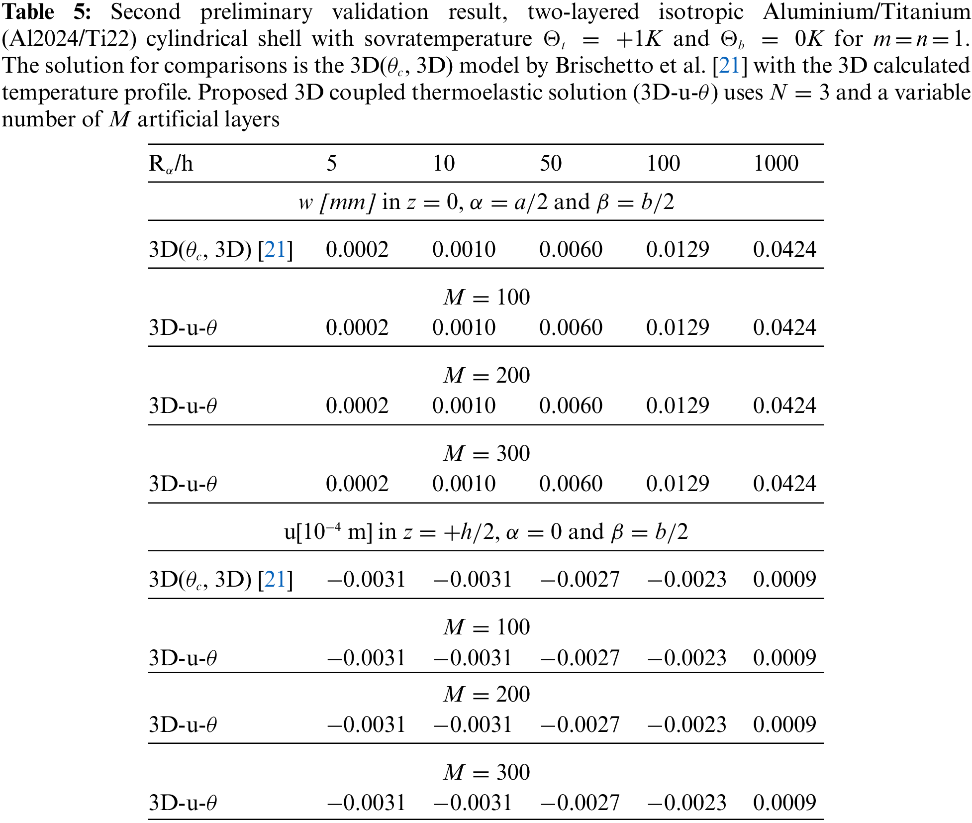
The second preliminary validation result shows a two-layered isotropic cylindrical shell having simply-supported sides. The geometrical data can be seen in the third row of Table 1 and the material data can be seen in Table 3, in correspondence to the Aluminium column (for the bottom physical layer) and the Titanium column (for the top physical layer). The two physical layers have completely different thermal and elastic properties. The employed reference results come from the 3D(
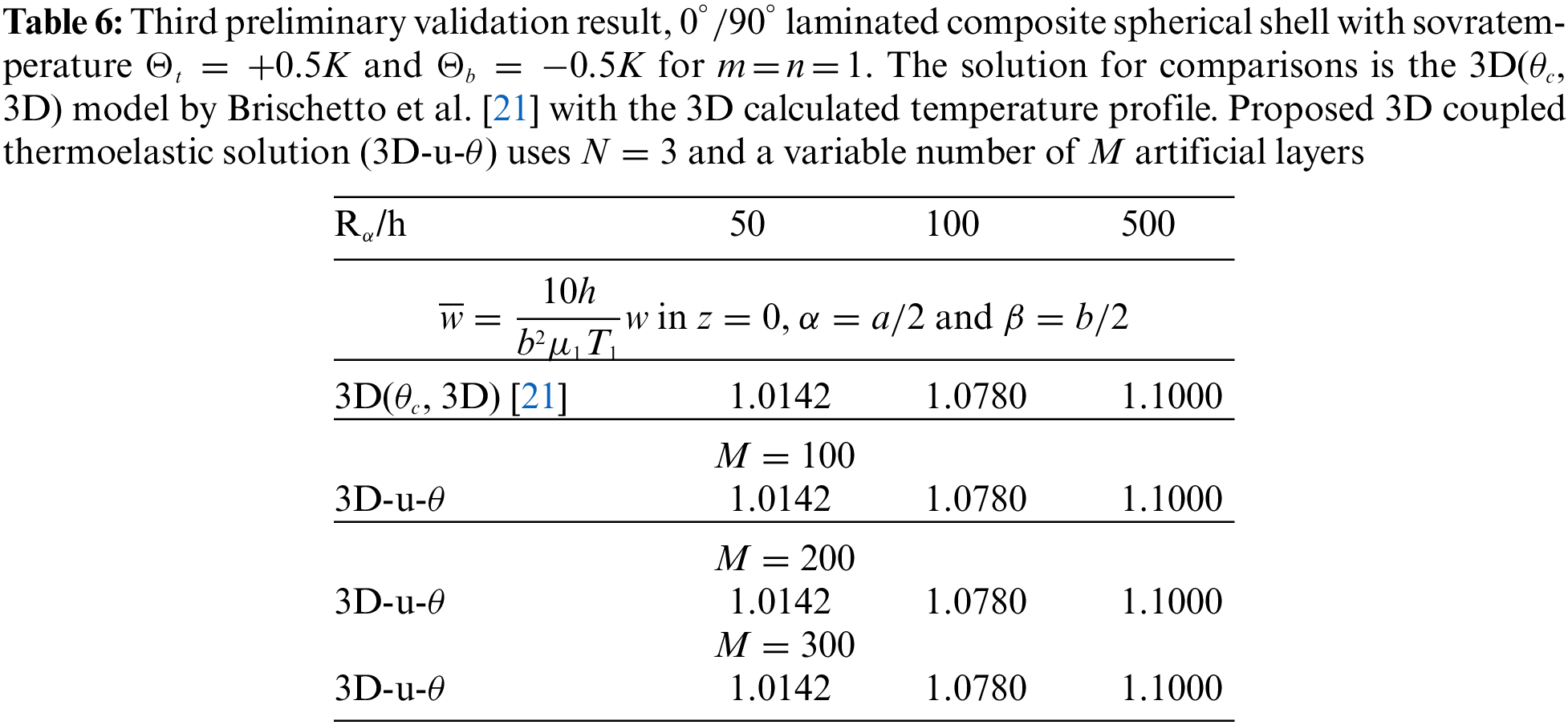
The last and third preliminary validation result proposes a simply-supported spherical shell. The configuration and the geometrical data can be visualized in Table 1. The material used for this validation result is the Composite B material shown in Table 3. The non-dimensional transverse displacement is written as
The next section proposes new benchmarking analyses where different geometrical data, thickness ratios, lamination stacking sequences, materials, temperature profiles and displacement-stress studies are proposed. Even if the preliminary results suggest
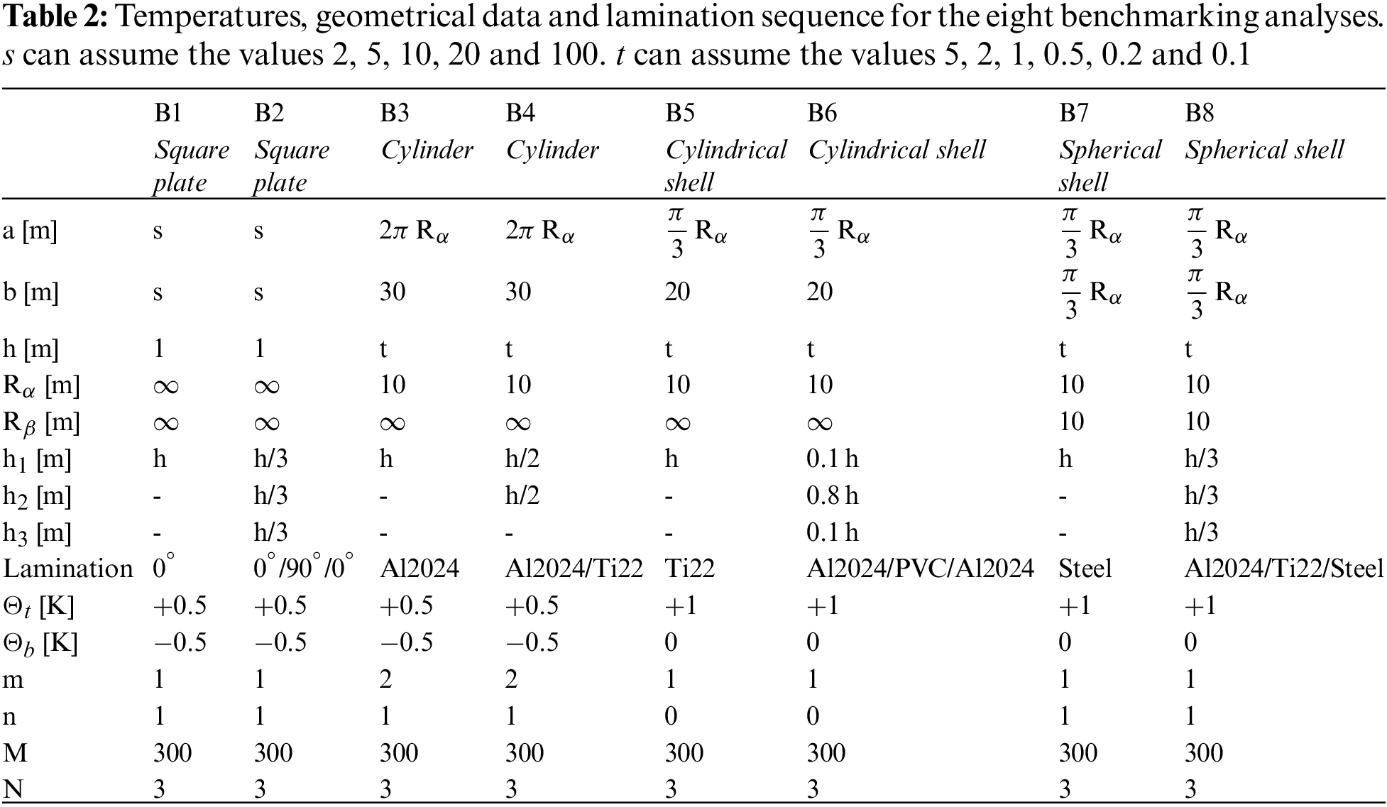
Eight benchmarking analyses are here discussed for cylindrical and spherical panels, cylinders and plates. Temperature is enforced at the outer faces with different amplitudes and half-wave numbers (see Fig. 1 for further information about geometrical data and temperature applications). In these new results, several lamination schemes and materials are considered. Therefore, each configuration can be one-layered or/and multi-layered. The 3D-u-
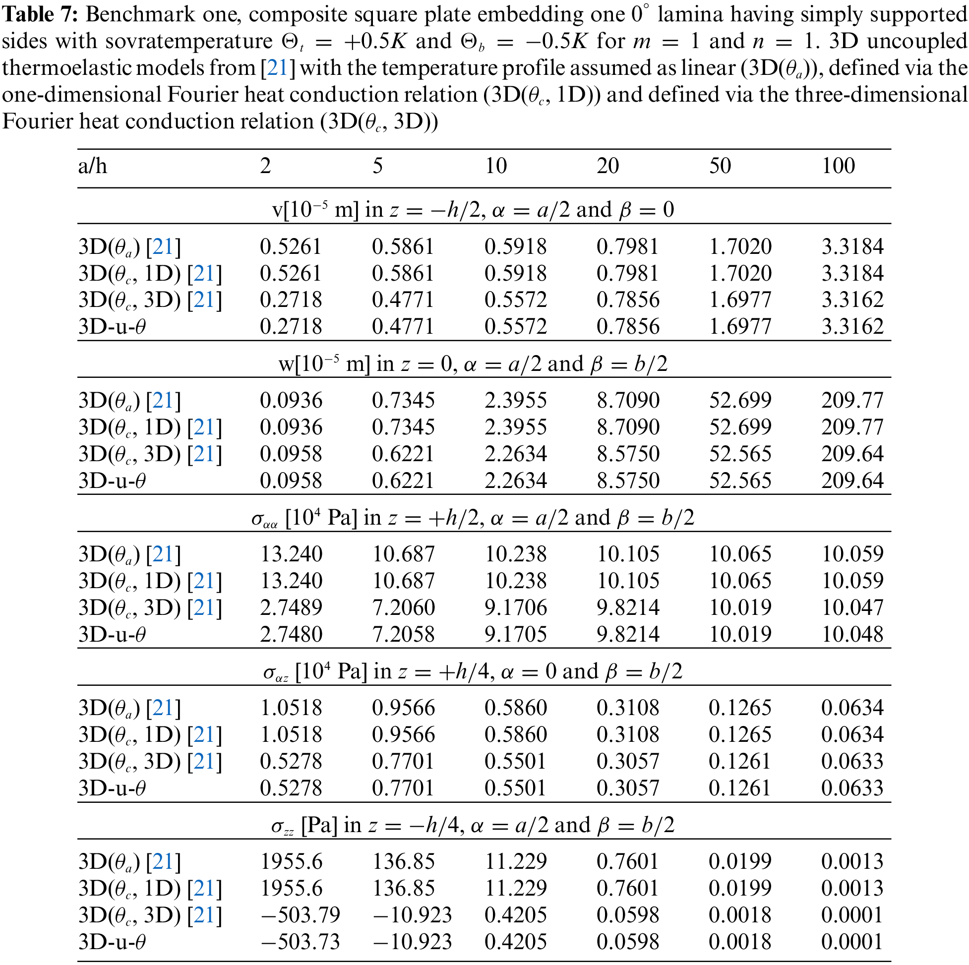
The first benchmark represents a square one-layered composite plate with simply-supported sides (see Fig. 1). The geometrical and material data used for this case are written in Table 2 (column B1) and in Table 3 (the material used is Composite C). The considered thickness ratios are highlighted in Table 2. Fig. 2 gives the temperature evaluation in the thickness direction of a thick and a thin plate. In the thin one-layered composite plate, all the temperature profiles (calculated via (
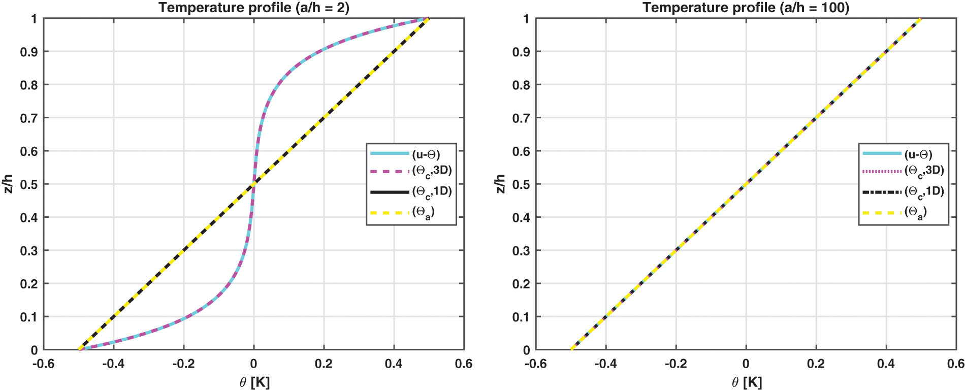
Figure 2: Benchmark one, temperature profiles for two different
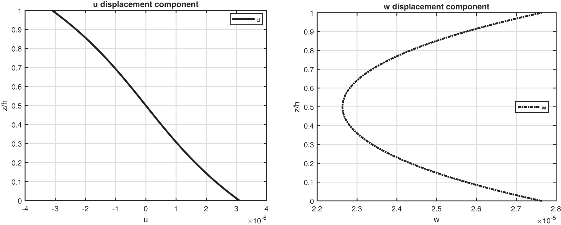
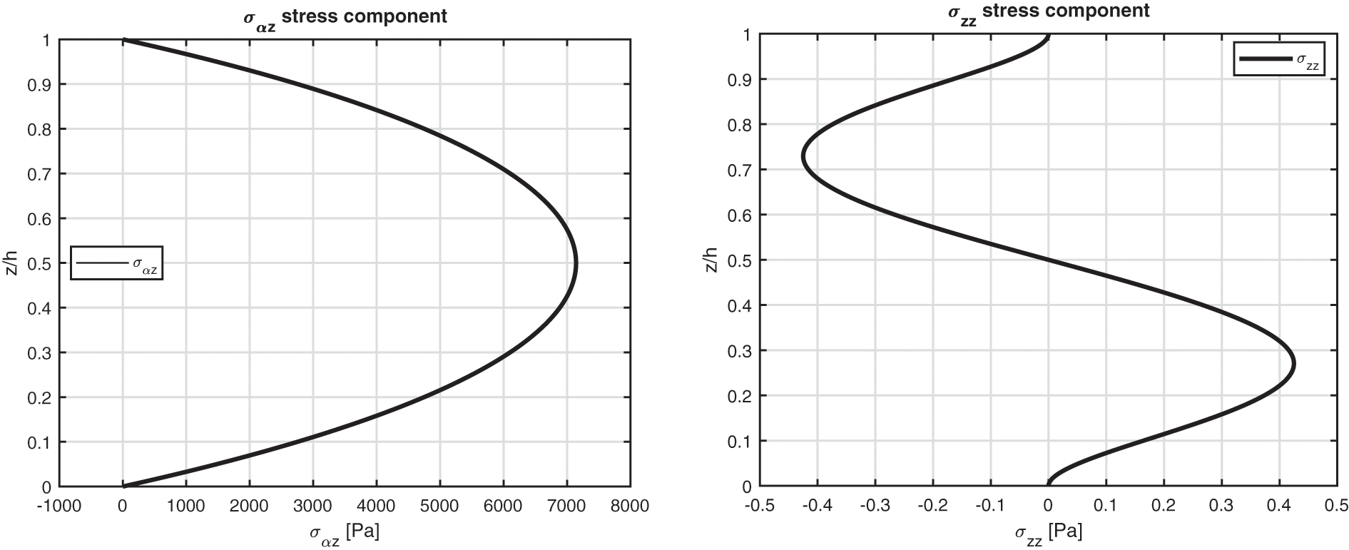
Figure 3: Benchmark one, displacement components and stress components for a moderately thick composite square plate embedding one
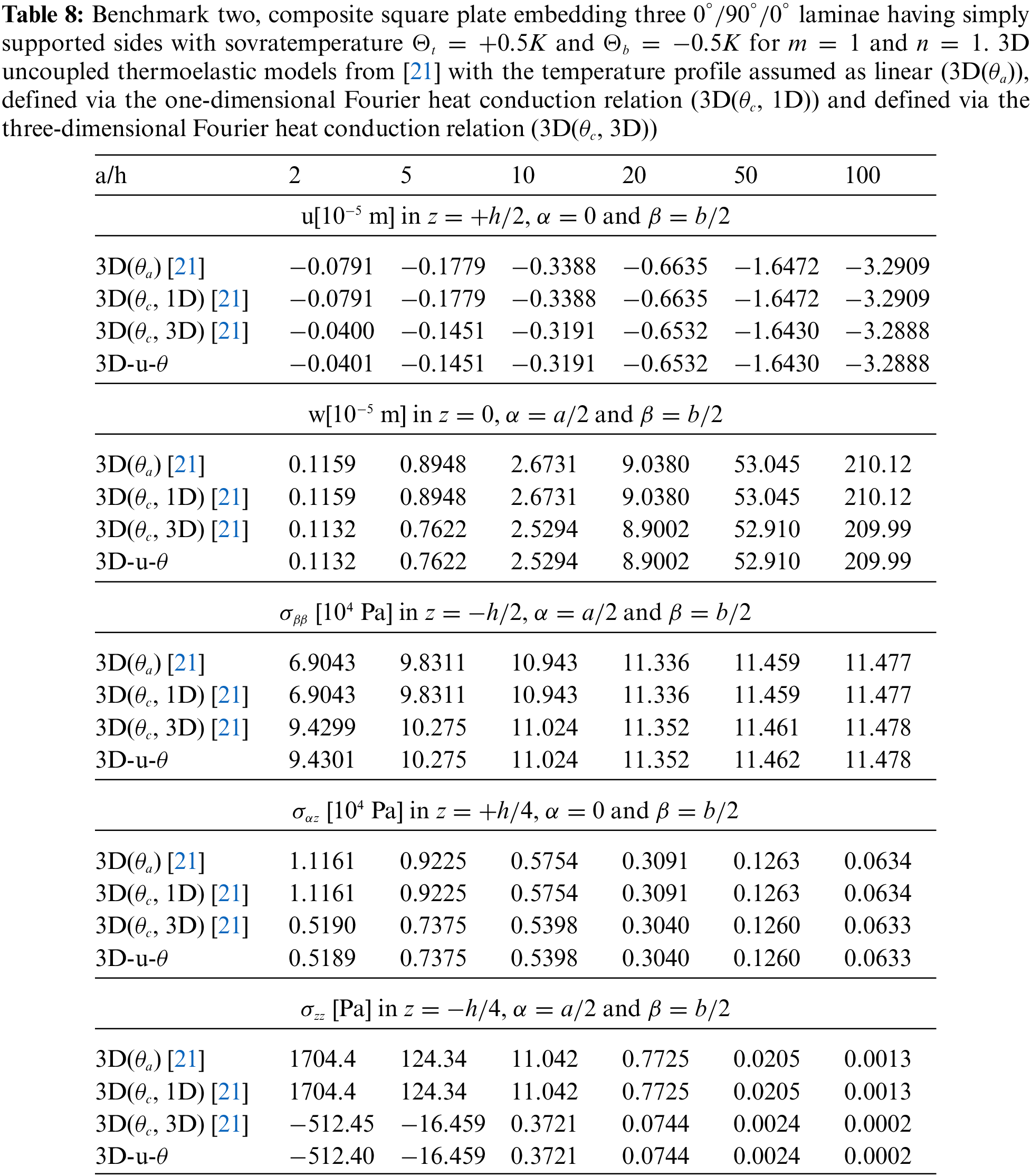
The second benchmark shows a square composite plate, equally divided in three layers, having simply-supported sides (in Fig. 1 the structure is shown). Geometrical data are available in Table 2 and material data are available in the column Composite C of Table 3. The sovra-temperature profiles in the thickness direction shown in Fig. 4 do not change with respect to the previous benchmark because the two sides have the same value (
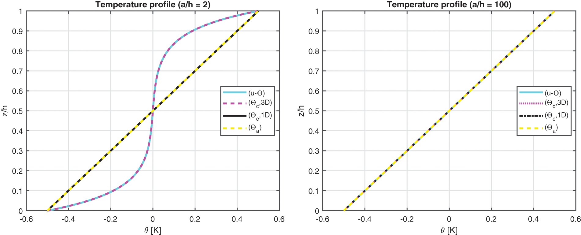
Figure 4: Benchmark two, temperature profiles for two different
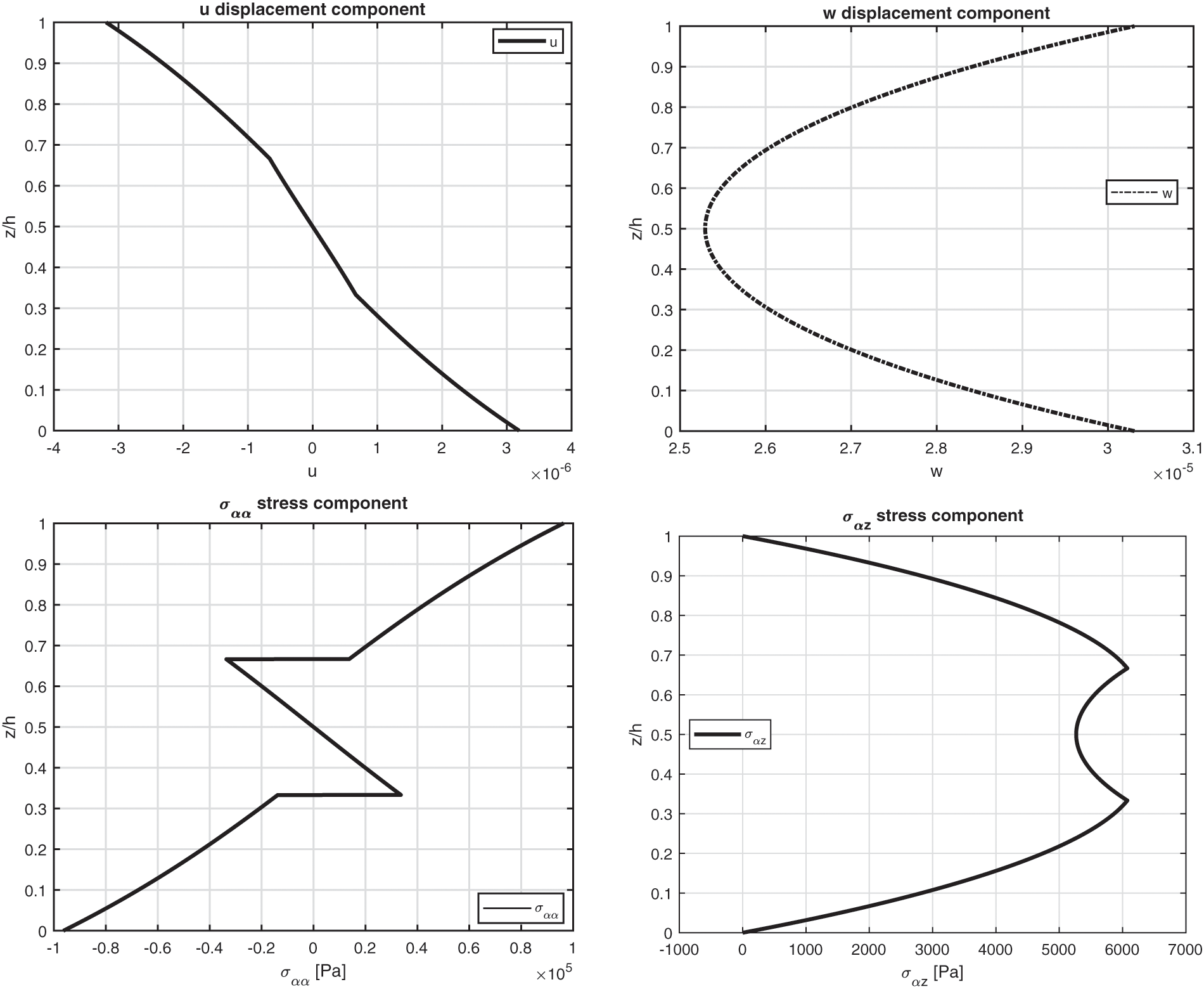
Figure 5: Benchmark two, displacement components and stress components for a moderately thick composite square plate embedding three
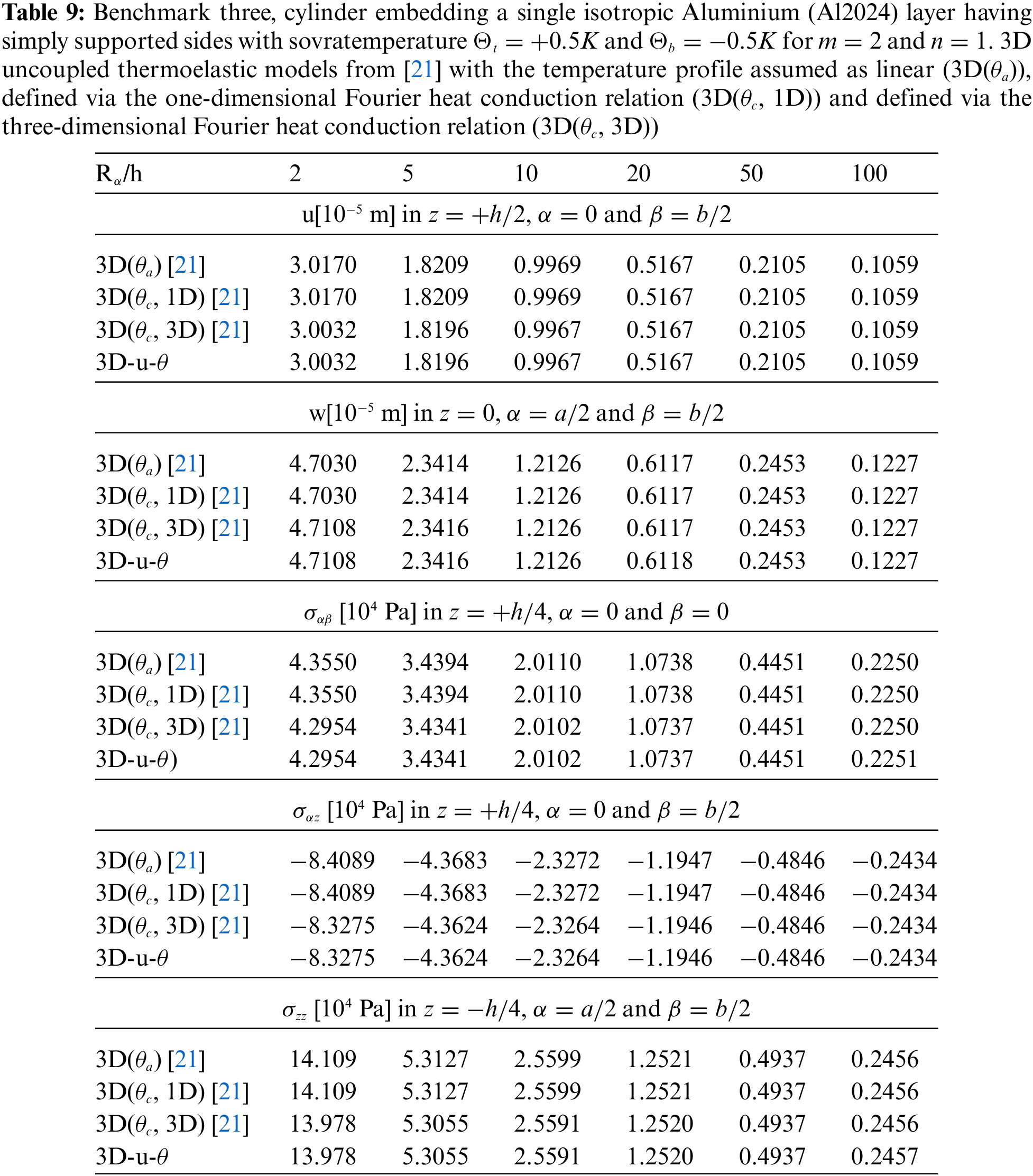
The third benchmark shows an isotropic homogeneous cylinder having simply supported sides (see Fig. 1). All the characteristics are written in Table 2, for what concerns the geometrical data, and in Table 3, for what concerns the material employed (Aluminium Al2024). The temperature profiles are shown in Fig. 6 for a thick and a thin structure. In this benchmark, the effect connected with the thickness layer for thick cylinders is negligible due to the symmetry and the rigidity of the geometry. These conclusions are still valid for the displacement and stress components discussed in Table 9; here, 3D(
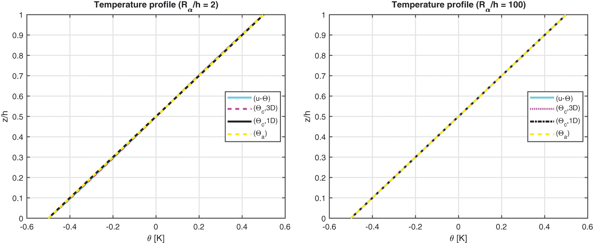
Figure 6: Benchmark three, temperature profiles for two different
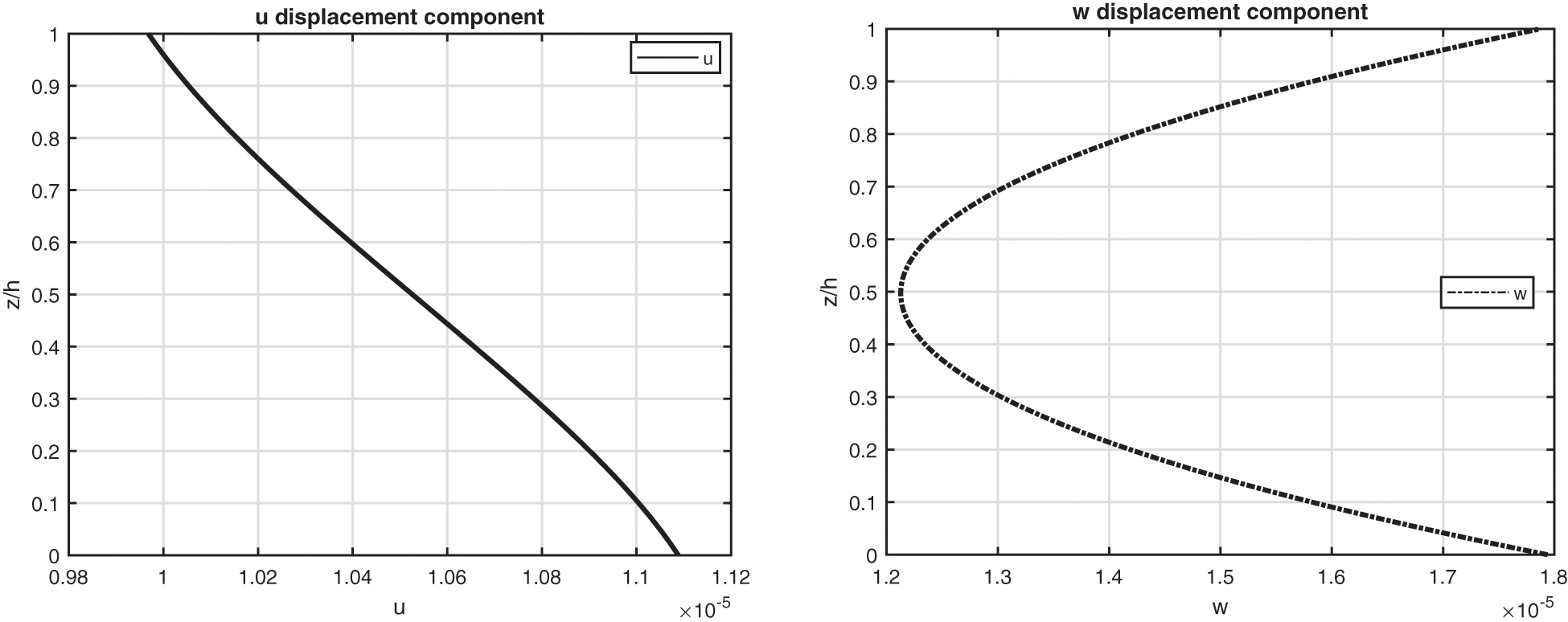
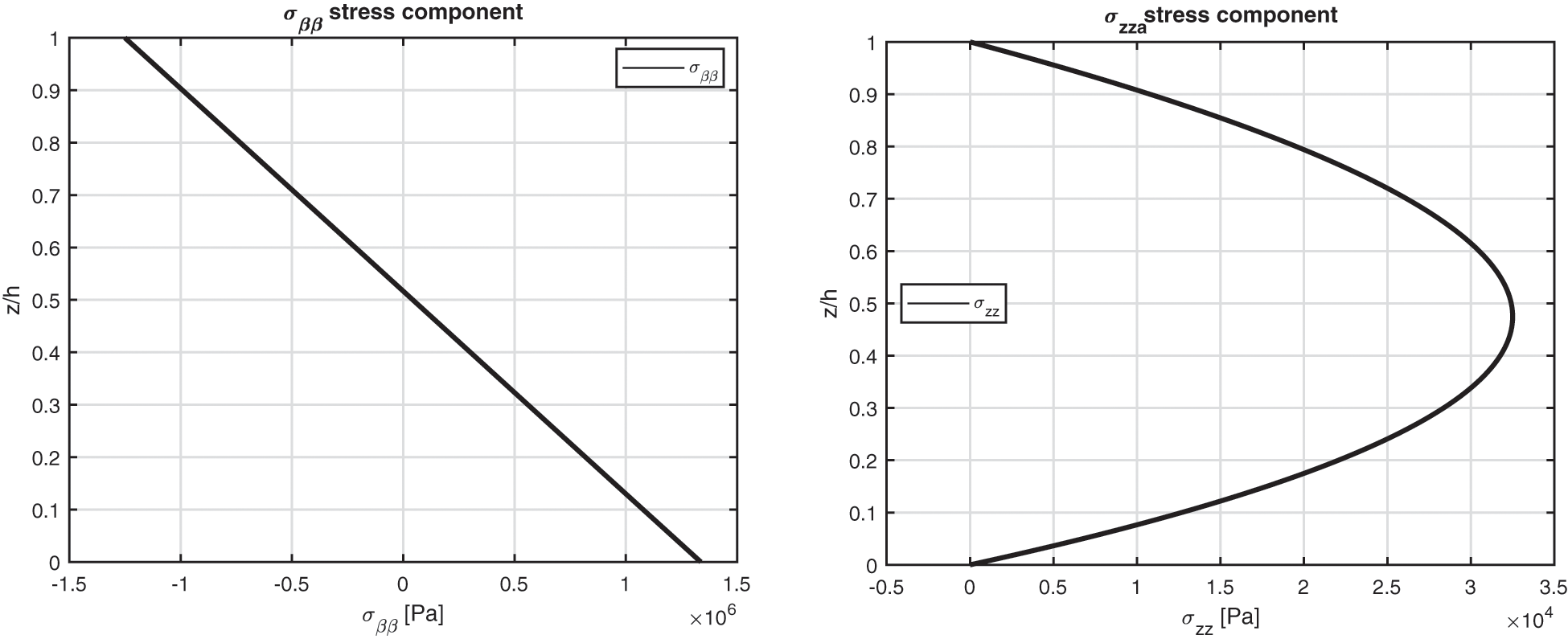
Figure 7: Benchmark three, displacement components and stress components for a moderately thick cylinder embedding a single isotropic Aluminium (Al2024) layer (
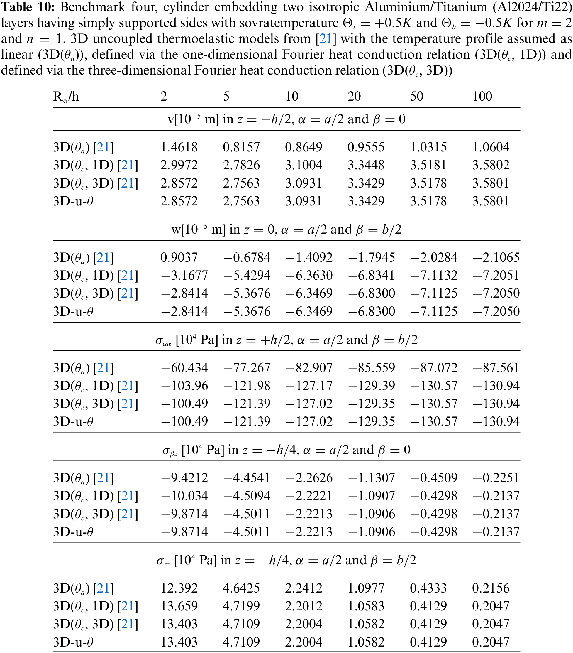
The benchmark number four discusses an isotropic two-layered cylinder with simply supported sides (see Fig. 1 to visualize the case). Geometrical data are available in Table 2 in the column B4 and the mechanical properties of the material are written in Table 3 (for the bottom physical layer the reference column is Aluminium, for the top the reference column is Titanium). The results in Fig. 8 demonstrate that the temperature evaluation is never linear even when the cylinder is thin (except for the (
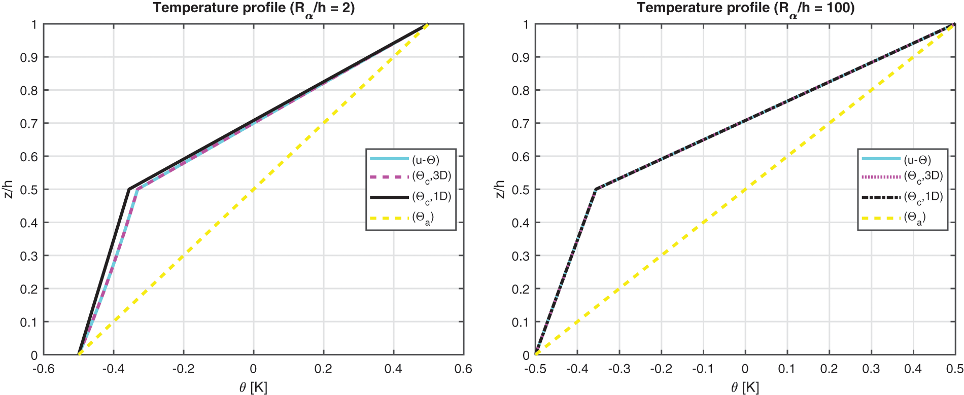
Figure 8: Benchmark four, temperature profiles for two different
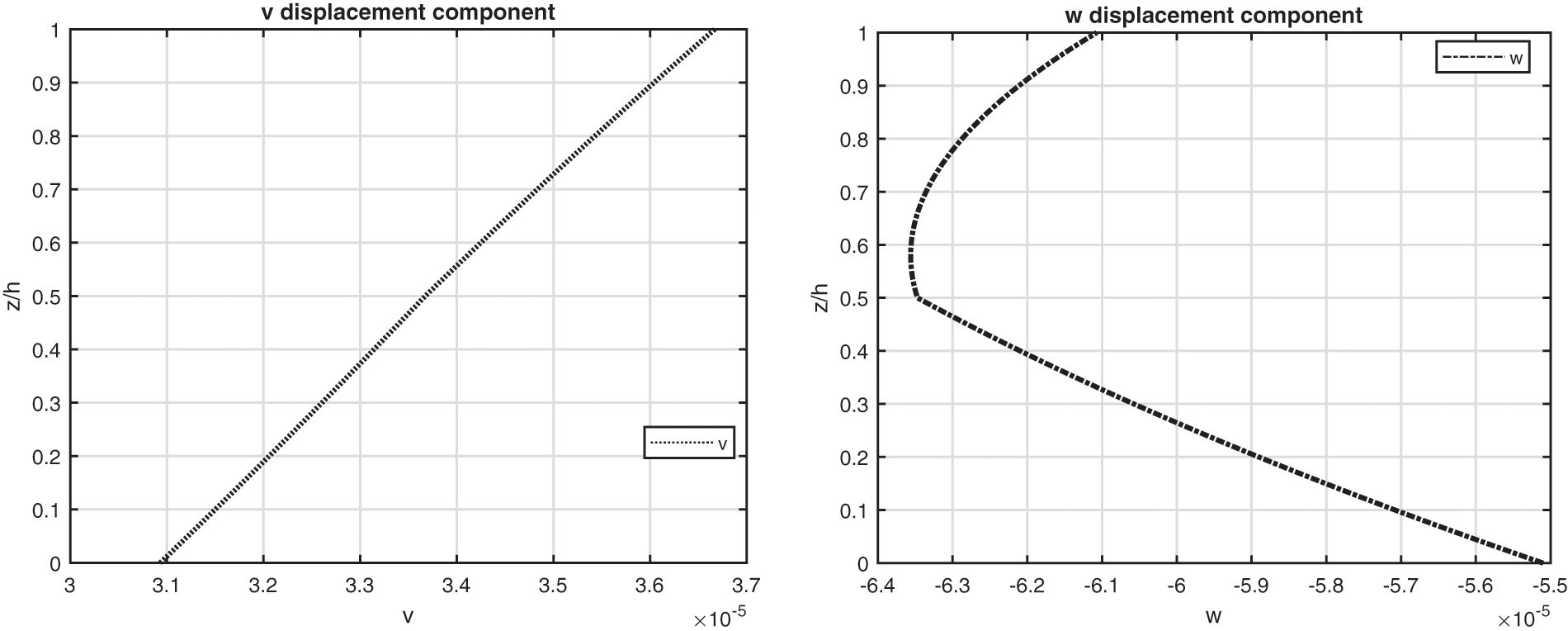
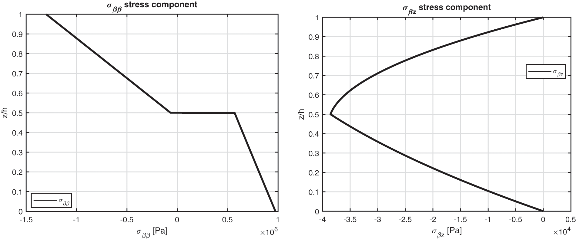
Figure 9: Benchmark four, displacement components and stress components for a moderately thick cylinder embedding two isotropic Aluminium/Titanium (Al2024/Ti22) layers (
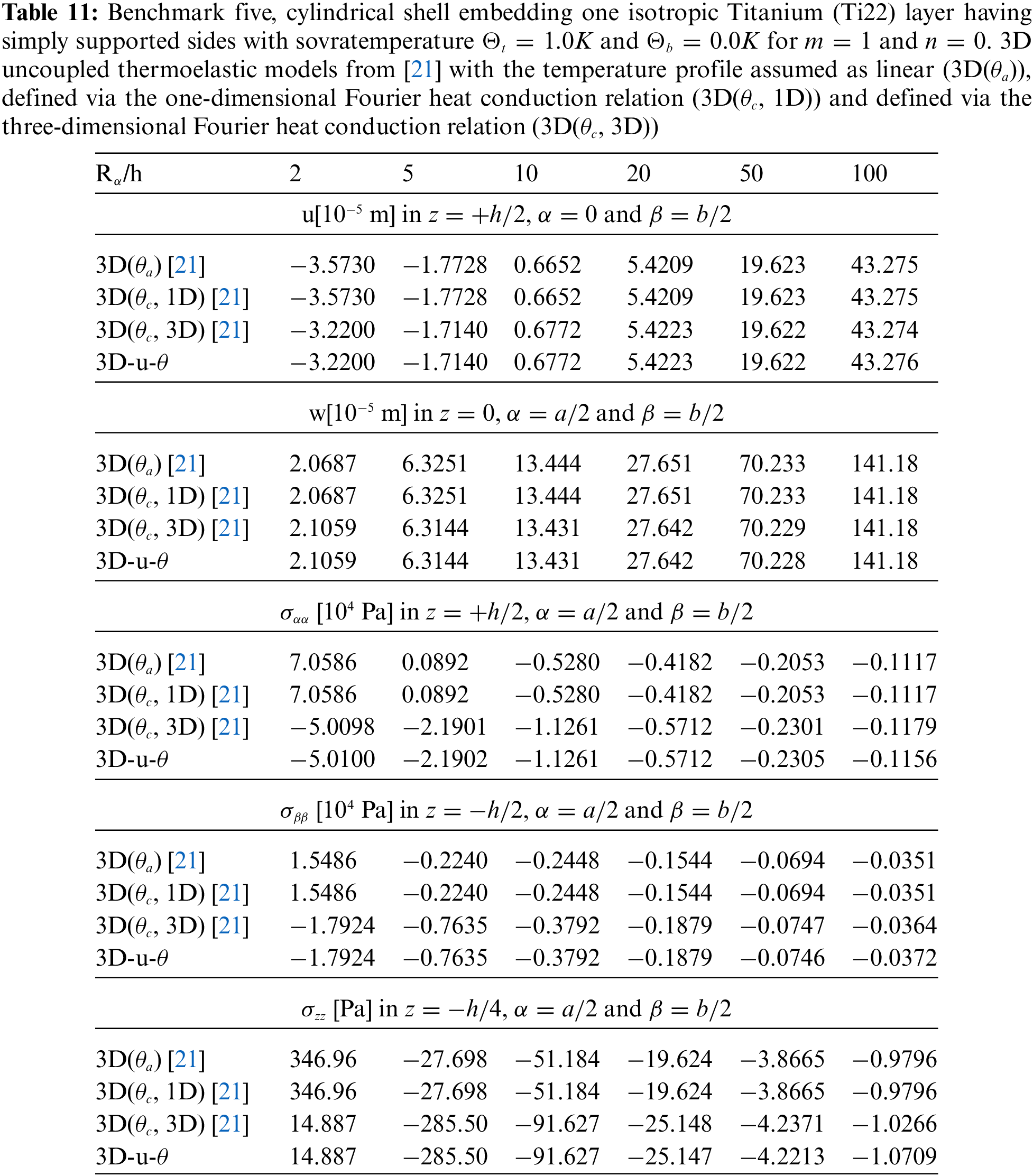
The fifth benchmark analyses an isotropic one-layered cylindrical panel having simply supported sides (see Fig. 1). The mechanical and thermal properties
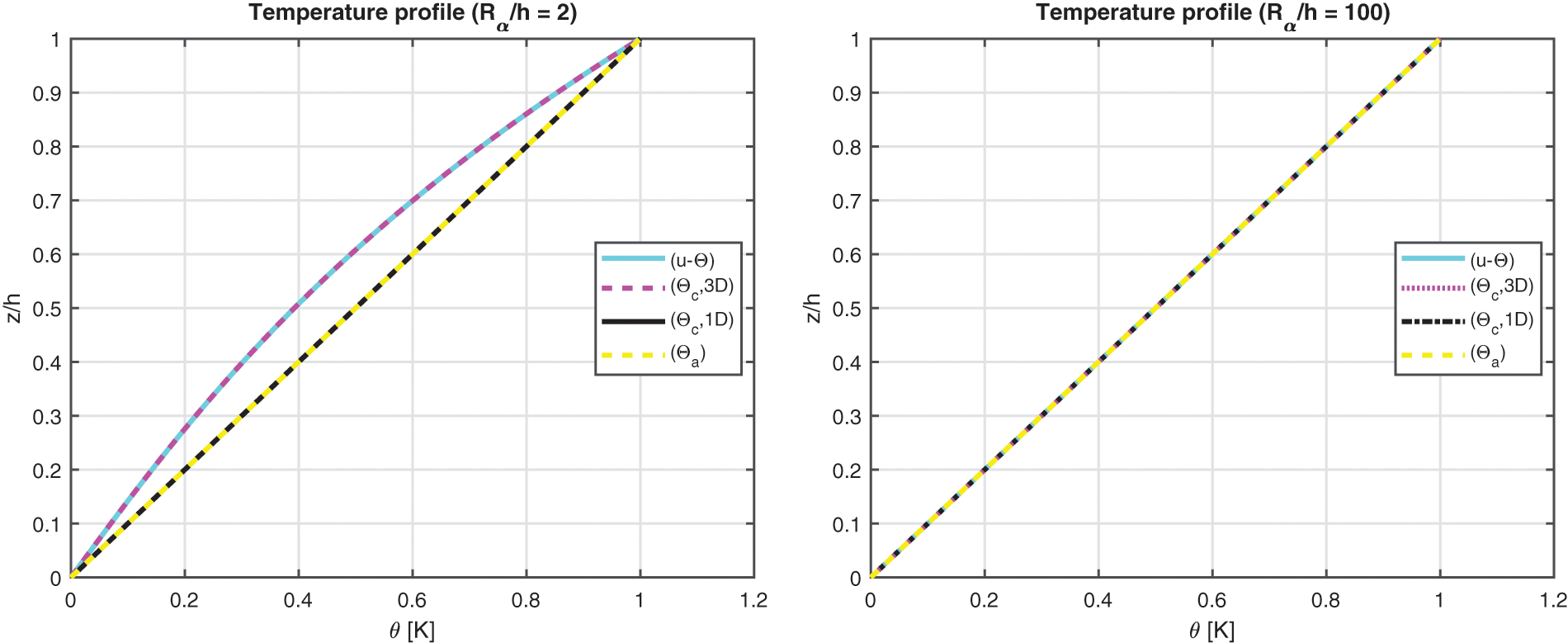
Figure 10: Benchmark five, temperature profiles for two different
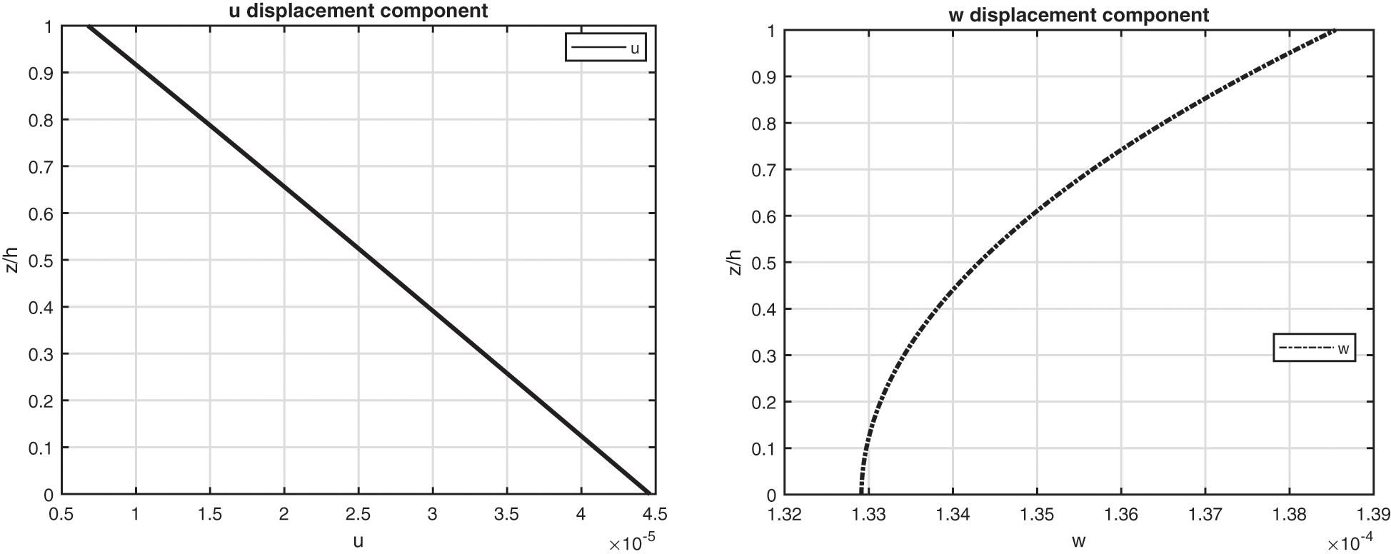
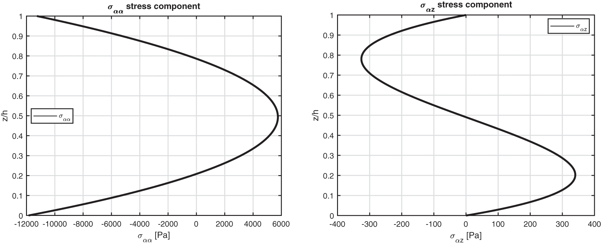
Figure 11: Benchmark five, displacement components and stress components for a moderately thick cylindrical shell embedding one isotropic Titanium (Ti22) layer (
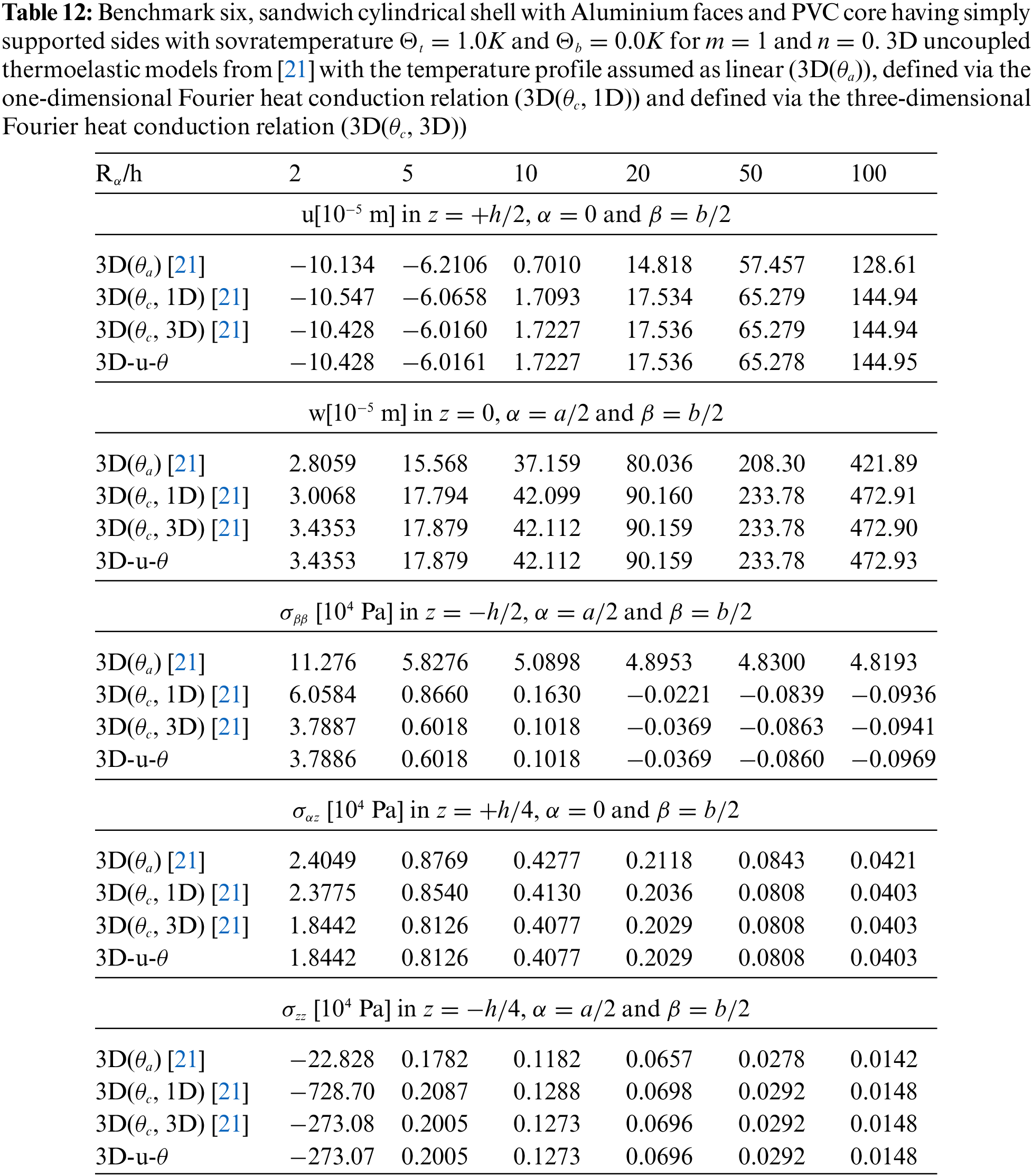
The benchmark number six analyses the thermal stress investigation of a sandwich cylindrical panel (in Fig. 1 is represented the specific geometry). The geometrical data of the case are presented in Table 2. The skins material is made of Aluminium and the core material is PVC (the mechanical properties are written in Table 3, both for skins and core). Results of Fig. 12 show how the calculated temperature behaviour is mandatory for both thick and thin sandwich shells. The sovra-temperature evaluation is always different from the linear behaviour and it has a typical zigzag form because the thermal properties of the faces are different from those of the core. When a thick sandwich panel is considered, the sovra-temperature evaluation obtained from the 3D(
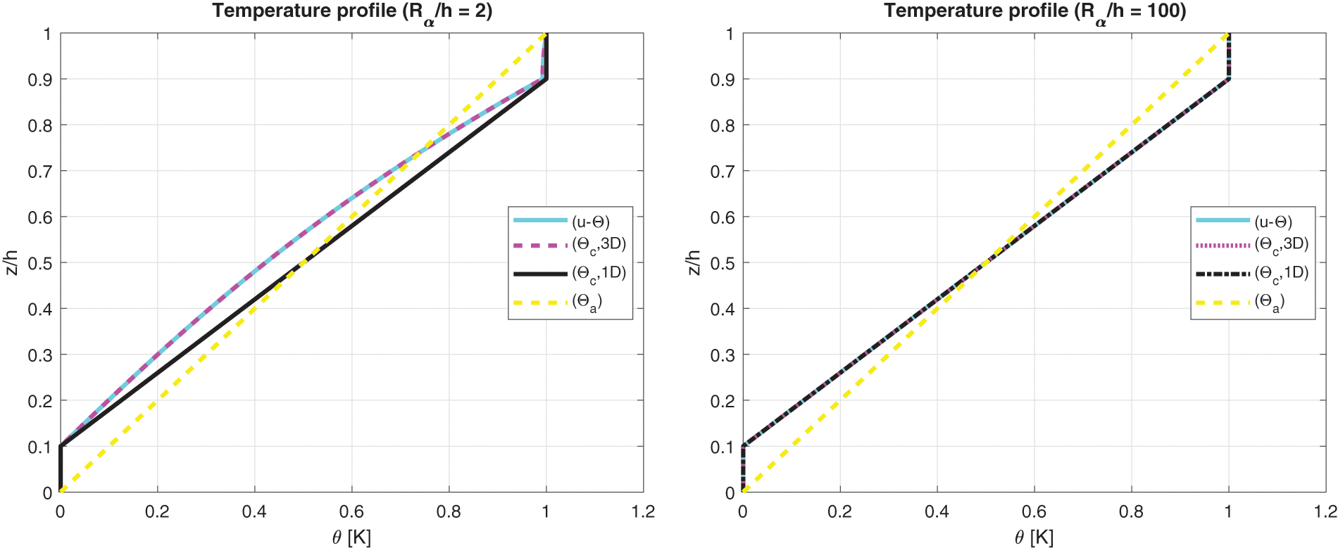
Figure 12: Benchmark six, temperature profiles for two different
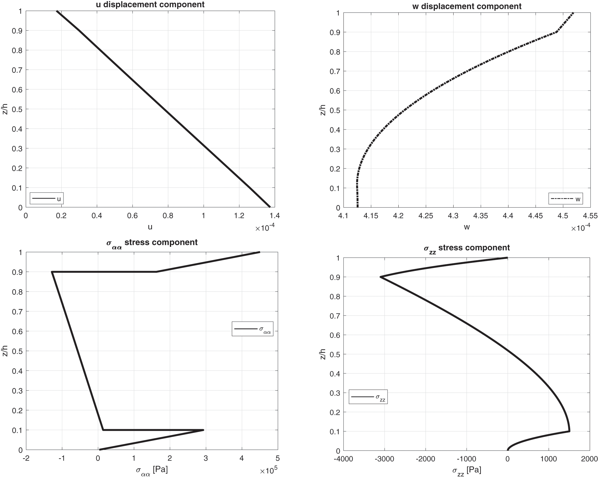
Figure 13: Benchmark six, displacement components and stress components for a moderately thick sandwich cylindrical shell with Aluminium faces and PVC core (
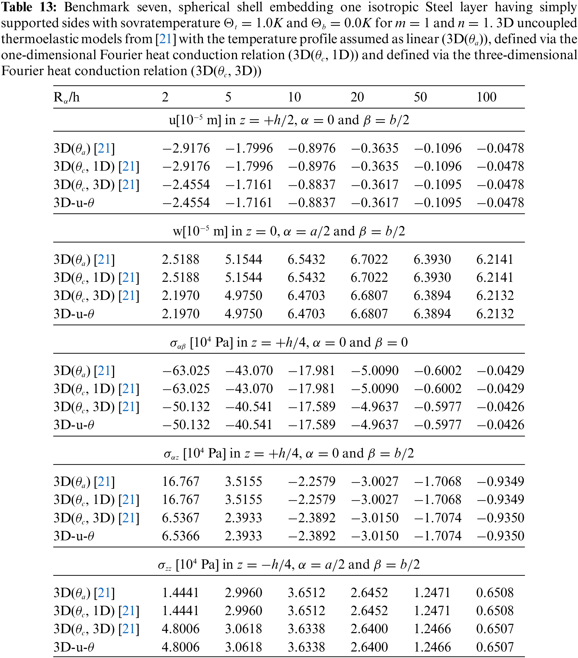
The benchmark seven proposes an isotropic one-layered spherical panel having simply-supported sides (see Fig. 1). Table 2 contains the geometrical data and the column Steel of Table 3 contains the mechanical and thermal properties. Sovra-temperature profiles in Fig. 14 demonstrate how their behaviours are linear in the thickness direction for a thin structure. The temperature has to be defined via the 3D-u-
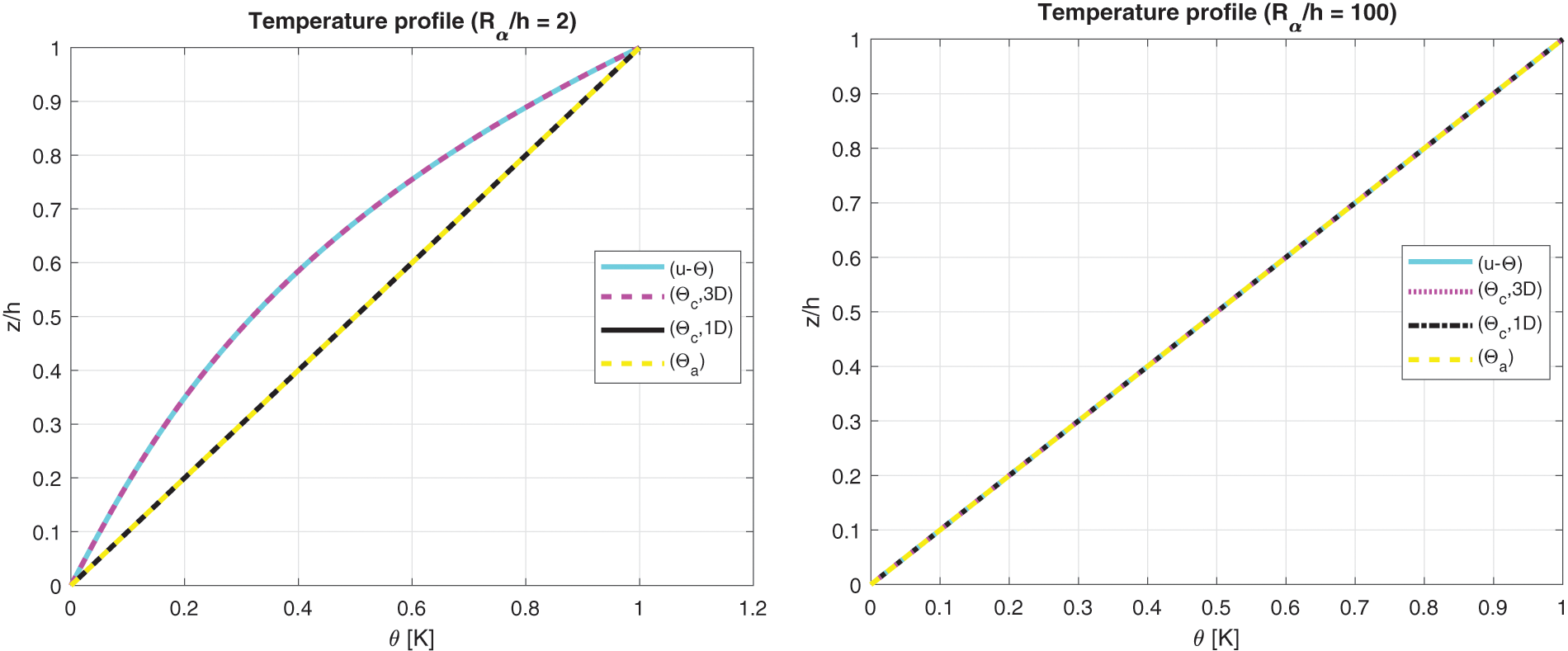
Figure 14: Benchmark seven, temperature profiles for two different
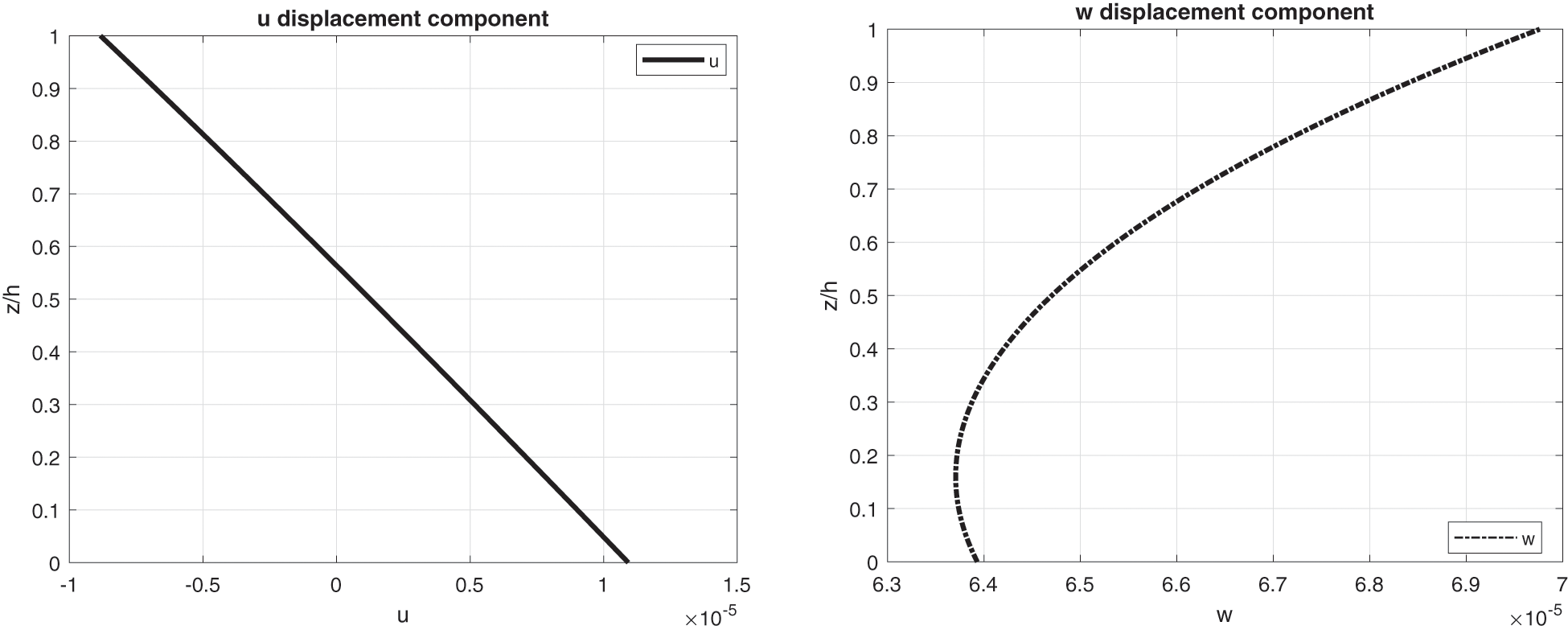
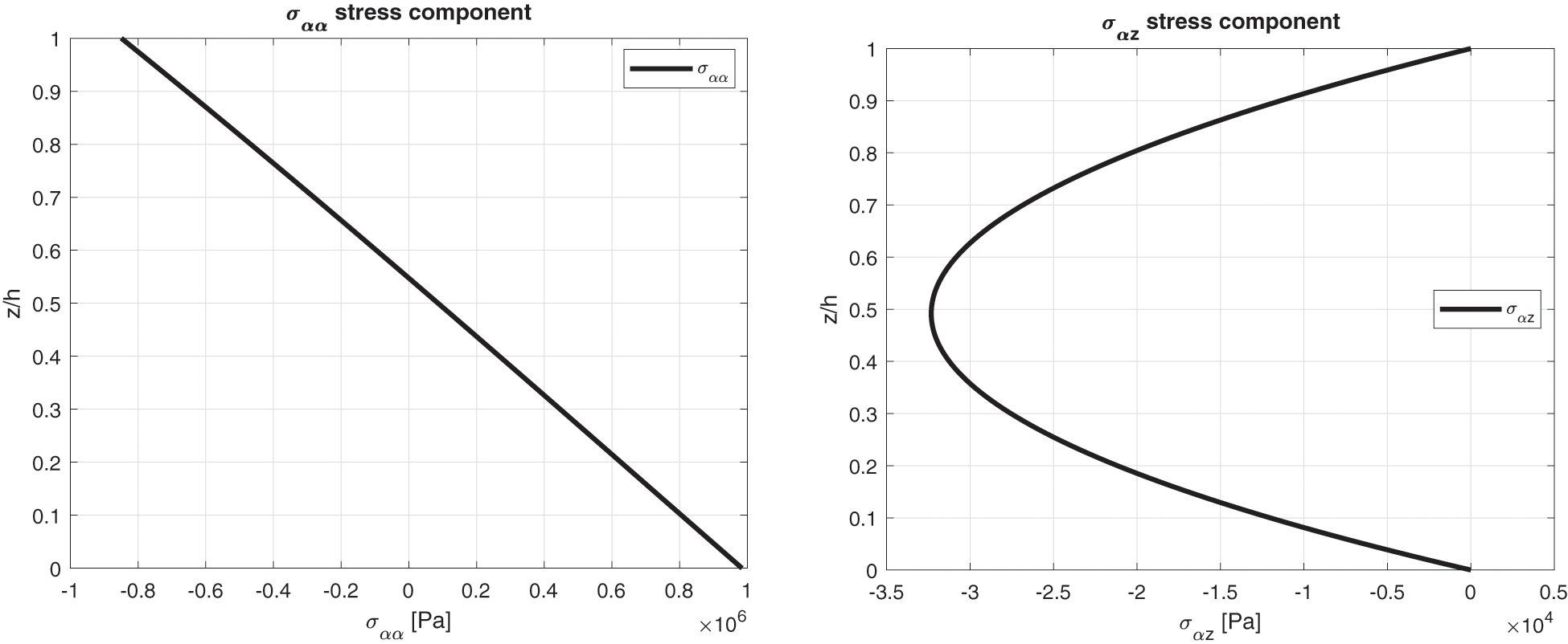
Figure 15: Benchmark seven, displacement components and stress components for a moderately thick spherical shell embedding one isotropic Steel layer (
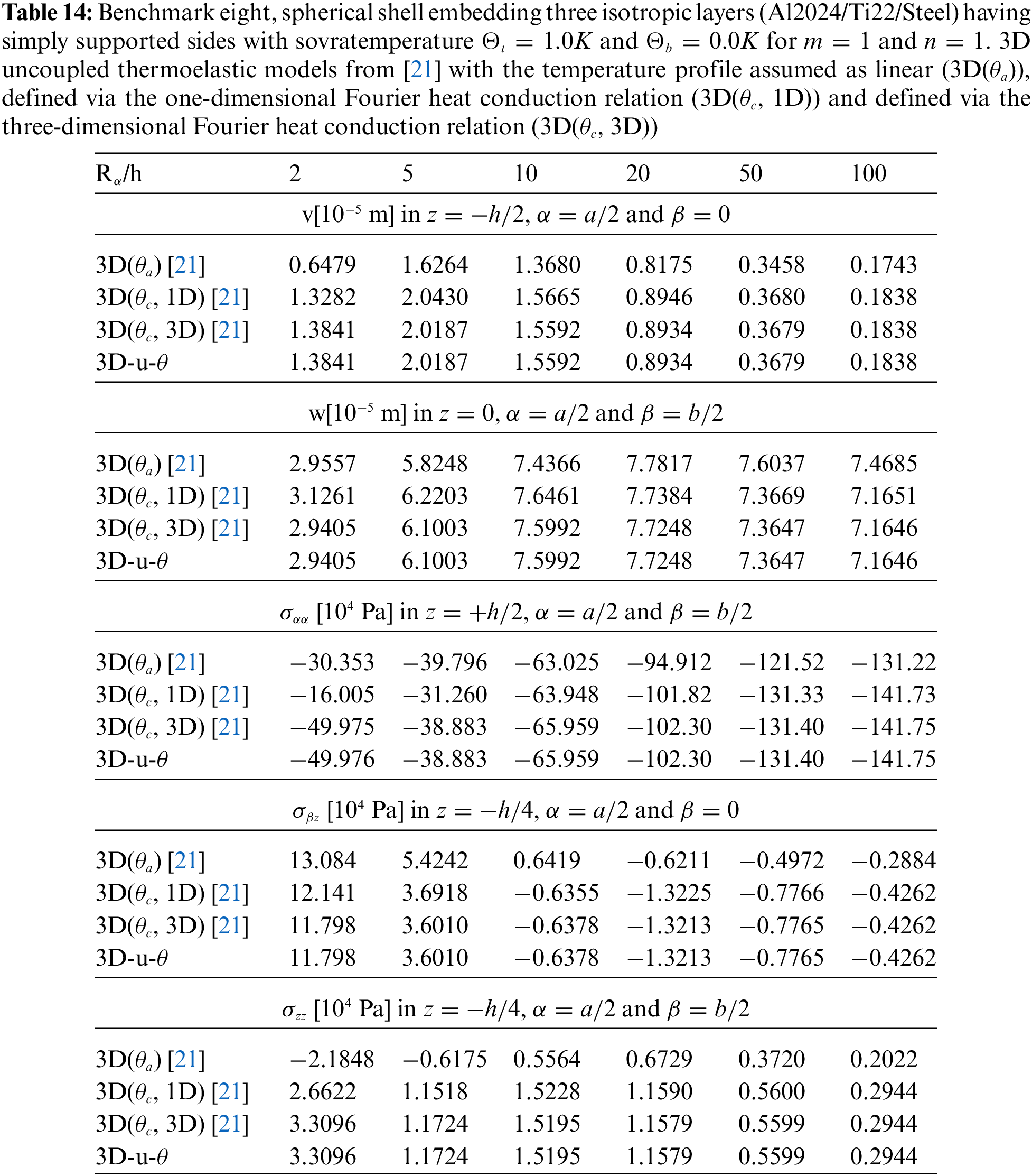
The last and eighth benchmark shows an isotropic three-layered spherical panel having simply-supported sides (consult Fig. 1 to visualize the structure). The geometrical characteristics are contained in Table 2 and the properties for the three used materials are written in Table 3: Aluminium, Titanium and Steel (from bottom to top of the structure). The global thickness h is equally divided in three portions. Fig. 16 confirms that the temperature profile has to be calculated with 3D-u-
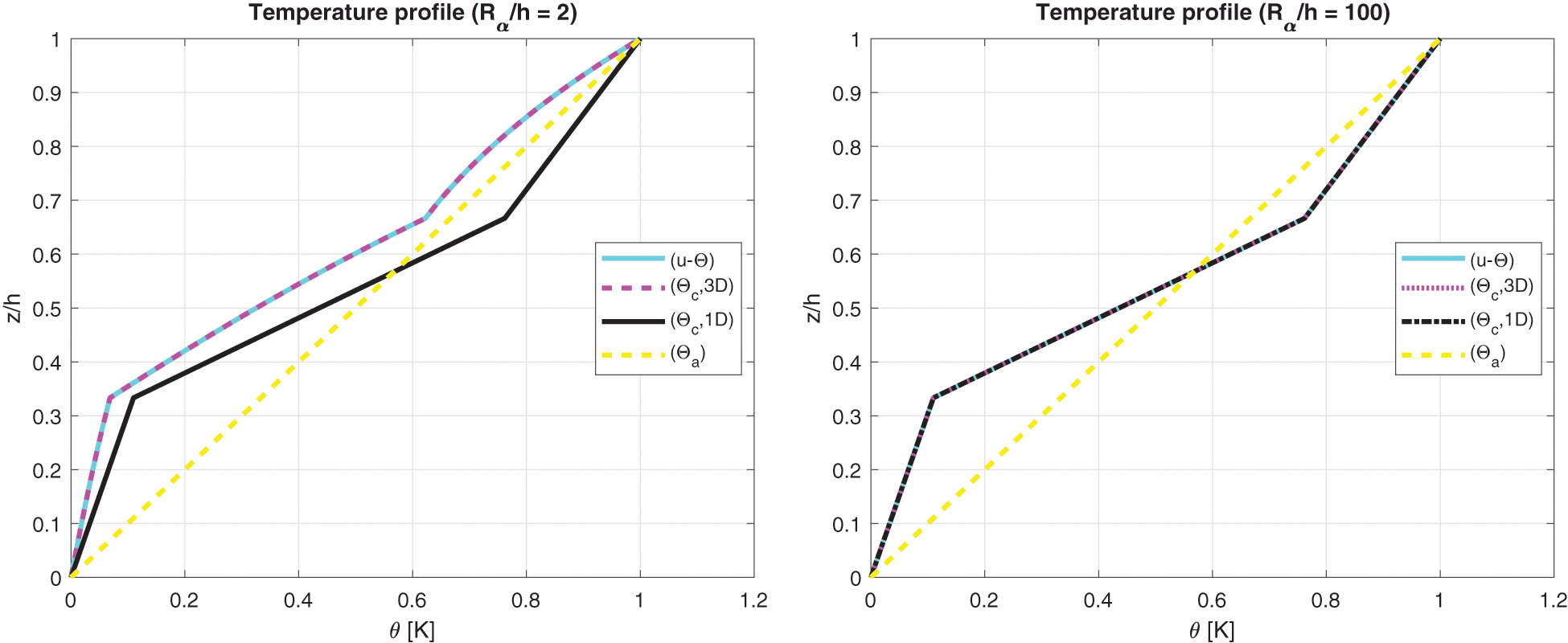
Figure 16: Benchmark eight, temperature profiles for two different
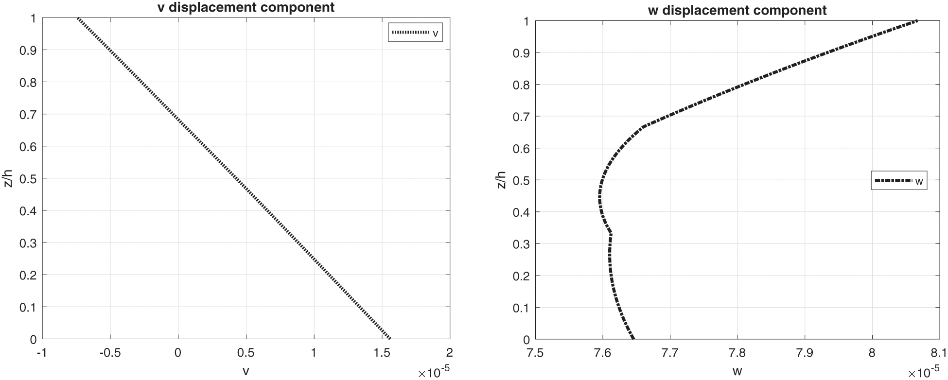
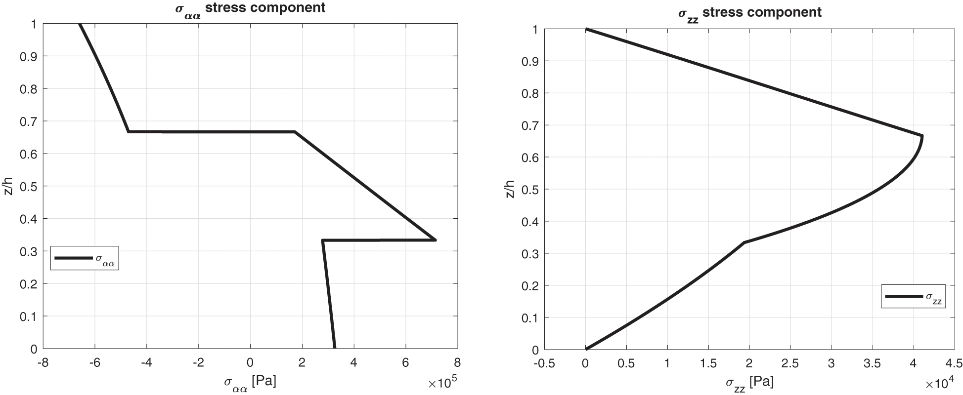
Figure 17: Benchmark eight, displacement components and stress components for a moderately thick spherical shell embedding three isotropic layers (Al2024/Ti22/Steel) (
An overall full coupled thermo-elastic 3D shell model in closed-form solution for the thermal stress investigation of single-and multi-layered isotropic, sandwich and composite plate and shell geometries has been discussed. The sovra-temperature maximum values have been directly applied at the highest and lowest point of outer faces in static conditions. The temperature profile is then evaluated through the thickness direction. The temperature profile is a primary variable as the displacements thanks to the coupling between the 3D Fourier heat conduction equation and the 3D equilibrium equations for shells. This sovra-temperature profile considers both the effects connected with the thickness layer and the embedded material for each possible case, without the necessity to separately solve the 3D or 1D form of the Fourier heat conduction equation. The global coupled system given by the three-dimensional equilibrium equations for shells and the three-dimensional Fourier heat conduction relation for shells is exactly solved via the exponential matrix methodology. Different results, given as displacement components, in-plane and out-of-plane stress components and sovra-temperature evaluations have been discussed for several thickness ratio values, geometrical properties, lamination sequences, temperature impositions and materials. These analyses showed a complete match between the 3D uncoupled model that uses the 3D Fourier heat conduction relation and the 3D full coupled one. This last new method has the advantage that takes into account both the thickness and the material layer effects using a mathematical formulation that is simpler and more elegant because the three-dimensional Fourier heat conduction relation is not separately solved. Moreover, a reduced number of artificial layers M is requested in comparison with the uncoupled 3D model.
Funding Statement: The authors received no specific funding for this study.
Conflict of Interest: The authors declare that they have no conflicts of interest to report regarding the present study.
References
1. Librescu, L., Marzocca, P. (2003). Thermal stresses ’03, vol. 1. Blacksburg, VA, USA: Virginia Polytechnic Institute and State University. [Google Scholar]
2. Librescu, L., Marzocca, P. (2003). Thermal stresses ’03, vol. 2. Blacksburg, VA, USA: Virginia Polytechnic Institute and State University. [Google Scholar]
3. Noor, A. K., Burton, W. S. (1992). Computational models for high-temperature multilayered composite plates and shells. Applied Mechanics Reviews, 45, 419–446. https://doi.org/10.1115/1.3119742 [Google Scholar] [CrossRef]
4. Nowinski, J. L. (1978). Theory of thermoelasticity with applications, vol. 3. The Netherlands: Sijthoff & Noordhoff. [Google Scholar]
5. Altay, G. A., Dökmeci, M. C. (1996). Fundamental variational equations of discontinuous thermopiezoelectric fields. International Journal of Engineering Science, 34(7), 769–782. https://doi.org/10.1016/0020-7225(95)00133-6 [Google Scholar] [CrossRef]
6. Altay, G. A., Dökmeci, M. C. (1996). Some variational principles for linear coupled thermoelasticity. International Journal of Solids and Structures, 33(26), 3937–3948. https://doi.org/10.1016/0020-7683(95)00215-4 [Google Scholar] [CrossRef]
7. Altay, G. A., Dökmeci, M. C. (2001). Coupled thermoelastic shell equations with second sound for high-frequency vibrations of temperature-dependent materials. International Journal of Solids and Structures, 38(16), 2737–2768. https://doi.org/10.1016/S0020-7683(00)00179-7 [Google Scholar] [CrossRef]
8. Cannarozzi, A. A., Ubertini, F. (2001). A mixed variational method for linear coupled thermoelastic analysis. International Journal of Solids and Structures, 38(4), 717–739. https://doi.org/10.1016/S0020-7683(00)00061-5 [Google Scholar] [CrossRef]
9. Das, N. C., Das, S. N., Das, B. (1983). Eigenvalue approach to thermoelasticity. Journal of Thermal Stresses, 6(1), 35–43. https://doi.org/10.1080/01495738308942164 [Google Scholar] [CrossRef]
10. Kosínski, W., Frischmuth, K. (2001). Thermomechanical coupled waves in a nonlinear medium. Wave Motion, 34(1), 131–141. https://doi.org/10.1016/S0165-2125(01)00064-6 [Google Scholar] [CrossRef]
11. Wauer, J. (1996). Free and forced magneto-thermo-elastic vibrations in a conducting plate layer. Journal of Thermal Stresses, 19(7), 671–691. https://doi.org/10.1080/01495739608946201 [Google Scholar] [CrossRef]
12. Bhaskar, K., Varadan, T. K., Ali, J. S. M. (1996). Thermoelastic solution for orthotropic and anisotropic composite laminates. Composites. Part B: Engineering, 27(5), 415–420. https://doi.org/10.1016/1359-8368(96)00005-4 [Google Scholar] [CrossRef]
13. Pagano, N. J. (1969). Exact solutions for composite laminates in cylindrical bending. Journal of Composite Materials, 3(3), 398–411. https://doi.org/10.1177/002199836900300304 [Google Scholar] [CrossRef]
14. Pagano, N. J. (1970). Exact solutions for rectangular bidirectional composites and sandwich plates. Journal of Composite Materials, 4(1), 20–34. https://doi.org/10.1177/002199837000400102 [Google Scholar] [CrossRef]
15. Pagano, N. J., Wang, A. S. D. (1971). Further study of composite laminates under cylindrical bending. Journal of Composite Materials, 5(4), 521–528. https://doi.org/10.1177/002199837100500410 [Google Scholar] [CrossRef]
16. Kulikov, G. M., Plotnikova, S. V. (2015). A sampling surfaces method and its implementation for 3D thermal stress analysis of functionally graded plates. Composite Structures, 120, 315–325. https://doi.org/10.1016/j.compstruct.2014.10.012 [Google Scholar] [CrossRef]
17. Kulikov, G. M., Plotnikova, S. V. (2015). Three-dimensional thermal stress analysis of laminated composite plates with general layups by a sampling surfaces method. European Journal of Mechanics A/Solids, 49, 214–226. https://doi.org/10.1016/j.euromechsol.2014.07.011 [Google Scholar] [CrossRef]
18. Kulikov, G. M., Plotnikova, S. V. (2014). 3D exact thermoelastic analysis of laminated composite shells via sampling surfaces method. Composite Structures, 115, 120–130. https://doi.org/10.1016/j.compstruct.2014.04.019 [Google Scholar] [CrossRef]
19. Savoia, M., Reddy, J. N. (1995). Three-dimensional thermal analysis of laminated composite plates. International Journal of Solids and Structures, 32(5), 593–608. https://doi.org/10.1016/0020-7683(94)00146-N [Google Scholar] [CrossRef]
20. Tungikar, V. B., Rao, K. M. (1995). Three dimensional exact solution of thermal stresses in rectangular composite laminate. Composite Structures, 27(4), 419–430. https://doi.org/10.1016/0263-8223(94)90268-2 [Google Scholar] [CrossRef]
21. Brischetto, S., Torre, R. (2018). Thermo-elastic analysis of multilayered plates and shells based on 1D and 3D heat conduction problems. Composite Structures, 206, 326–353. https://doi.org/10.1016/j.compstruct.2018.08.042 [Google Scholar] [CrossRef]
22. Brischetto, S., Torre, R. (2019). 3D shell model for the thermo-mechanical analysis of FGM structures via imposed and calculated temperature profiles. Aerospace Science and Technology, 85, 125–149. https://doi.org/10.1016/j.ast.2018.12.011 [Google Scholar] [CrossRef]
23. Monge, J. C., Mantari, J. L. (2020). Exact solution of thermo-mechanical analysis of laminated composite and sandwich doubly-curved shell. Composite Structures, 245, 1–14. https://doi.org/10.1016/j.compstruct.2020.112323 [Google Scholar] [CrossRef]
24. Tornabene, F., Brischetto, S. (2018). 3D capability of refined GDQ models for the bending analysis of composite and sandwich plates, spherical and doubly-curved shells. Thin-Walled Structures, 129, 94–124. https://doi.org/10.1016/j.tws.2018.03.021 [Google Scholar] [CrossRef]
25. Brischetto, S., Tornabene, F. (2018). Advanced GDQ models and 3D stress recovery in multilayered plates, spherical and double-curved panels subjected to transverse shear loads. Composites Part B: Engineering, 146, 244–269. https://doi.org/10.1016/j.compositesb.2018.04.019 [Google Scholar] [CrossRef]
26. Alibeigloo, A., Liew, K. M. (2013). Thermoelastic analysis of functionally graded carbon nanotube-reinforced composite plate using theory of elasticity. Composite Structures, 106, 873–881. https://doi.org/10.1016/j.compstruct.2013.07.002 [Google Scholar] [CrossRef]
27. Moleiro, F., Correia, V. M. F., Ferreira, A. J. M., Reddy, J. N. (2019). Fully coupled thermo-mechanical analysis of multilayered plates with embedded FGM skins or core layers using a layerwise mixed model. Composite Structures, 210, 971–996. https://doi.org/10.1016/j.compstruct.2018.11.073 [Google Scholar] [CrossRef]
28. Adineh, M., Kadkhodayan, M. (2017). Three-dimensional thermo-elastic analysis and dynamic response of a multi-directional functionally graded skew plate on elastic foundation. Composites Part B: Engineering, 125, 227–240. https://doi.org/10.1016/j.compositesb.2017.05.070 [Google Scholar] [CrossRef]
29. Rolfes, R., Noack, J., Taeschner, M. (1999). High performance 3D-analysis of thermo-mechanically loaded composite structures. Composite Structures, 46(4), 367–379. https://doi.org/10.1016/S0263-8223(99)00101-4 [Google Scholar] [CrossRef]
30. Thangaratnam, R. K., Palaninathan, R., Ramachandran, J. (1988). Thermal stress analysis of laminated composite plates and shells. Computers & Structures, 30(6), 1403–1411. https://doi.org/10.1016/0045-7949(88)90204-0 [Google Scholar] [CrossRef]
31. Dehghan, M., Nejad, M. Z., Moosaie, A. (2016). Thermo-electro-elastic analysis of functionally graded piezoelectric shells of revolution: Governing equations and solutions for some simple cases. International Journal of Engineering Science, 104, 34–61. [Google Scholar]
32. Padovan, J. (1976). Thermoelasticity of cylindrically anisotropic generally laminated cylinders. Journal of Applied Mechanics, 43, 124–130. [Google Scholar]
33. Trajkovski, D., Cukic, R. (1999). A coupled problem of thermoelastic vibrations of a circular plate with exact boundary conditions. Mechanics Research Communications, 26(2), 217–224. [Google Scholar]
34. Yeh, Y. L. (2005). The effect of thermo-mechanical coupling for a simply supported orthotropic rectangular plate on non-linear dynamics. Thin-Walled Structures, 43(8), 1277–1295. [Google Scholar]
35. Vinyas, M., Kattimani, S. C. (2017). Hygrothermal analysis of magneto-electro-elastic plate using 3D finite element analysis. Composite Structures, 180, 617–637. [Google Scholar]
36. Pantano, A., Averill, R. C. (2000). A 3D zig-zag sublaminate model for analysis of thermal stresses in laminated composite and sandwich plates. Journal of Sandwich Structures & Materials, 2(3), 288–312. [Google Scholar]
37. Khare, R. K., Kant, T., Garg, A. K. (2003). Closed-form thermo-mechanical solutions of higher-order theories of cross-ply laminated shallow shells. Composite Structures, 59(3), 313–340. [Google Scholar]
38. Khdeir, A. A., Reddy, J. N. (1991). Thermal stresses and deflections of cross-ply laminated plates using refined plate theories. Journal of Thermal Stresses, 14(4), 419–438. [Google Scholar]
39. Khdeir, A. A., Reddy, J. N. (1991). Thermal effects on the response of cross-ply laminated shallow shells. International Journal of Solids and Structures, 29(5), 653–667. [Google Scholar]
40. Kalam, M. A., Tauchert, T. R. (1978). Stresses in an orthotropic elastic cylinder due to a plane temperature distribution T(r,
41. He, J. F. (1995). Thermoelastic analysis of laminated plates including transverse shear deformation effects. Composite Structures, 30(1), 51–59. https://doi.org/10.1016/0263-8223(94)00026-3 [Google Scholar] [CrossRef]
42. Ali, J. S. M., Bhaskar, K., Varadan, T. K. (1999). A new theory for accurate thermal/mechanical flexural analysis of symmetric laminated plates. Composite Structures, 45(3), 227–232. https://doi.org/10.1016/S0263-8223(99)00028-8 [Google Scholar] [CrossRef]
43. Brischetto, S. (2009). Effect of the through-the-thickness temperature distribution on the response of layered and composite shells. International Journal of Applied Mechanics, 1(4), 581–605. https://doi.org/10.1142/S1758825109000393 [Google Scholar] [CrossRef]
44. Brischetto, S., Carrera, E. (2010). Coupled thermo-mechanical analysis of one-layered and multilayered isotropic and composite shells. Computer Modeling in Engineering & Sciences, 56(3), 249–302. https://doi.org/10.3970/cmes.2010.056.249 [Google Scholar] [CrossRef]
45. Brischetto, S., Carrera, E. (2010). Coupled thermo-mechanical analysis of one-layered and multilayered plates. Composite Structures, 92(8), 1793–1812. https://doi.org/10.1016/j.compstruct.2010.01.020 [Google Scholar] [CrossRef]
46. Miller, C. J., Millavec, W. A., Kicher, T. P. (1981). Thermal stress analysis of layered cylindrical shells. AIAA Journal, 19(4), 523–530. https://doi.org/10.2514/3.7790 [Google Scholar] [CrossRef]
47. Cheng, Z. Q., Batra, R. C. (2001). Thermal effects on laminated composite shells containing interfacial imperfections. Composite Structures, 52(1), 3–11. https://doi.org/10.1016/S0263-8223(00)00197-5 [Google Scholar] [CrossRef]
48. Barut, A., Madenci, E., Tessler, A. (2000). Nonlinear thermoelastic analysis of composite panels under non-uniform temperature distribution. International Journal of Solids and Structures, 37(27), 3681–3713. https://doi.org/10.1016/S0020-7683(99)00119-5 [Google Scholar] [CrossRef]
49. Huang, N. N., Tauchert, T. R. (1991). Large deflections of laminated cylindrical and doubly-curved panels under thermal loading. Computers & Structures, 41(2), 303–312. https://doi.org/10.1016/0045-7949(91)90433-M [Google Scholar] [CrossRef]
50. Noor, A. K., Peters, J. M. (1999). Analysis of curved sandwich panels with cutouts subjected to combined temperature gradient and mechanical loads. Journal of Sandwich Structures and Materials, 1(1), 42–59. https://doi.org/10.1177/109963629900100103 [Google Scholar] [CrossRef]
51. Raju, K. K., Rao, G. V. (1984). Finite element analysis of thermal postbuckling of tapered columns. Computer & Structures, 19(4), 617–620. https://doi.org/10.1016/0045-7949(84)90108-1 [Google Scholar] [CrossRef]
52. Daneshjoo, K., Ramezani, M. (2002). Coupled thermoelasticity in laminated composite plates based on green-lindsay model. Composite Structures, 55(4), 387–392. https://doi.org/10.1016/S0263-8223(01)00164-7 [Google Scholar] [CrossRef]
53. Daneshjoo, K., Ramezani, M. (2004). Classical coupled thermoelasticity in laminated composite plates based on third-order shear deformation theory. Composite Structures, 64(3–4), 369–375. https://doi.org/10.1016/j.compstruct.2003.09.039 [Google Scholar] [CrossRef]
54. Ibrahimbegovic, A., Colliat, J. B., Davenne, L. (2005). Thermomechanical coupling in folded plates and non-smooth shells. Computer Methods in Applied Mechanics Engineering, 194(21–24), 2686–2707. https://doi.org/10.1016/j.cma.2004.07.052 [Google Scholar] [CrossRef]
55. Lee, Z. Y. (2006). Generalized coupled transient thermoelastic problem of multilayered hollow cylinder with hybrid boundary conditions. International Communications in Heat and Mass Transfer, 33(4), 518–528. https://doi.org/10.1016/j.icheatmasstransfer.2006.01.001 [Google Scholar] [CrossRef]
56. Oh, J., Cho, M. (2004). A finite element based on cubic zig-zag plate theory for the prediction of thermo-electric-mechanical behaviors. International Journal of Solids and Structures, 41(5–6), 1357–1375. https://doi.org/10.1016/j.ijsolstr.2003.10.019 [Google Scholar] [CrossRef]
57. Brischetto, S. (2014). An exact 3D solution for free vibrations of multilayered cross-ply composite and sandwich plates and shells. International Journal of Applied Mechanics, 6(6), 1–42. https://doi.org/10.1142/S1758825114500768 [Google Scholar] [CrossRef]
58. Brischetto, S. (2017). Exact three-dimensional static analysis of single-and multi-layered plates and shells. Composites Part B: Engineering, 119, 230–252. https://doi.org/10.1016/j.compositesb.2017.03.010 [Google Scholar] [CrossRef]
59. Brischetto, S. (2017). A closed-form 3D shell solution for multilayered structures subjected to different load combinations. Aerospace Science and Technology, 70, 29–46. https://doi.org/10.1016/j.ast.2017.07.040 [Google Scholar] [CrossRef]
60. Özişik, M. N. (1993). Heat conduction. New York: John Wiley & Sons, Inc. [Google Scholar]
61. Povstenko, Y. (2015). Fractional thermoelasticity. Switzerland: Springer International Publishing. [Google Scholar]
62. Moon, P., Spencer, D. E. (1988). Field theory handbook: Including coordinate systems, differential equations and their solutions. Berlin: Springer-Verlag. [Google Scholar]
63. Mikhailov, M. D., Özişik, M. N. (1984). Unified analysis and solutions of heat and mass diffusion. New York: Dover Publications Inc. [Google Scholar]
64. Arfken, G. B., Weber, H. J. (2005). Mathematical methods for physicists, Sixth edition. San Diego, USA: Elsevier Academic Press. [Google Scholar]
65. Morse, P. M., Feshbach, H. (1953). Methods of theoretical physics. USA: McGraw-Hill. [Google Scholar]
66. Boyce, W. E., Prima, R. C. D. (2001). Elementary differential equations and boundary value problems. New York: John Wiley & Sons, Ltd. [Google Scholar]
67. Systems of differential equations (2013). http://www.math.utah.edu/gustafso/ [Google Scholar]
Cite This Article
 Copyright © 2023 The Author(s). Published by Tech Science Press.
This work is licensed under a Creative Commons Attribution 4.0 International License , which permits unrestricted use, distribution, and reproduction in any medium, provided the original work is properly cited.
 Downloads
 Citation Tools