Super-Resolution Based on Curvelet Transform and Sparse Representation

1  Introduction

With the existence of high-definition displays (e.g., 1920*1080 for High-definition television and the smart mobile devices 2048*1536), we cannot disregard the necessity of preprocessing techniques like resolution improvement for many applications for robust performance. It is still necessary, especially in remote sensing imaging applications, such as geospatial information systems (G.I.S.), astronomy, geology, ecology studies, etc. High-resolution images (H.R.) are highly demanded analysis for remote sensing images. However, it is consistently distorted due to the sensor’s device limitations or because of imaging environments and capturing circumstances. These circumstances are like atmospheric disturbance, the din of an imaging system, and an optical system aberration. That leads to difficulty obtaining an image with desired resolution appearance due to the expensive production cost for replacing the current hardware devices in the imaging systems and the existence of a massive number of low-resolution (L.R.) images. A preprocessing enhancement technique for image resolution should take place.

Recently, Super-Resolution (S.R.) awarded a lot of awareness. The super-resolution technology’s main objective is to acquire and reconstruct an image with higher resolution from one single L.R. image [1–4] or a series of L.R. images [5–8]. The idea is to increase the quality of the images and improve it before any visual assessment. S.R. technology firstly was proposed in the 1960s by Harris [9] and Goodman [10]. Their work aimed to utilize one L.R. image and its components to reconstruct an image with more information (H.R. image). The reconstruction from a series of L.R. images was introduced in 1984 by Tsai [11]. It’s a cost-effective decision that is important in processing remote sensing or airborne images acquired by radar or optical sensors. Super-resolution techniques can be categorized into the interpolation-based S.R., the reconstructed (multi images) based S.R., and the learning-based S.R. that uses dictionary learning or the new research using deep learning [12,13]. Super-resolution interpolation methods can be parametric or non-parametric methods that estimate the unbeknown pixel’s value from the known ones. They perform well in the low-frequency components but are dis-satisfactory in high-frequency components, which leads to a loss in those high-frequency components (edges). It caused a smoothness in the resulted interpolated image. Therefore, various super-resolution techniques developed based on interpolation in the wavelet domain were used broadly to improve the resolution and make the pixels increase in digital images, leading to an increase in the image resolution (resampling to a more significant number of pixels).

In [14], Anbarjafari et al. applied dual-tree complex wavelet transform (DT-CWT). Their algorithm’s results proved better than applying the bi-cubic interpolation or applying the wavelet zero-padding (W.Z.P.). In [15], Anbarjafari et al. used discrete wavelet transform (DWT) that enhanced edges by adding an intermediary stage using stationary wavelet transform (S.W.T.). Their result was better than using the wavelet zero padding (W.Z.P.) and complex wavelet transform (CWT).

In [16], Anbarjafari et al. used discrete wavelet transform (DWT) and subtracted the original L.R. image from the interpolated low-low (approximation) sub-band to get the difference between them instead of using the L.R. image directly. The results were sharper than wavelet zero padding (W.Z.P.), bi-cubic interpolation, and W.Z.P. using cycle spinning (C.S.).

In [17], Chavez-Roman et al. used a Nonlocal mean (NLM) filter to preprocess. They applied discrete wavelet transform (DWT) and took the differences between the interpolated low-low (approximation) sub-band and the original image. In addition, they used the edge extraction stage. Their results outperform many algorithms such as discrete wavelet transform (DWT), dual-tree complex wavelet transform (DT-CWT), and DWT with the S.W.T. algorithm.

In [18], Ghafoor et al. used DT-CWT with the NLM filter and Lanczos interpolating. Results show outstanding performance over the conventional techniques.

In [19] Zhou et al. used a two-dimensional discrete wavelet transform (2D-DWT). For high-frequency sub-bands, they applied resampling with zero paddings by Fourier transform instead of applying bi-cubic interpolation. The results have the same luminosity as the original image, and high-frequency components are clearer.

In [20] Selen et al. preserved the high-frequency details of the image using discrete wavelet transform (DWT) and sparse representation to reconstruct H.R. image by K- Singular Value Decomposition (K-SVD) dictionaries. They used the approximation sub-band to estimate a more detailed resolved image as an additional intermediate process.

The curvelet transform performs a considerable role in many image processing applications, which is considered a generalization of the wavelet transform with multi-dimensional, that is formulated to plot images at various scales and angles with a few numbers of coefficients.

In [21], Haddad et al. applied the curvelet transform on the low-resolution image. They applied a nonlinear function to enhance the content of all the sub-bands produced by the curvelet transformation. In addition, the interpolated input image and the estimated enhanced image that resulted from using inverse curvelet transform are combined using image fusion. The authors mentioned that using the step of image fusion could increase the enhancement of the resulted image. They reported that their results were better than using the combination of DWT and S.W.T.

In [22], Patil et al. used a curvelet-based interpolation scheme on the rotated grid of two adjacent low-resolution frames (multi L.R. image). Those adjacent frames were obtained by using half-pixel shift image registration to create the high-resolution one.

Super-Resolution methods that utilize sparse representation achieve remarkable success in processing remote sensing images. That is because it makes use of the learned dictionaries that are trained over many tested patches examples. To regularize a super-resolution problem, sparse representation is used. In [23], Liu et al. proposed a super-resolution framework for remote sensing images via sparse representation by building dictionaries that used different types of features. They have extracted three different types of features instead of extracting only one feature.

The preponderant challenge here is to develop an algorithm similar to those algorithms, with significant results. Therefore, in this paper, A modified S.R. algorithm is proposed. It generates a high-resolution image from a single L.R. one. The proposed S.R. algorithm combines the interpolation-based method with the example-based method to produce better results with a sharper view. The performance of the proposed S.R. algorithm was tested and evaluated using numerous L.R. images in [24,25] databases.

The rest of the paper is organized as follows. Section 2 introduces the curvelet image super-resolution methodology. Section 3 is dedicated to the proposed S.R. algorithm. The experimental results are discussed in Section 4. Finally, the work has been concluded in Section 5.

2  Curvelet Super Resolution Methodology

2.1 Pre-processing by NLM Filtering

Buades et al. [26] introduced a filter for denoising natural images that are corrupted by additive Gaussian noise. The Nonlocal mean (NLM) filter is a simple and efficient method for image denoising. It has been used as a prior to reducing annoying artifacts. It has the ability to increase the signal-to-noise ratio (SNR). It is generally assumed that the pixels tend to duplicate themselves with some similar neighbors. Therefore, similar patches in different positions are perceived as multi observations of the desired patch that is used to regularize the image’s restoration issue. It calculates the desired pixel by proceeding weighted average for the whole pixels of the image. This process reduced losing details of an image. It is interested in the gray level (radiometric) and the geometrical configuration of every single point in an entire neighborhood. This permits a great comparison over other neighborhood filters. Non-local mean filter computes a denoised image NL[v](i) of a noisy image v = v(i)|i ∈ I as.

NL[v](i)=∑j∈I⁡w(i,j)v(i) (1)

where the weights w(i,j) can be computed as:

w(i,j)=1z(i)e−Di,jh2 (2)

z(i)=∑j⁡e−∥v(Ni)−v(Nj)∥2,a2h2 (3)

Di,j=∥v(Ni)−v(Nj)∥2,a2 (4)

Weights w(i, j) stands on the similarity between the pixels i and j, w(i, j) should meet the conditions 0≤w(i,j)≤1 and ∑w(i,j)=1. This similarity is based on the radiometric and geometric similarity of the pixels. Pixels with similarly grey levels have larger weights in the average.

Z(i) is a normalizing constant. Di,j is the weighted Euclidean distance that is computed as the distance between two intensity gray level vectors (v( Ni ) and v( Nj ) for the pixel i and j respectively) in high dimensional space, with a Gaussian kernel (a > 0) which is the standard deviation of the Gaussian kernel, h is the filtering degree that monitoring the decay of the exponential and also the decay of the weights as a function of Euclidean distances.

2.2 Curvelet Transform

Curvelet transform was proposed in 2006 by Candes et al. [27]. They proposed a curvelet to transform the signal into a multi-scale representation. It represents objects with uniqueness along curves more accurately than other transforms, using the smallest number of coefficients to reconstruct image details (edges). It’s formulated to plot images at various scales and angles. It overcomes the missing directional selectivity of wavelets. By translation and rotation of a mother curvelet θj , at orientation θl , scale 2 − j and position Xk(i,j) = Rθ−1 ( K1 . 2 − j, K2 .2 − j / 2) we obtain:

φi,j,k(X)=φj(Rθl(X−Xkj,l)) (5)

where Rθ is the rotation by θl radians, and θl is the rotation angles θl = 2π. 2 − j / 2 with l = 0; 1; … such that (0 ≤ θl < 2π) and K is the parameters of translation where K = ( K1 , K2 ) ∈ Z2 thus by taking the dot product of f ϵ L2(R2) and a curvelet θj ,l,k, then curvelet coefficient can be given by

c(j,l,k)=∫f(x)φj,l,k(X)dx (6)

Based on [27], two different discrete curvelet transform algorithms were proposed. The Unequally Spaced Fast Fourier Transform (USFFT) depends on sampling Fourier coefficients of the input image to find the curvelet coefficients. Wrapping transform makes the translation to the curvelets at every scale and angle. However, both algorithms have the same results. The wrapping computation time is shorter than the USFFT. The implementation of curvelets via wrapping treated a 2D image as an input with a cartesian form f [n1, n2]. Wrapping starts with applying Fast Fourier Transform (FFT) to obtain Fourier samples of an image. For every scale and angle resample (interpolate) the Fourier samples, then multiply the interpolated function with a window function to wrap over the origin. After that, it uses the inverse 2D Fast Fourier Transform to obtain the discrete coefficients as in Fig. 1. we can calculate the discrete coefficients as follows:

c(j,l,k1,k2)=∑0≤m≤M,0≤n≤N⁡f[m,n]φj,l,k1,k2[m,n] (7)

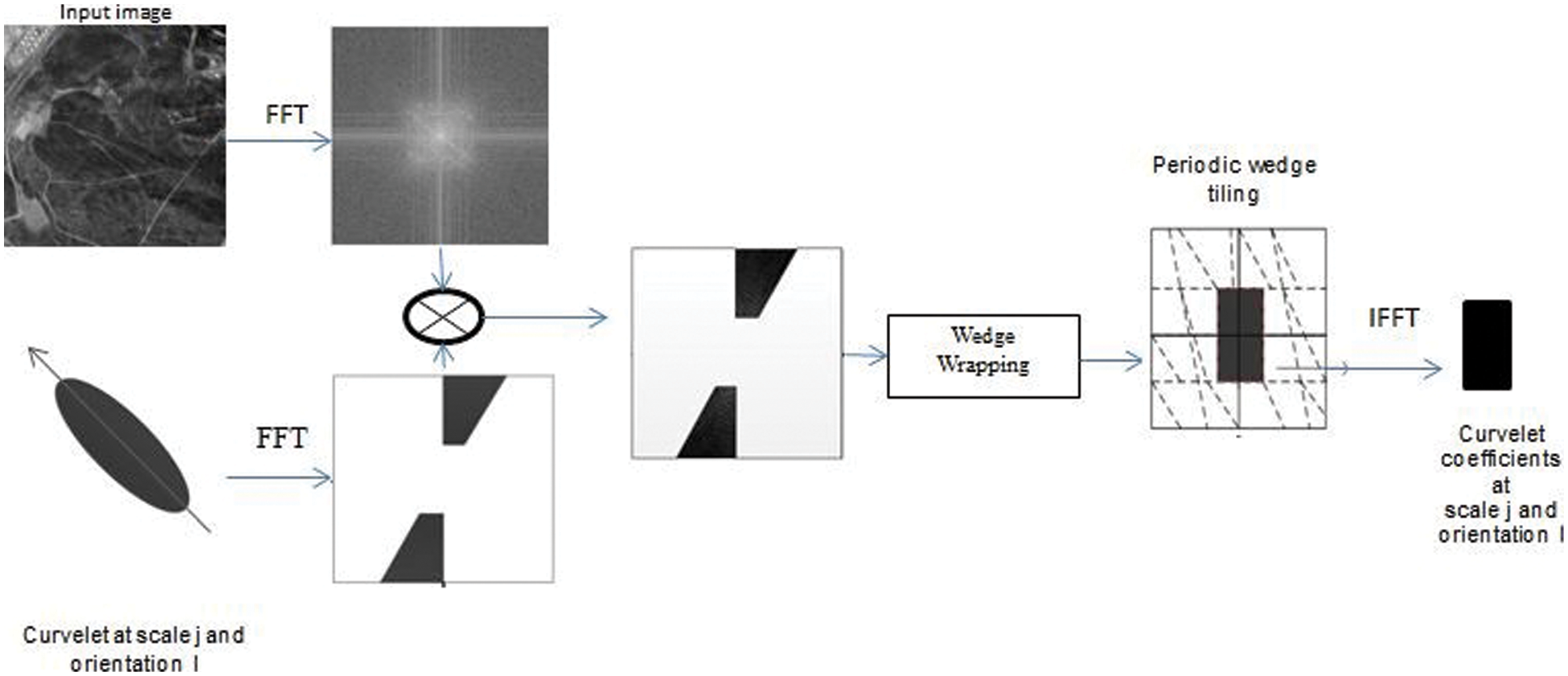
Figure 1: FDCT via wrapping

Eq. (7) calculates c(j, l, K1 , K2 ), which are the discrete curvelet coefficients. Here j, l, K1, and K2 , are the scale, orientation, spatial and location parameters, respectively. ϕ(j, l, K1 , K2 ) is the waveform. It’s noticed that results may be complex. But, we will use their norm.

2.3 Lancozos Interpolation

Lanczos is an interpolation function that performs multi-dimensional interpolation. It has been used broadly in digital signal processing (Lanczos is an alternative to sinc interpolation). It affords great results throughout other interpolations [28]. Lanczos interpolation has the advantage of higher accuracy for sub-pixel better details preservation of small-scale structures. In addition, it better conserves the amplitude (consequently the intensity) and less aliasing artifacts. Lanczos function is given as:

L(X)={1x=0asin(πx)sin(πxa)/asin(πx)sin(πxa)π2X2π2X20otherwise0<|X|<a (8)

where ‘a’ is the order of Lanczos kernel (it can be 2 or 3). This Lanczos kernel gives (2a − 1) lobes. There is an absolute lobe that is placed in the center. In addition, there are (a-1) lobes on each side for negative and positive alternately [29].

Lanczos interpolation depends on the order of its kernel. If the order of the kernel is 2, then 16 neighboring pixels are considered for interpolation, and if the order is 3, then 36 neighboring pixels are utilized [30].

Lanczos keeps most of the contents of the original image. The order of the Lanczos kernel is proportional to the quality of the interpolation. The high order of the kernel yields a high quality of the interpolation.

2.4 Sparse Representation

Recovering a higher resolution image from only one L.R. image is an ill-posed problem. The sparse representation proved an efficacious trend in reconstructing high-resolution images. Solving S.R. problems using sparse representation algorithms [31–36] is effective, especially for a single image. Since the representation is purposed to be sparse, the learned dictionaries are over complete (redundant), making the representation’s quality better. Many algorithms for the sparse representation suppose that the H.R. and L.R. patches share the same set of sparse coefficients. By combining these sparse coefficients for L.R. with the trained H.R. dictionary, we can reconstruct the H.R. image. Firstly, the sparse representation algorithms extract the feature/s in the feature extraction stage. Then the sparse representation stage is responsible for building and learning the dictionaries. Finally, sparse representation produces the H.R. image in the reconstruction stage [31], as clarified in Fig. 2.

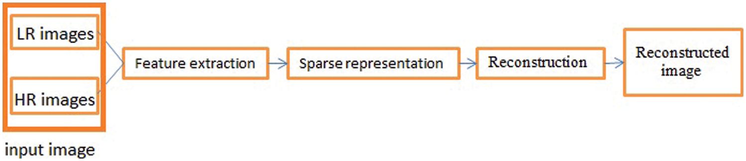
Figure 2: Block diagram of S.R. with sparse representation

To represent an image effectively, we should obtain its essential features using the feature extraction stage, then build the H.R. and L.R. dictionaries by those features. The sparse representation produced the feature patches of the L.R. Finally, it reconstructed the H.R. by integrating the H.R. dictionary with its corresponding L.R. patches’ sparse coefficients. H.R. patches are reassembled to get the H.R. image. Let the L.R. be Y, a blurred form of the H.R. image X.

Y=HBX (9)

where Y and X are the L.R. and H.R. images, respectively, and B is the blur operator. The feature map(s) for the L.R. image that is extracted from Y, can be given by:

Yfeatures=featuresj(Y) (10)

where featuresl (.) is the L.R. feature, extraction operator. The first and second derivatives are usually used as the feature extraction operator [37]. The feature map(s) for the H.R. image that is extracted from X can be given by:

Xfeatures=featuresh(X) (11)

Also, featuresh (.) is the H.R. feature extraction operator, the variation among the L.R. and H.R. image used here as the feature extraction operator. The sparse representation essential units are the patches. Assume that y is the L.R. patch of the feature map, then we get:

Yi=Ri(Yfeature) (12)

Where Ri () extracts the patch from the feature map y feature at position i. Also, the corresponding H.R. patch xi can be given by

Xi=Ri(Xfeature) (13)

The feature patches for L.R. and H.R. ( yi and xi ) are remodeled into feature vectors. Then preparing a training set of { yi , xi }, i = 1, 2, .., M . M is the pairs patches’ number for the L.R. and H.R., then the dictionaries of the L.R. and H.R. are created by using K Singular Value Decomposition (K-SVD) [33]. Dl that refers to the L.R. dictionaries that are computed as:

minDl∑i⁡‖Xi−Dlαli‖22 (14)

where αli is the sparse coefficients for L.R. patch yi , and ||.||1 is the l1 norm. The L.R. and its corresponding H.R. patches are assumed to have symmetric features. So they share the same sparse coefficients that can be expressed as αli=αhi . Thus, H.R. dictionary Dh can be calculated as:

minDh∑i⁡‖Xi−Dlαli‖22 (15)

The main idea of the sparse representation in testing L.R. patch yti in the tested image is depicted by the atom’s linear combination in the L.R. dictionary Dl as yti ≈ Dlαli . Using this assumption, the estimation of the H.R. patch xti of L.R. patch yi with sparse representation by: xti ≈ Dlαli After learning the sparse coefficients αli for every L.R. patch, we use them, and also for the sparse representation to get the corresponding H.R. patch. Whereas all the H.R. patches are gained, averaging all of these patches, the H.R. image is produced.

3  Proposed Super-Resolution Algorithm

Single super-resolution techniques aimed to recover more information (H.R. details) of an image which are unnoticeable in the L.R. image. This paper proposed an algorithm to obtain a super-resolution image from an observed low-resolution one.

Firstly, to reduce the edge artifacts and repress the noise effect on a single L.R. remote sensing image, we have used a Non-local mean filter (NLM) as shown in Step 1, Fig. 3. The NLM depends on the weighted average for the gray values of the whole pixels in an entire image to restore the estimated pixel’s gray value. In this work, we have used the noise level σ = 10, the search window (S.W.) of 17*17 pixels, and the patch window (P.W.) of 9*9 pixels as the optimal results as tested in [38].

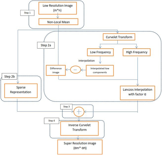
Figure 3: The proposed super-resolution algorithm main steps

Since edges of an image are curved rather than being straight. Therefore, applying curvelet transform is more specific to obtain a typical representation of the smoothed objects (low frequency) and edges (high frequency). Here we have used the digital wrapping curvelet transform as illustrated in Step 2a in Fig. 3, as follows:

1.    Applying 2D Fast Fourier Transform to get Fourier samples as

F[n1,n2],(−n)/2≤n1,n2]≤n/2

2.    For all scales j and orientations l, find the product (interpolation) Uj,l [n1, n2].f^[n1, n2]

3.    Wrapping around the origin f^j,l[n1, n2] = W (Uj,l.f^)[n1, n2]

4.    Apply inverse 2D-FFT to each f^j,l, to get the discrete coefficient.

Lanczos interpolation is applied to all high frequency (H.F.) components to keep the amplitude of sub-pixels. An additional process was applied: the difference between the original image and the interpolated low frequency (L.F.) components. It will be in a high-frequency version. This is an intermediary process to enhance the appreciated high-frequency components.

Super-resolution techniques that are based on sparse representation proved eligibility in recovering H.R. remote sensing images. Here, the input for the sparse representation in step 2b in Fig. 3 is the denoised image resulting from step 1. In Sparse representation, features are extracted. Derivative features [36] are commonly used in super-resolution fields. To represent a remote sensing image here, we used the second derivative. Eqs. (12) and (13) are used to construct the feature patches to build H.R. and L.R. dictionaries.

For each patch, the sparse representation coefficients are calculated in the sparse representation. The H.R. patches are estimated by training H.R. and L.R. dictionaries and sparse coefficients for reconstruction. Then the H.R. dictionary and its corresponding L.R. spares’ coefficients patches are used to reconstruct the H.R. patches, reuniting all the H.R. patches to recover the output image.

The result for the interpolations and the sparse representation image are combined in step 3 in Fig. 3. It is then introduced to the inverse curvelet transform in step 4 in Fig. 3 to get the final reconstructed H.R. image. The obtained results show that the H.R. image is brightened up to clarify the superior of the proposed S.R. algorithm. Fig. 3 displays the main steps of the proposed S.R. algorithm.

To evaluate the proposed S.R. algorithm, experiments are performed on aerial optical and radar images [24,25]. We used 100 down-sampling images of size 128*128 pixels as input images, the training set was 70 images, and 30 were used as a testing set. With dictionary size 1024, for both L.R. and H.R. dictionaries. Patches size was 5*5 pixels for both dictionaries as tested in [31].

4  Experimental Results

The experimental results for the proposed S.R. algorithm have been applied over two different datasets, one for the University of Southern California-Signal and image processing institute (USC-SIPI) and the second Spaceborne Imaging Radar-C/X-Band Synthetic Aperture Radar (SIR-C/X- S.A.R.). The USC-SIPI image database in [24] contains 38 high-altitude aerial images, with dimensions between 512 × 512 and 2250 × 2250 pixels. Radar images of SIR-C/X- S.A.R. are described in [25].

These dataset images have different physical characteristics with different dimensions. To form a low-resolution image, down-sampling (lose much information) was applied over 100 original images from both datasets twice, the first time by a factor of 4 on each axis. The obtained images size is 128*128 pixels. The second time was by factor 2 on each axis. The obtained images size is 256*256 pixels.

The proposed S.R. algorithm applied the NLM filter for the down-sampled L.R. images. The denoised image is the input for the sparse representation. Parallels, the same denoised image has been interpolated with curvelet transform. Then the output of the sparse representation and the interpolated resulted image are combined with the inverse curvelet transform to get the final H.R. image. The evaluation for the proposed S.R. algorithm has been done through two phases. The first phase is used to evaluate the sparse representation step. The sparse representation step used 100 images of size (128*128) pixels as input images. The training set was 70 images, and the testing set (not in the training set) was 30 images. The dictionary size for both L.R. and H.R. dictionaries was 1024 patches. The patches size was (5*5) pixels for both dictionaries. The second phase is used to evaluate the final results of the overall proposed S.R. algorithm. The proposed algorithm has been evaluated through quality measures and visual observation. The quality measure is described as follows.

4.1 Quality Measures

The quality measures that are undertaken via objective metrics Mean Absolute Error (M.A.E.), Peak Signal to Noise Ratio (PSNR), and Structural Similarity Index Measure (SSIM) [39] are defined by the following equations:

MAE=∑i=1n⁡|yi−Xi|/∑i=1n⁡|yi−Xi|nn (16)

PSNR=10logmaxi2/maxi2MSEMSE (17)

SSIM=[ l(x,y)α.c(x,y)β.s(x,y)γ ] (18)

where yi is the resulted image, Xi is the original image, n is the number of pixels, the maxi is the maximum pixels of an image, mean square error ( M .S.E.), the comparison measurements l is luminance, c is contrast and s is structure. Simplifying the equation, assuming that α = β = γ = 1. The evaluation metrics have been recorded for ten images from the above data set twice. When the input image was 128*128 pixels (after down-sampling the original image by factor 4), the resulted image after applying the proposed S.R. algorithm becomes 512*512 pixels. Another time when the input image was 256*256 pixels (after down-sampling the original image by factor 2), the resulted image after applying the proposed S.R. algorithm becomes 512*512 pixels. Tab. 1 presents the evaluation metric of the resulted 512*512 pixels H.R. images after applying the proposed S.R. algorithm by factor 4). Tab. 2 presents the evaluation metric of the resulted 512*512 pixels H.R. images after applying the proposed S.R. algorithm by factor 2). We notice that the calculated M.A.E. value for all tested images is minimal, which means that the average absolute difference between the original image (before down-sampling) and the resulted one is too tiny. This makes the resulted image close to the original one. The PSNR values are between 34 and 28; these values are in an acceptable range. This implies that the quality of the reconstructed image has been improved. In addition, SSIM is closed to 1; this indicates perfect structural similarity between the reconstructed image and the original image (before down-sampling).

In conclusion, the proposed S.R. algorithm carried out a satisfactory result. This indicates that the proposed S.R. algorithm produces a high-resolution image with enhanced edges. We refer to the achieved improvement of the obtained results due to the combination of sparse representation and the curvelet transform.

Besides the quality measures evaluation, the visual observation for the input L.R. images and the reconstructed H.R. image illustrates that the reconstructed image of the proposed S.R. algorithm is obviously better recovered and contains more information than the input L.R. image.

Fig. 4 shows some examples of original images (512*512), LR image 128*128 (down-sampling), and the resulted H.R. (512*512) from the used datasets with respect to PSNR, SSIM, and M.A.E. The proposed S.R. algorithm restores to some degree the geometrical structures and preserved the fine details preferably. The resulted H.R. image has fewer smoothing and ringing artifacts around the edges. It is clearly sharper than the input L.R. image. Fig. 5 shows some examples of the zoomed section of the original images (128*128) and the zoomed selection of the resulted H.R. images (512*512). The resultant image is enhanced, sharper, and enlarged from 128 × 128 to 512 × 512 (by a factor of 4). The results show better performance of the proposed S.R. algorithm. It better preserves the features, preventing blurization, jaggies, and artifacts around edges.

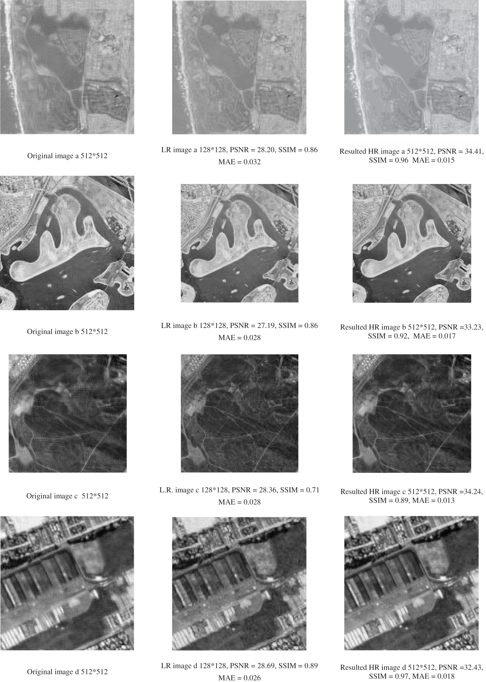
Figure 4: Examples of the S.R. proposed algorithm L.R. image and the resulting H.R. image regarding PSNR, SSIM and M.A.E

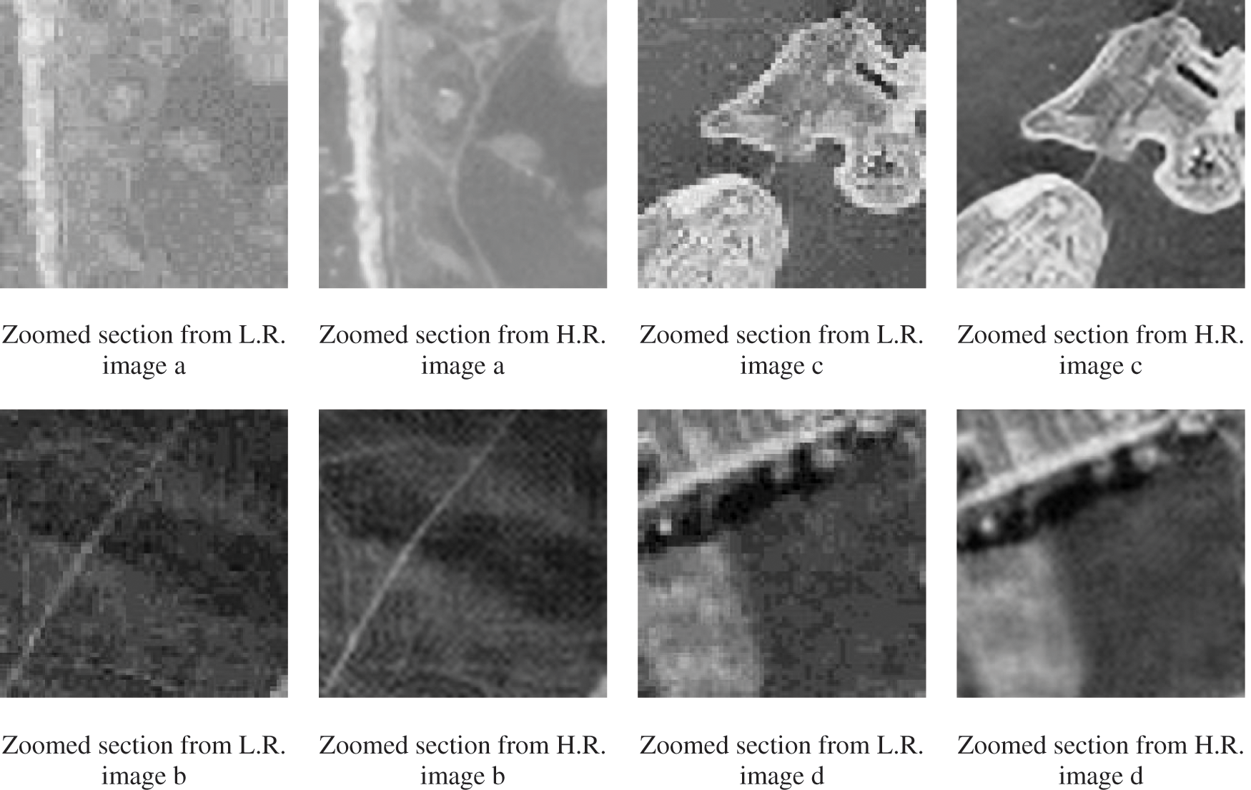
Figure 5: Examples of the S.R. proposed algorithm for original image zoomed section and the resulted zoomed H.R. section

4.2 Comparison with Other Algorithms

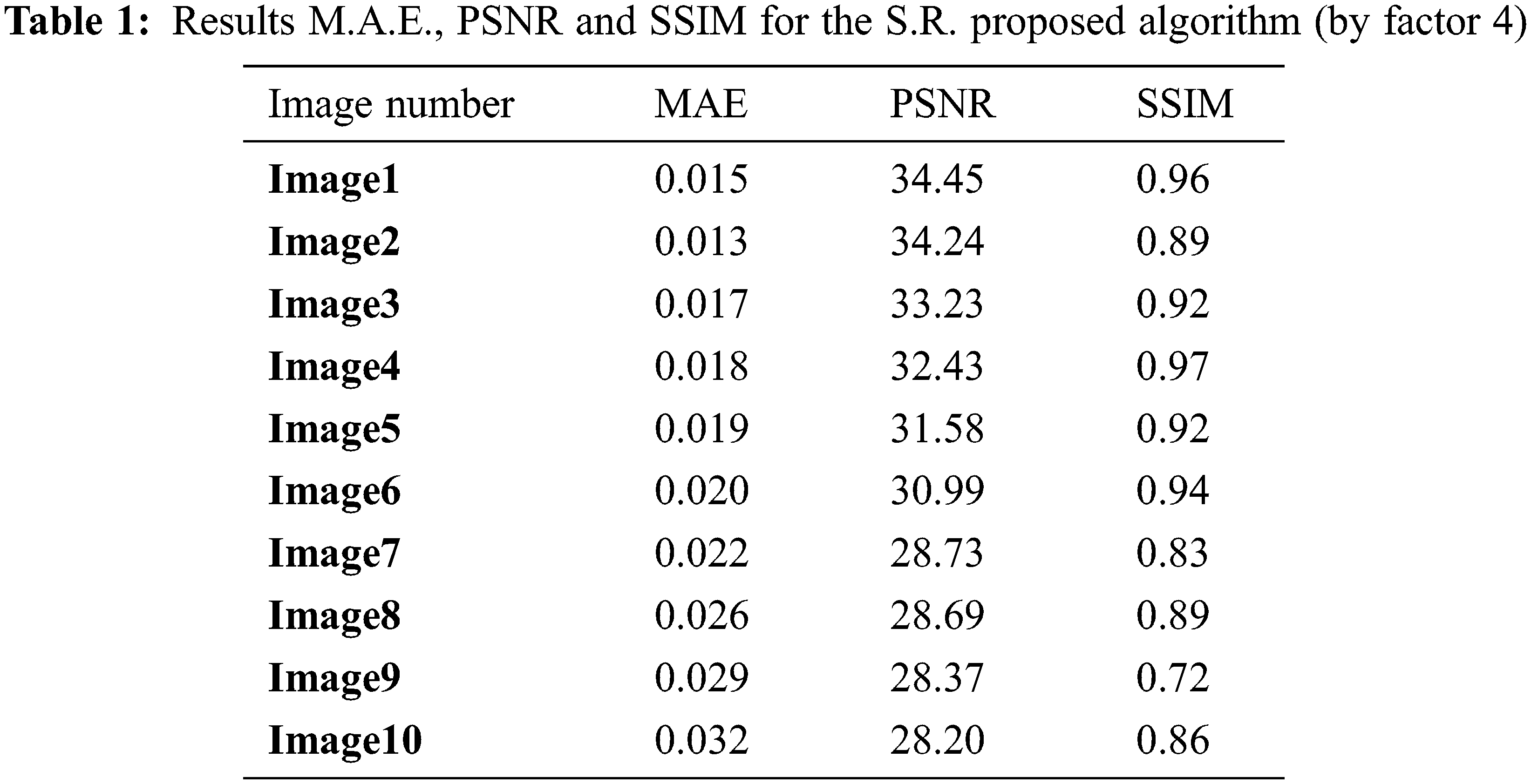
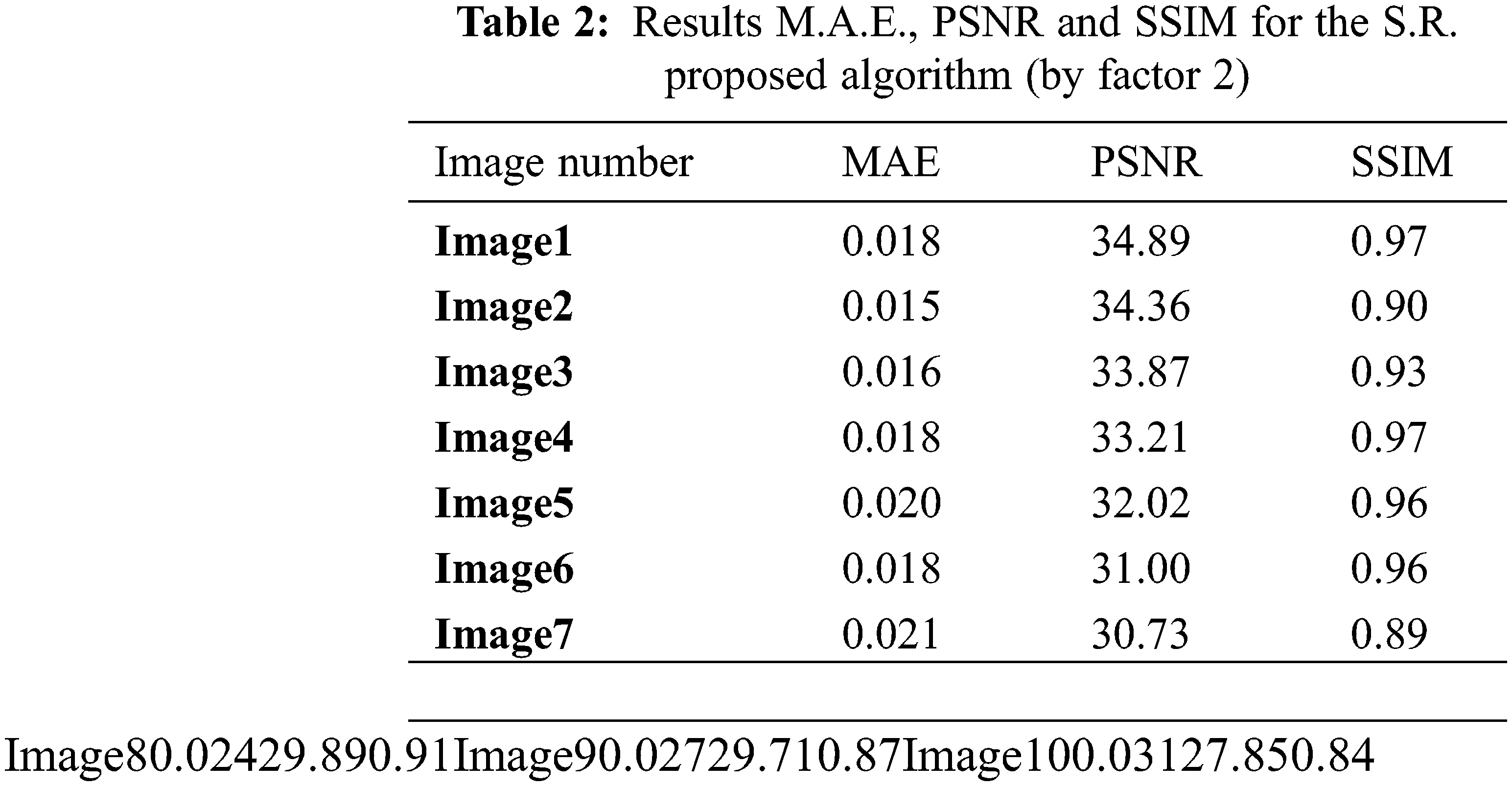
Tab. 3 is a comparison of Demirel et al. 2011 [16], Chavez-Roman et al. 2014 [17], Iqbal et al. 2012 [18], Ayas et al. 2018 [20] and our proposed algorithm with respect to M.A.E., PSNR, and SSIM.

We make the evaluation of average objective criteria values (M.A.E., PSNR, and SSIM) over the images from [24,25]. The resulted HR images have the following: MAE= 0.013, PSNR = 34.45 dB, and SSIM = 0.97. The presented analysis and results show that the proposed S.R. algorithm outperformed other algorithms and achieved a satisfactory improvement. It enlarged the input L.R. images from 128 × 128 to get H.R. images 512 × 512 (by a factor of 4). This indicates that the proposed S.R. algorithm can generate a super-resolution image and furtherly enhance the edges.

5  Conclusion

This paper proposed a super-resolution algorithm based on curvelet transform and sparse representation. It employed the NLM denoising filter as a prior. The recorded results show that using a curvelet with sparse representation achieved superior performance for the proposed S.R. algorithm with respect to M.A.E., PSNR, and SSIM. The comparison study shows that the S.R. algorithm outperforms the conventional algorithms. In addition, the intermediary process of having the difference between the Interpolated low frequency (L.F.) components (that have additional H.F. features) and the original L.R. image produced an appreciably reconstructed S.R. image, which conserves much more high-frequency components.

Acknowledgement: Authors thanks everyone who contributed to the article.

Funding Statement: The authors received no specific funding for this study.

Conflict of Interest: The process of writing and the content of the article does not give grounds for raising the issue of a conflict of interest. The authors have no conflicts of interest to report regarding the present study

Compliance with Ethical Standards: This article is a completely original work of its authors; it has not been published before and will not be sent to other publications until the PRIA editorial board decides not to accept it for publication.

References

 1.  S. Bagon, D. Glasner and M. Irani, “Super-resolution from a single image,” in IEEE 12th Int. Conf. on Computer Vision, Kyoto, pp. 349–356, 2009. [Google Scholar]

 2.  K. I. Kim and Y. Kwon, “Single-image super-resolution using sparse regression and natural image prior,” IEEE Transactions on Pattern Analysis and Machine Intelligence, vol. 32, no. 6, pp. 1127–1133, 2010. [Google Scholar]

 3.  T. S. Huang, Y. Ma, J. Wright and J. Yang, “Image super-resolution via sparse representation,” IEEE Transactions on Image Processing, vol. 19, no. 11, pp. 2861–2873, 2010. [Google Scholar]

 4.  W. T. Freeman, T. R. Jones and E. C. Pasztor, “Example-based super-resolution,” IEEE Computer Graphics and Applications, vol. 22, no. 2, pp. 56–65, 2002. [Google Scholar]

 5.  X. Gao, Y. Hu, X. Li, B. Ning and D. Tao, “A multi-frame image super-resolution method,” Signal Processing, vol. 90, no. 2, pp. 405–414, 2010. [Google Scholar]

 6.  H. Hino, T. Kato and N. Murata, “Multi-frame image super resolution based on sparse coding,” Neural Networks, vol. 66, no. 8, pp. 64–78, 2015. [Google Scholar]

 7.  M. Irani and S. Peleg, “Super resolution from image sequences,” in [1990] Proc. 10th Int. Conf. on Pattern Recognition, IEEE, Atlantic City, NJ, USA, pp. 115–120, 1990. [Google Scholar]

 8.  Q. Liao, W. Yang and F. Zhou, “Interpolation-based image super-resolution using multisurface fitting,” IEEE Transactions on Image Processing, vol. 21, no. 7, pp. 3312–3318, 2012. [Google Scholar]

 9.  L. J. Harris, “Diffraction and resolving power,” Journal of the Optical Society of America, vol. 54, no. 7, pp. 931, 1964. [Google Scholar]

10. J. W. Goodman, Introduction to Fourier optics, 3rd ed., Englewood, Colorado: Roberts & Co. Publishers, 2005. [Google Scholar]

11. R. Tsai, “Multiframe image restoration and registration,” Advance Computer Visual and Image Processing, vol. 1, pp. 317–339, 1984. [Google Scholar]

12. Z. Wang, J. Chen and S. C. H. Hoi, “Deep learning for image super-resolution: A survey,” IEEE Transactions on Pattern Analysis and Machine Intelligence, vol. 43, no. 10, pp. 3365–3387, 2020. [Google Scholar]

13. W. Sun, L. Dai, X. R. Zhang, P. S. Chang and X. Z. He, “RSOD: Real-time small object detection algorithm in UAV-based traffic monitoring,” Applied Intelligence, vol. 92, no. 6, pp. 1–16, 2021. [Google Scholar]

14. G. Anbarjafari and H. Demirel, “Satellite image resolution enhancement using complex wavelet transform,” IEEE Geoscience and Remote Sensing Letters, vol. 7, no. 1, pp. 123–126, 2009. [Google Scholar]

15. G. Anbarjafari and H. Demirel, “Image resolution enhancement by using discrete and stationary wavelet decomposition,” IEEE Transactions on Image Processing, vol. 20, no. 5, pp. 1458– 1460, 2010. [Google Scholar]

16. G. Anbarjafari and H. Demirel, “Discrete wavelet transform-based satellite image resolution enhancement,” IEEE Transactions on Geoscience and Remote Sensing, vol. 49, no. 6, pp. 1997–2004, 2011. [Google Scholar]

17. H. Chavez-Roman and V. Ponomaryov, “Super resolution image generation using wavelet domain interpolation with edge extraction via a sparse representation,” IEEE Geoscience and Remote Sensing Letters, vol. 11, no. 10, pp. 1777–1781, 2014. [Google Scholar]

18. A. Ghafoor, M. Z. Iqbal and A. M. Siddiqui, “Satellite image resolution enhancement using dual-tree complex wavelet transform and nonlocal means,” IEEE Geoscience and Remote Sensing Letters, vol. 10, no. 3, pp. 451–455, 2012. [Google Scholar]

19. C. Zhou and J. Zhou, “Single-frame remote sensing image super-resolution reconstruction algorithm based on two-dimensional wavelet,” in IEEE 3rd Int. Conf. on Image, Vision and Computing (ICIVC), Chongqing, China, pp. 360–363, 2018. [Google Scholar]

20. A. Selen and M. Ekinci, “Single image super resolution based on sparse representation using discrete wavelet transform,” Multimedia Tools and Applications, vol. 77, no. 13, pp. 16685–16698, 2018. [Google Scholar]

21. Z. Haddad, J. L. Krahe and A. C. H. Tong, “Image resolution enhancement based on curvelet transform,” in 12th Int. Conf. on Computer Vision Theory and Applications, Porto, Portugal, pp. 167–173, 2017. [Google Scholar]

22. A. A. Patil, R. Singhai and J. Singhai, “Curvelet transform based super-resolution using sub-pixel image registration,” in 2nd Computer Science and Electronic Engineering Conf. (CEEC), University of Essex, UK, IEEE, pp. 1–6, 2010. [Google Scholar]

23. K. Liu, Y. Liu, W. Wu, X. Yang and B. Yan, “A new framework for remote sensing image super-resolution: sparse representation-based method by processing dictionaries with multi-type features,” Journal of Systems Architecture, vol. 64, pp. 63–75, 2016. [Google Scholar]

24. visited Sep, 2021. [Online]. Available: http://sipi.usc.edu/database/. [Google Scholar]

25. visited Sep, 2021. [Online]. Available: http://www.jpl.nasa.gov/radar/sircxsar/. [Google Scholar]

26. A. Buades, B. Coll and J. M. Morel, “A nonlocal algorithm for image denoising,” in IEEE Computer Society Conference on Computer Vision and Pattern Recognition (CVPR’05), San Diego, California, USA, vol. 2, pp. 60–65, 2005. [Google Scholar]

27. E. Candes, L. Demanet, D. Donoho and L. Ying, “Fast discrete curvelet transforms,” Multiscale Modeling & Simulation, vol. 5, no. 3, pp. 861–899, 2006. [Google Scholar]

28. L. Liang, “Image interpolation by blending kernels,” IEEE Signal Processing Letters, vol. 15, pp. 805–808, 2008. [Google Scholar]

29. A. R. Kumar and S. Safinaz, “VLSI realization of lanczos interpolation for a generic video scaling algorithm,” in Int. Conf. on Recent Advances in Electronics and Communication Technology (ICRAECT), Bangalore, India, pp. 17–23, 2017. [Google Scholar]

30. Lanczos resampling visited Sep, 2021. [Online]. Available: http://en.wikipedia.org/wiki/. [Google Scholar]

31. T. S. Huang, Y. Ma, J. Wright and J. Yang, “Image super-resolution via sparse representation,” IEEE Transactions on Image Processing, vol. 19, no. 11, pp. 2861–2873, 2010. [Google Scholar]

32. X. Li, X. Lu, P. Yan, Y. Yuan and H. Yuan, “Geometry constrained sparse coding for single image super-resolution,” in IEEE Conf. on Computer Vision and Pattern Recognition, Providence, RI, USA, pp. 1648–1655, 2012. [Google Scholar]

33. Y. Liang, Q. Pan, S. Wang and L. Zhang, “Semi-coupled dictionary learning with applications to image super-resolution and photo-sketch synthesis,” in IEEE Conf. on Computer Vision and Pattern Recognition, Providence, RI, USA, pp. 2216–2223, 2012. [Google Scholar]

34. X. Gao, X. Li, D. Tao and K. Zhang, “Multi-scale dictionary for single image super-resolution,” in IEEE Conf. on Computer Vision and Pattern Recognition, Providence, RI, USA, pp. 1114–1121, 2012. [Google Scholar]

35. S. Li and W. Liu, “Multi-morphology image super-resolution via sparse representation,” Neurocomputing, vol. 120, no. 3, pp. 645–654, 2013. [Google Scholar]

36. W. Chen, G. Jeon, W. Wu, B. Yan and X. Yang, “Remote sensing image super-resolution using dual-dictionary pairs based on sparse presentation and multiple features,” in Proc. of Int. Conf. on Internet Multimedia Computing and Service, Xiamen China, pp. 90–94, 2014. [Google Scholar]

37. X. He, Z. Liu and W. Wu, “Learning-based super resolution using kernel partial least squares,” Image and Vision Computing, vol. 29, no. 6, pp. 394–406, 2011. [Google Scholar]

38. F. J. Gallegos-Funes, I. V. Hern'andez-Guti'errez and A. J. Rosales-Silva, “Improved preclassification non local-means (IPNLM) for filtering of grayscale images degraded with additive white Gaussian noise,” EURASIP Journal on Image and Video Processing, vol. 2018, no. 1, pp. 1–14, 2018. [Google Scholar]

39. A. C. Bovik and Z. Wang, “Mean squared error: Love it or leave it? A new look at signal fidelity measures,” IEEE Signal Processing Magazine, vol. 26, no. 1, pp. 98–117, 2009. [Google Scholar]