Selective Harmonics Elimination Technique for Artificial Bee Colony Implementation

1  Introduction

In current decades, self-governing solar-powered VSI have gained a reputation in small and medium-power requirements. Maximum harmonic frequencies in conventional inverters are present because of the power electronic circuit. Harmonics decays the life anticipation of electronic and electrical devices. To decrease harmonic difficulties, multilevel inverters (MLIs) have been created. The MLI lowers the switching pressures and losses in power semiconductor circuits. In the twenty-first century, photovoltaic systems have grown increasingly significant in our life. However, due to temperature and insolation fluctuations, the yield potential in the PV (Photovoltaics) system has high-range ripples and variable output power. The Maximum PowerPoint Tracking (MPPT) algorithm, combined with the appropriate DC to DC converter, overcomes these shortcomings.

Although switching faults and Total Harmonic Distortions are slightly higher in high repetition variation schemes, a sinusoidal switching frequency approach regulates the output voltage of a Multilevel Inverter.These drawbacks are solved by the adaptive Selective Harmonics Elimination (SHE) approach. The following are some examples of previously published works of literature.

Cascaded H-bridge inverters, diode clamped MLI and capacitor clamped MLI are mostly used MLI topologies. As compared to other cascaded MLI give good efficiency due to low volume, low switching misfortunes, solid electromagnetic capacities and brilliant productivity. Symmetric and asymmetric are the two types of cascaded multi-level inverters. Compared with asymmetric, symmetric have more number of switches.

In [1], the researcher introduces symmetrical MLI with a minimum number of switches and obtains high-quality output voltage. To decrease harmonics, the authors in [2,3] employ level-shifted and phase-shifted PWM approaches, although these methods are only suited for low-power applications. MLI [4], a switched capacitor, cuts down on the number of DC (Direct current) voltage sources. The capacitor, on the other hand, poses a voltage stability problem in this scenario. The Selective Harmonics Elimination approach [5] overcomes the problems of high-frequency modulation. However, this inverter isn’t designed for nonlinear loads.

The input voltage from the switched rectifier necessitates a large capacitor bank as well as an EB supply. [6], a PV-based cascaded Sinusoidal pulse width overcomes these drawbacks. However, the level started shifting and the phase moved Duty cycle techniques are used in this paper for control. The recommended inverter’s application areas are reduced using these methods. In [7,8] incorporates boosting gain inverters. However, the number of switches in this configuration is significant, and the control loop is also complicated. A PV-based T-shape inverter was studied in [9]. This inverter is perfect for PV systems that are connected to the power grid. In this project, current source rectifiers-based multilevel inverters with Woman Pulse width modulation are used [10].

A current source rectifier, on the other hand, modifies the nature of the input current while also increasing the power loss. In [11] discusses the many ways of Selective Harmonics Elimination. In the development of future procedures, this methodology will be incredibly useful. To lessen the Harmonics, [12–15] studies the usage of many forms of Selective Harmonics Elimination procedures. Normally Multilevel inverter step angles are frequently determined using optimization techniques [16]. In [17], the author used a Genetic Algorithm (GA) to train the neural network to reduce the harmonics. The switching angles for a five-level inverter were predicted using the Particle Swarm Optimization (PSO) technique in [18,19].

This work look at Selective Harmonics Elimination with a four-quadrant operation. This work uses a four-quadrant procedure to look at Selective Harmonics Elimination to reduce the THD (total harmonic distortion) based on PV-based MLI. The suggested work solves all of the existing issues. In this recommended setup, the solar PV system’s input potential is supplied into a maximum Gain DC-DC SEPIC (Single Ended Primary Inductor Converter) converter. The worldwide optimization procedure based Control signal is used to fine-tune the output voltage. The suggested reduced switch fifteen-level inverter is provided varied output voltages. High-frequency Modulation techniques and Selective Harmonics Elimination methods are used to regulate the inverter. In the result and discussion phase, the Harmonic distortion parameters are seen in the comparison outcome.

2  Proposed System

The proposed PV-powered SPEIC converter with a reduced number of switches in a fifteen-level inverter is shown in Fig. 1.

Figure 1: Proposed system circuit diagram of SEPIC converter

The DC-DC SEPIC Converter receives the PV systems highly changing potential signal, which keeps the source flow constant. For the Multilevel Inverter, the Grey Wolf Optimization approach is employed to generate the required DC yield potential. After comparing the reference and real voltages, the error is delivered to the comparator. The SEPIC Converter’s output is used to determine the actual voltage. The PI controller receives the error. The Control system decreases the error and generates a reference signal that is used to generate PWM. The proportional and integral gains are controlled using the GWO computation. The reference and carrier signals are generated and then compared to create switching frequency pulses.

The Converter Topology receives the PWM (Pulse Width Modulation) signal. Reduced switch Multilevel Inverters receive the SEPIC Converter, which produces three input voltages. A single H-bridge inverter and a voltage amplifier circuit with six semiconductor switches and four DC sources make up the proposed reduced switch multilevel inverter for the fifteen-stage inverter. The multi-carrier modulating technique is used to control MLI. High-frequency modulation is another name for Transpose technology. THD (Total harmonic distortion) and conversion losses are significant in high-frequency modulation techniques. Selective harmonics elimination technique based on particle mass colonies is used to meet these challenges. The level of harmonics is compared to the optimization approach.

2.1 PV Panel Modeling

The PV panel’s signal diode format is shown in Fig. 2.

Figure 2: Single diode format of the PV panel

The photovoltaic panels transform light into electricity. In the “(1),” the solar panel current is

Ipv=Io[e(V+Rs.I)Vk.α−1]V+I.RsRsh (1)

whereas

V & I → Output Voltage and Current.

Io & Ipv → Saturation and Array Current.

Rs → Series Resistance Value.

Vk → Thermal Voltage Range.

Rsh → Shunt Resistance Value.

Three solar panels are connected in the proposed configuration. The SEPIC Converter receives the output from the solar configuration.

2.2 SEPIC Converter

The SEPIC Converter behaves like a chopper because of the step down and up in frequency. This converter can do both voltage buck and boost operations. This conversion also keeps the input current constant, enhancing conversion efficiency. The Converter Topology has a diode that delivers dv/dt protection. Fig. 3 shows the SEPIC Converter’s circuit diagram.

Figure 3: SEPIC converter circuit diagram

The inductor current flow is calculated by using Eq. (2).

ΔIL=Iout.V0.40%Vin (2)

The value of the inductor (L1 and L2 is calculated by using Eq. (3).

L1=L2=Vin.αΔIL×Fsw (3)

The value of DC ripple voltage in the capacitor is calculated using Eq. (4) below.

ΔVcin=IoutCin.FSM(VoutVin+Vout+VD) (4)

The following Eq. (5) is used to calculate the output of the capacitor

Cout=Iout.αΔVCin×0.5×FEW (5)

where

α → SEPIC Converter’s Duty Ratio.

FSW → Carrier signal’s Switching Frequency

The GWO algorithm was created to maintain a steady voltage.

2.3 Grey Wolf Optimization (GWO) Algorithm

The SEPIC Converter’s output voltage VDC is compared to the reference voltage Vreference, and the controller is informed of the mistake (PI). The following formula may be used to calculate the error signal:

ΔVerrror(n)=Vreference(n)+VDe(n) (6)

The output of PI controller is illustrated as,

Ireference=Kp1(ΔVerror(n)−ΔVerror(n−1)+KI1.ΔVerror(n) (7)

The GWO algorithm is used to fine-tune the value of optimized Kp & Ki

The GWO algorithm the work is based on the features of grey wolves in their search for food, as well as the management pyramid and the inhabitant running technique. To replicate the hierarchy, this strategy uses four types of wolves: alpha (α), beta (β), gamma (γ), and omega (ω). The wolf is seen to be the best option, and it is the series’ decision-maker and leader. Because they support the wolf in making decisions, the wolves are the second and third best options, respectively. Finally, the surviving wolves that are pursuing the leaders are referred to as. The algorithm’s aggressive behavior is explained as beneath:

E→=|d→.y→P(u)−y→d(u)| (8)

y→(u+1)=y→d(u)−a→.E→ (9)

where

u = iteration

a, e and d = Coefficients of vector

yf = The position vector of the food is y, whereas the location vector of the grey wolf is b. The following are the formulas for calculating the vectors and d:

a→=2.b→→.r1→→−b→→ (10)

f→=2.r1→→ (11)

The GWO Algorithm flowchart is shown in Fig. 4. Where b→→ components are arbitrary vectors in the range [0, 1], and r1→→ and r2→→ are arbitrary vectors in the range [0, 1]. The obligation proportion of the dc-dc converter expose the wolf’spositions in every state by Kp, Ki attributes for MPPT tracking reported in this study. The GWO technique creates a reference signal for PWM production. This PWM signal looks at the reference and actual signals, and it takes care of the SEPIC converter.

Figure 4: GWO algorithm flow chart

3  Proposed Configuration minimized Switch MLI

Tab. 1 shows the reduced switch fifteen-level inverter switching sequence. Three diodes (D1, D2, and D3), a single H-bridge, and three MOSFET switches make up the proposed inverter (S1, S2 and S3).

4  PWM Generation-Multi-Carrier Modulation

Initially, a primitive Multi-Carrier Modulation approach was used to regulate the inverter. Fifteen amounts with a switching repetition of 10 kHz are compared to a 50 Hz reference sine signal. To modify the production potential levels of the suggested topologies, the Modulation Index (MI) is used. The carrier signal frequency is used by the multiplier cell switches S1, S2, and S3, while the 50 Hz reference signal frequency is used by the H cascaded inverter.

Modulation Index,

M.I=Vref15Vcarr (12)

Vcarr-a high regard for the carrier signal’s loudness.

Vref-The reference signal is held in high regard from top to bottom.

The angle generation for the suggested decreased switch Multi-Level Inverter is shown in Fig. 5.

Figure 5: Switching angle generation for fifteen-level inverter

4.1 Selective Harmonic Elimination Technique

The inverter’s yield potential is represented, depending on the symphonious mitigation theory.

Vωt=∑n=1∞⁡Vnsin(nωt) (13)

where,

Vn–The amplitude of the nth harmonic changing angle is limited to a range of 0θ and 90θ (0 <= θi <=  π2 ). Due to zero prediction of even order harmonics.

Vωt=4nπ[V1cos⁡(nθ1)+V2cos⁡(nθ2)⋯+Vncos⁡(nθn)]sin⁡nωt (14)

Whereas,

n = 1, 3, 5, 7

curtly

Vn={4nπ∑i=1S⁡cos⁡(nθ1)foroddns0forevenns} (15)

Harmonics are expected to be reduced by a factor of fifteen with the planned fifteen-level inverter. To get it, you’ll need fifteen flipping angles and fifteen difficult equations.

V1=4π[V1cos⁡(θ1)+V2cos⁡(θ2)⋯+V15cos⁡(θ15)]V3=43π[V1cos⁡(3θ1)+V2cos⁡(3θ2)⋯+V15cos⁡(3θ15)]V5=45π[V1cos⁡(5θ1)+V2cos⁡(5θ2)⋯+V15cos⁡(5θ15)]V15=415π[V1cos⁡(15θ1)+V2cos⁡(15θ2)⋯+V15cos⁡(15θ15)] (16)

The fifteen switching angles are calculated using the nonlinear equations above.

4.1.1 Particle Swarm Optimization (PSO)

The community-based action of flying creatures rushing or fish tutoring drove PSO. It is a meta-heuristic, population-based insight approach that may be used to streamline issues and find the best solution. Speed refresh and location refresh are the two most important administrators in PSO. Every molecule is accelerated toward its previous ideal position (p (best, i)) and the global optimal position (g best) for each cycle. Every cycle determines a new speed incentive for each molecule based on its current speed, the excellent routes from its previous ideal position, and the global optimal location.

The most recent speed value is used to calculate the material’s next position in the pursuit region. This technique is performed multiple times until the least amount of error is achieved. Using this method, all of the particles are arranged in the best possible way on a global level. The preceding statements define the overall PSO approach by mentioning these puts the focus:

(k+1)=wλi(k)+c1r1[pbest,i−si(k)+c2r2[gbest−si(k) (17)

(k+1)=si(k)+λi(k+1) (18)

where

si  = Location ithmolecule

λi  = speed of ithmolecule

k = repetition quantity

w = weight of inertia

r1 and r2  = arbitrary parameters uniformly dispersed in [0, 1];

c1 and c2  = acceleration parameters.

The pbest,i is utilized to save the optimal location of ithmolecule found till now and gbest is the optimal location of all particles of the total population. The direction of ordinary molecule development for one emphasis is given in Fig. 4. The particles’ locations are balanced if the accompanying condition is fulfilled:

(si(k))>f(pbest,i) (19)

where fis the fitness esteem variable (target function) that gets enhanced in every emphasis until every molecule is processed to get the best solution. For MPPT, the location is predefined as PV potential (vPV) and the speed is the variable in the reference potential for the dc potential controller. The arrangement vector of PV potential (vPV) with N particles is characterized as

si(k)=[vPV,1,vPV,2,vPV,3,…,vPV,N] (20)

The target function that needs to be enhanced, is PV power and the required condition for particle location modification is

PPV(vPV,i(k))>PPV(vPV,i(k−1)) (21)

The Particle trajectory in PSO is shown in Fig. 6.

Figure 6: Particle trajectory in PS

The Flowchart of the PSO-SHE Technique is shown in Fig. 7. The initial process of PSO based MPPT is to pick proper quantities of particles (N), by introducing the speeds and pbest,i of the particles. Although a more quantity of particles brings about high precision, the calculation time gets expanded. Thus, there needs a tradeoff to guarantee both exactness and tracing velocity. Initially, for any emphases, the speeds are more because of the enormous contrast in pbest,i of the particles. As the particles reaching towards the maximum power point, the speeds are reduced as all the molecules are arriving at near the gbest after some emphases. At long last, moving speeds become exceptionally less (practically zero) as every one of the particles evolved to a single best arrangement i.e., maximum power point is followed with zero wavering in the reference dc-interface potential.

Figure 7: Flowchart of the PSO-SHE technique

4.1.2 Flower Pollination Algorithm (FPA)

FPA (Flower Pollination Algorithm) is a worldwide enhancement method that was first proposed by Yang which emulates the flower fertilization procedure of blossoming plants. The fertilization procedure of blooming plants is separated into cross-fertilization and self-fertilization. In general, Cross-fertilization requires communicators among feathered creatures like honey bees and bats whose flight conduct has the levy flight trait. So cross-fertilization happens in remote arbitrary areas and it is mimicked to accomplish worldwide advancement. Similarly, self-fertilization is the spreading of the plant’s full-grown specks of dust into its very own blossoms, and the wind is the communication medium. This fertilization procedure is imitated to finish nearby improvement. In FPA, it is accepted that one arrangement of the enhancement issue correlates to one dust gamete and each plant with a bloom has just a single dust gamete. To execute FPA, the below standards must hold:

Rule 1: Cross-fertilization alludes to the worldwide fertilization process performed via duty trips by communicators who convey specks of dust. The described condition for worldwide fertilization is given as pursues:

xit+1=xit+ϵL(λ)(G∗−xit) (22)

where

xit  = ith answer in the tth cycle

G∗  = worldwide best answer; ϵ is the scaling factor of the control process

L( λ ) = duty trip displacement corresponds to the individual bloom and it is expressed as:

L(λ)=λΓ(λ)sin(λπ2)π1S1+λ;(S≫S0≫0), (23)

where λ is equal to 1.5; Γ(λ) is a general gamma operator; S can be defined as:

S=μ|V|1λ (24)

where μ and v are general dispersion, μ ∼ N(0,σ2) and v ∼ N(0,1);σ2 is expressed as

σ2=[λΓ(1+λ)λΓ((1+λ)/2)sinλπ22(λ−1)/2]1λ (25)

Rule 2: Self-fertilization means the local fertilization step in bloom itself. The equation of local pollination is:

xit+1=xit+ζ(xjt−xkt) (26)

where xit is the answer in the tthcycle; xjt , xkt are the pollens of various blooms of similar pieces of plants, which is equal to two arbitrary answers of the population and can increase the population diversity. Xis uniformly dispersed arbitrary numbers, ζε [0, 1].

Rule 3: The reproduction likelihood alludes to the blossom consistency. The estimation of generation likelihood corresponds to the comparability of the two blossoms which are considered as the streamlining issue answers.

Rule 4: The change in worldwide fertilization and neighborhood fertilization is constrained by switching likelihood (p ε [0, 1]).

The blossom fertilization calculation is defined in the below process:

1.    An underlying populace of n blooms is picked. x = {x1, x2, …, xn}

2.    A switching likelihood p ε [0, 1] is characterized

3.    The best arrangement is figured in the present populace.

4.    An arbitrary number r somewhere in the range of 0 and 1 is created.

5.    On the off chance that r is not exactly the switching likelihood p, a stage vector L is drawn from Levy’s conveyance and worldwide fertilization is performed utilizing condition (3).

6.    Generally a uniform irregular number somewhere in the range of 0 and 1 is created, two arrangements j and k are arbitrarily chosen and neighborhood fertilization is performed utilizing condition (4).

7.    Stages 4 to 6 are rehashed for all n blossoms in the populace.

8.    If present cycle t is not exactly the most extreme emphasis, stages 2 to 7 are rehashed for the people to come.

The blossom fertilization calculation is executed in the accompanying advances.

Stage 1: Initialization: The underlying populace of blossoms is picked as reference voltages somewhere in the range of 20% and 85% of the open-circuit voltage VOC. The parameters in the calculation are instated as per Tab. 1.

Stage 2: Evaluation: For each bloom in the populace (reference voltage), a pulse is created and given to the converter each in turn and the power is estimated. The best arrangement is discovered where the power is most extreme.

The simulation results using the above algorithms are presented and compared with the ABC algorithm.

4.1.3 Artificial Bee Colony Algorithm

Absorption costing is a biologically inspired meta-heuristic that functions similarly to how bees behave. This method is straightforward to implement and has fewer control variables. It’s simple to change and combine with other meta-heuristic approaches. Because of its simple and effective implementation, it has been employed by several researchers in the optimization and AI fields. The ABC Procedure has been established to be successful in a diversity of optimization issues. To augment the configuration, numerous Absorption estimate operations have been changed and coordinated to furtherhabits.

It’s in actual fact a meta-heuristic principle derived from honey bee colony activities. The algorithm has three parts: employed and unemployed foragers, as well as a food supply. The first two components are foragers who have been used and those that have not, and the third category is a plentiful food supply close to the hive. This method is used to display the two sorts of activity. Such acts were necessary for self-regulation and communal intelligence: feeding bees to improve food availability, resulting in positive regression; Food eaters who consume excessive amounts of poor sources have harmful consequences.

There are three categories of mechanical bees in the Methodology: utilized foragers, observers, and scouts. The colony's first half is made up of exploited bees, while the subsequenthalve is filled with observers. The utilized bees were associated to a specific food source. Visitors maintain track of used bees inside the hive while hunting for a fresh food source. The capacity of food sources is consequent to the extent of provision in the population in assimilation cost measurements. In addition, the circumstance of the food source display the position of the finestdogmatic solution, even as the variety of honey in the food supply indicates the health risk associated with the linked arrangement.

ABC’s investigation focus is comprised of three standards: (I) directing the used honey bee to a food source and determining nectar quality; (ii) selecting nutrition sources after gathering data from used honey bees and grading nectar nature observers; (iii) deciding the scout honey bee and leading them to a possible food source. The honey bees choose the sections of the sustenance supply at random at the underlying level, and the nectar properties are subsequently examined. The nectar data from the source is then passed on to the honey bees gathered in the hive’s party zone by the employed honey bees. After this information has been disseminated.

Each used honey bee returns to the nutrition sources that were input in the previous emphasis, as the area of the nourishment sources has been kept, and then selects further nourishment sources by employing their visual data in the current work area. In the final level, a spectator uses this information to select a food supply from the used honey bees on the celebration grounds. With an increase in nectar quality, the chance of the sustenance sources being picked increases. Following that, the used honey bee utilizes the observers to the sources with data on a nourishment supply with the highest nectar nature. Based on visual data, it selects different food sources in the region. Honey bees on the prowl for fresh food.

The ABC approach considers foods as potential answers. The food sources are D-measurement vectors, with D indicating how many improvement factors there are. The amount of nectar in a food source determines its worth as a source of well-being. The figure depicts the primary flow graph of the ABC calculation. In the initial step, nourishment sources are formed at random. Half of a honey bee colony’s food supply is used as a starting point. The second step is to send the used bees to food sources to determine the amount of honey and its quality. Each type of nutrient was provided by a bee. Hired bees adjust arrangements, look closely at their hives and memorize them.

Honey bees who have been taken advantage of the return to their colonies and barter the arrangements with another honey bee passing by the value. Onlooker honey bees, who make up the other half of the province, employ an arbitrary decision process to select the finest food source in the third stage. More nectar as a food supply draws in more observer honey bees. Honey bees are being led to the chosen food sources. Onlooker honey bees add to the beauty of the chosen arrangements while also assessing their health. If the health of a fresh arrangement is better than that of more experienced arrangements, onlooker honey bees, like used honey bees, will save it.

In the fourth stage, the nourishment supplies that have not been enhanced for various emphases are abandoned. As a result, the used honey bee is dispatched as a scout honey bee in search of new food. The abandoned nutritional source is replaced by another source of nutrition. Finally, the best nourishment source was preserved in the last advance. The maximum number of emphases is calculated and evaluated after the cycle as an end standard. If it isn’t met, the calculation goes back to stage two before moving on to the next step.

In Fig. 8 shows the computation for the SHEPWM technique to obtain the optimal esteem.

Figure 8: Flow chart of ABC algorithm

5  Results and Discussion

MATLAB was used to carry out the developed work. The SEPIC converter receives the PV yield, and the multilevel inverter receives the converter yield potential. Tab. 2 illustrates the PV panel parameters utilised in this configuration.

The solar panel’s output voltage is displayed in Fig. 9. The SEPIC converter offers three DC voltages in the range of 5.3, 11.5, and 24 V, thanks to the GWO algorithm, which maintains a stable potential for the reduced switch inverter. The first, second, and third DC potentials of the SEPIC converter are shown in Figs. 10a–10c. The image depicts the voltage waveform of a fifteen-level inverter employing the Multicarrier modulation approach with a modulation index of 0.95. The MLI is controlled via a multicarrier-based PWM pulse method. A PI controller is used to generate the reference signal. Figs. 11a and 11b show the yield potential of the fifteen-level inverter (b).

Figure 9: Result of PV output

Figure 10: (a): Result of 1st H-bridge DC voltage in MLI (b): Result of 2nd H-bridge DC voltage in MLI (c): Result of 3rd H-bridge DC voltage in MLI

Figure 11: (a): Simulated result of fifteen level inverter output voltage (b): MCM technique based THD

The following Tab. 3 shows the varied firing angles created by the artificial bee Colony-based selective harmonics reduction approach. In the simulation, the suggested multilayer inverter is given this pulse width.

The harmonic exclusion has been accomplished in the control methods namely ABC, PSO and FPA methods. The MLI output voltage of the FPA monitoring method and the harmonic eradicated MLI output voltage are displayed in Figs. 12a and 12b. Fig. 12a displays that the three-phase output voltage and the sampled signal that can be utilized for the THD calculation is appeared in Fig. 12b. Based on this output voltage the THD is 5.21% for FPA based controlling technique. Then to progress to the THD level the PSO algorithm is familiarized, and the function of the PSO is displayed in Figs. 13a and 13b. In that, the THD level of the traditional PSO is achieved as 5.01%, which is a little bit lower THD compared to the FPA method.

Figure 12: (a): Simulated voltage of fifteen-level inverter using firefly method (b): Simulated THD results of fifteen-level inverter using firefly technique

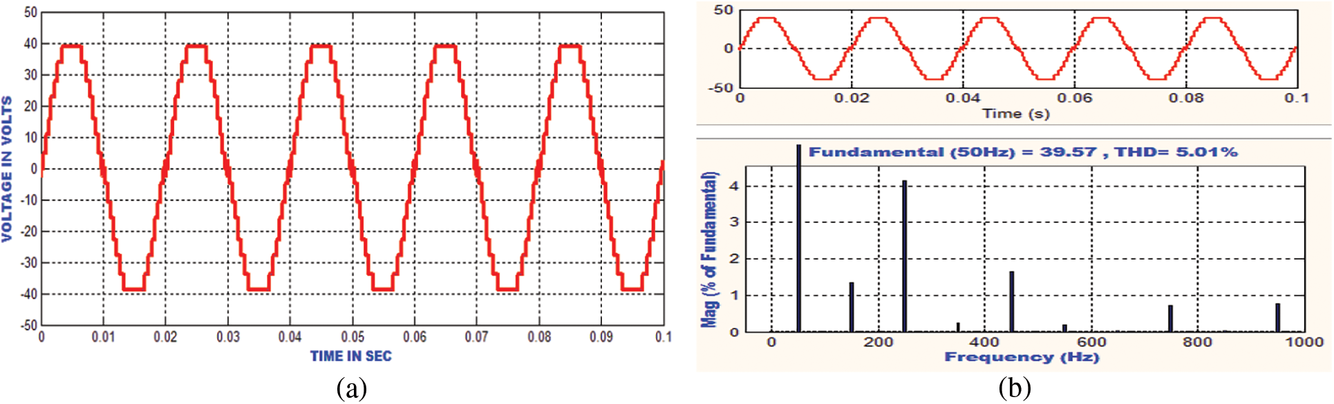
Figure 13: (a): Simulated voltage of fifteen-level inverter using PSO method (b): Simulated THD results of fifteen-level inverter using PSO technique

Then, using THD measurement, the efficacy of the suggested ABC-based selective harmonic elimination method is evaluated. The selected cycles from the MLI output voltage can be used to measure THD. Figs. 14a and 14b show the proposed method used in the MLI and the complying THD (b). The proposed ABC approach has a THD level of 4.86%, which is better than the other two standard methods. By relating the available methods the proposed method is providing a better THD level and adequate presentation for the load. The proposed method can produce required waveforms with a widespread range of modulation indices and diminished THD for the voltage.

Figure 14: (a): Simulated voltage of fifteen-level inverter using ABC based SHE method (b): ABC-SHE technique based 15 level inverter result

Tab. 4 compares the different duty cycle vs. voltage conversion ratios of various converters namely sepic, cuk, boost and buck-boost converters. From the above comparison, the sepic converter achieves a high voltage conversion ratio.

To validate the system’s performance, Tab. 5 compares the proposed topology scheme to certain extant topologies. The number of power semiconductor switches employed in the system is the starting point for this comparison. A circuit’s number of switching devices is an important issue. This component is important since switching losses, driving circuits, and size cost-effectiveness is all closely connected.

When the smallest number of switches are employed for the same level, switching losses are decreased. The size of the driving circuits is only determined by the number of switching devices employed, resulting in a smaller overall circuit. The system’s efficiency is also improved at the same time. Only Fifteen levels are provided in this work.

The existing topologies such as DC15LI, FC15LI, and CHB15LI utilize 28 switching devices, and more DC bus capacitors to achieve the 15 level inverter. When compared to existing topologies, the proposed system uses only 3 DC sources and 8 switches for the same 15 levels. As a result, when compared to current systems, the suggested model employs the fewest switches for the same output levels. As a result, the proposed module is more compact than previous designs. Switching losses are decreased as a result, and overall performance is improved.

6  Conclusion

Selective Harmonics Elimination PWM based on the ABC, PSO, and FPA algorithms is used to reduce the lower order symphonious. Using a high gain dc to constant current SEPIC converter, the Grey Wolf Optimizer harvests the majority of the power from the PV system. Multi-carrier modulation is used to create and assess the suggested reduced switch fifteen-level inverter. Finally, the ABC-SHE methodology achieves less harmonic content than the other three procedures, is contrasted to approaches as well as high-frequency modulation techniques but it is Slow when in sequential processing, so in the future use of the Artificial neural network method to overcome the drawbacks of ABC.

Funding Statement: The authors received no specific funding for this study.

Conflicts of Interest: The authors declare that they have no conflicts of interest to report regarding the present study.

References

 1.  M. Ahmed and E. Hendawi, “A new single-phase asymmetrical cascaded multileveldc-link inverter,” Journal of Power Electronics, vol. 16, no. 4, pp. 1504–1512, 2016. [Google Scholar]

 2.  N. A Rahim, K. Chaniago, J. Selvaraj, “Single-Phase Seven-Level Grid-Connected Inverter for Photovoltaic System,” IEEE Trans. Ind. Electron, vol. 58, no. 6, pp. 2435–2443, 2011. [Google Scholar]

 3.  S. Ganapathy, “An improved artificial bee colony algorithm based harmonic control for multilevel inverter,” Journal of Control Engineering and Applied Informatics, vol. 21, no. 4, pp. 59–70, 2019. [Google Scholar]

 4.  A. Ajami, M. R. J. Oskuee, A. Mokhberdoran and A. V. D. Bossche, “Developed cascaded multilevel invertertopology to minimise the number of circuit devices and voltage stresses of switches,” IET Power Electronics, vol. 7, no. 2, pp. 459–466, 2013. [Google Scholar]

 5.  M. S. Dahidah and V. G. Agelidis, “Selective harmonic elimination pwm control for cascaded multilevel voltage source converters: A generalized formula,” IEEE Transactions on power electronics, vol. 23, no. 4, pp. 1620–1630, 2008. [Google Scholar]

 6.  E. Villanueva, P. Correa, J. Rodriguez, and M. Pacas, “Control of asingle-phase cascaded H-bridge multilevel inverter for grid-connectedphotovoltaic systems,” IEEE Transactions on Industrial Electronics, vol. 56, no. 11, pp. 4399–4406, 2009. [Google Scholar]

 7.  N. A. Rahim, K. Chaniago, J. Selvaraj, “Single-Phase Seven-Level Grid-Connected Inverter for Photovoltaic System,” IEEE Trans. Ind. Electron, vol. 58, no. 6, pp. 2435–2443, 2011. [Google Scholar]

 8.  A. Kasprowicz, “Induction generator with three-level inverters and LCL filter connected to the power grid,” Bulletin of the Polish Academy of Sciences: Technical Sciences, vol. 67, no. 3, pp. 593–604, 2019. [Google Scholar]

 9.  J. Jeyashanthi and J. B. Banu, “ANN-based direct torque control Scheme of an IM Drive for a wide range of speed operation,” Neural Network World, vol. 31, no. 6, pp. 395–414. 2021. https://doi.org/10.14311/NNW.2021.31.022. [Google Scholar]

10. J. Espinoza, G. Joós and J. Guzmán, “Selective harmonic elimination and current/voltage control in current/voltage source topologies: A unified approach,” IEEE Trans Ind Electron, vol. 48, pp. 71–81, 2001. [Google Scholar]

11. M. S. Dahidah, G. Konstantinou and V. G. Agelidis, “A review of multilevel selective harmonic elimination pwm: Formulations, solving algorithms, implementation and applications,” IEEE Transactions on Power Electronics, vol. 30, no. 8, pp. 4091–4106, 2014. [Google Scholar]

12. M. A. Memon, S. Mekhilef, M. Mubin and M. Aamir, “Selective harmonic elimination in inverters using bio-inspired intelligent algorithms for renewable energy conversion applications: A review,“ Renewable and Sustainable Energy Reviews, vol. 82, pp. 2235–2253, 2018. [Google Scholar]

13. S. S. Lee, B. Chu, N. R. N. Idris, H. H. Goh, and Y. E. Heng, “Switched-Battery Boost-Multilevel Inverter with GA Optimized SHEPWM for Standalone Application,” IEEE Transactions on Industrial Electronics, vol. 63, no. 4, pp. 2133–2142, 2016. [Google Scholar]

14. H. Z. Maia, T. H. Mateus, B. Ozpineci, L. M. Tolbert and J. O. Pinto, “Adaptive selective harmonic minimization based on anns for cascade multilevel inverters with varying dc sources,” IEEE Transactions on Industrial Electronics, vol. 60, no. 5, pp. 1955–1962, 2012. [Google Scholar]

15. S. Kundu, A. D. Burman., S. K. Giri, S. Mukherjee and S. Banerjee, “Comparative study between different optimization techniques for finding precise switching angle for SHE-PWM of three phase seven-level cascaded H-bridge inverter,” IET Power Electronics, vol. 11, no. 3, pp. 600–609, 2018. [Google Scholar]

16. J. B. Banu and J. Jeyashanthi. “DTC-IM drive using adaptive neuro fuzzy inference strategy with multilevel inverter,” Journal of Ambient Intelligence and Humanized Computing, pp. 1–23. on line published. https://doi.org/10.1007/s12652-021-03244-3. [Google Scholar]

17. M. B. Satti and A. Hasan, “Direct model predictive control of novel h-bridge multilevel inverter based grid-connected photovoltaic system,” IEEE Access, vol. 7, pp. 62750–62758, 2019. [Google Scholar]

18. S. Kundu, A. D. Burman, S. K. Giri et al., “Comparative study between different optimisation techniques for finding precise switching angle for SHE-PWM of three-phase sevenlevel cascaded H-bridge inverter,” IET Power Electron, vol. 11, no. 3, pp. 600–609, 2017. [Google Scholar]

19. A. Routray, R. K. Singh and R. Mahanty, “Harmonic minimization in three-phase hybrid cascaded multilevel inverter using modified particle swarm optimization,” IEEE Trans Ind Inf., vol. 15, no. 8, pp. 4407–4417, 2018. [Google Scholar]