
 Submit a Paper
 Propose a Special lssue
 Open Access
ARTICLE

Evaluation of Grid-Connected Photovoltaic Plants Based on Clustering Methods
Computer Engineering Department, Umm Al-Qura University, Saudi Arabia
* Corresponding Author: Amr A. Munshi. Email:
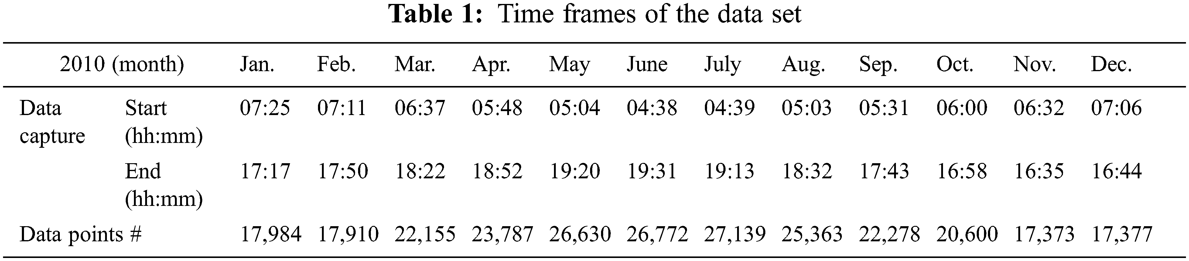
Computer Systems Science and Engineering 2023, 45(3), 2837-2852. https://doi.org/10.32604/csse.2023.033168
Received 09 June 2022; Accepted 18 August 2022; Issue published 21 December 2022
 View Full Text
 Download PDF
Abstract
Photovoltaic (PV) systems are electric power systems designed to supply usable solar power by means of photovoltaics, which is the conversion of light into electricity using semiconducting materials. PV systems have gained much attention and are a very attractive energy resource nowadays. The substantial advantage of PV systems is the usage of the most abundant and free energy from the sun. PV systems play an important role in reducing feeder losses, improving voltage profiles and providing ancillary services to local loads. However, large PV grid-connected systems may have a destructive impact on the stability of the electric grid. This is due to the fluctuations of the output AC power generated from the PV systems according to the variations in the solar energy levels. Thus, the electrical distribution system with high penetration of PV systems is subject to performance degradation and instabilities. For that, this project attempts to enhance the integration process of PV systems into electrical grids by analyzing the impact of installing grid-connected PV plants. To accomplish this, an indicative representation of solar irradiation datasets is used for planning and power flow studies of the electric network prior to PV systems installation. Those datasets contain lengthy historical observations of solar energy data, that requires extensive analysis and simulations. To overcome that the lengthy historical datasets are reduced and clustered while preserving the original data characteristics. The resultant clusters can be utilized in the planning stage and simulation studies. Accordingly, studies related to PV systems integration into the electric grid are conducted in an efficient manner, avoiding computing resources and processing times with easier and practical implementation.Keywords
Photovoltaic (PV) systems are a promising solution to overcome problems associated with the generation of electricity from fossil fuels and the corresponding environmental pollution. While the deployment volume of solar power was limited due to COVID-19 and the silicon raw material shortage in 2021, major PV solar markets and new silicon factories coming online will result in additions of over 200 GW per year as of 2022. It is expected that the global cumulative PV solar capacity will nearly reach 1.9 TW by the year 2025 [1]. Despite the continuous increased dependence on PV systems, there exist numerous challenges that limit the high penetration of these clean resources into the electrical grid. PV systems incorporate negative impacts upon the generation, transmission and distribution system. The major challenge in the generation system is the possibility of spinning reserve requirements. From the transmission side, PV systems may induce voltage profile problems, stability problems and power flow fluctuations. Further, PV systems significantly influence the distribution system with negative impacts, including power fluctuations, voltage sags, power loss in feeders, protection problems and resonance between PV system filtering components and the remaining parts of the distribution network. These challenges could be approached and investigated by thorough analysis of the impact of PV systems on the electrical grid at the design phase prior to their installation. The impact of PV systems on the electrical grid could be investigated through three main approaches:
– Deterministic approach: that considers certain values of PV generation and loading conditions of the network. This method is simple but yields non accurate results. It is mainly used to provide an overview of the expected performance of the electric system under specific operating conditions.
– Probabilistic approach: that treats the output of the PV system and the loading conditions as random variables obtained by appropriate probability density functions. This approach yields better results as compared to the deterministic approach.
– Chronological simulations approach: computer-based simulations utilize time series date of solar irradiance to compute the actual generated AC PV power. The amount of generated PV power is analyzed through a simulation model according to the actual loading conditions and electrical grid parameters. This method is considered appropriate; however, the main drawback is the associated computational complexity and sophisticated hardware requirements.
Rigorous research effort has been devoted to cluster power patterns and obtain cluster representatives during the last few years. Models to group electrical load patterns of customers to assist in tariff formation based on machine learning and clustering techniques were presented in [2–10], short-term forecasting purposes [11] and in demand response programs for support management applications [12–14]. In [15], aggregate modeling of wind farms was proposed based on the wind farm layout and clustering of wind speed data. A method to improve the management decisions of wind farms was also proposed in [6] by applying a clustering method on wind power loads. PV power clustering has become an active area of research for analyzing the output power fluctuation effects on integrating PV systems into the electrical grid [16] and for determining the optimal location and size of PV plants [17]. The potential of PV in becoming a major power resource world-wide [18] motivates the investigation of applying various clustering techniques to investigate the most appropriate technique for clustering PV power.
This paper presents a simplified approach that can be used with chronological simulations to investigate the impacts of PV systems on the electrical grid. Lengthy historical observations of solar irradiance data sets are captured and retreated to estimate the injected AC power from the PV system to the electrical grid. Any fluctuations in the PV power will be reflected on the estimated AC power. The estimated AC PV powers are then regrouped into clusters that contain similar features using different clustering methods such as, k-means and hierarchical clustering algorithms. Therefore, the high dimension data set with correlated feature vectors are reduced. Moreover, the estimated data set (AC PV power) is subjected to dimensionality reduction to reduce the computational complexity while retaining the useful information using principal component analysis (PCA) technique [19]. This enables to conduct PV related simulations with reduced burden, accordingly, integrate PV systems into the electrical grid. Further, the outcome of this approach could be extended to study the possible solutions that can be adopted to reduce the negative impacts of installing grid-connected PV systems by selecting the appropriate penetration level of the PV system for specific distribution system, selecting suitable location for installing the PV system, and study the economic impact of operating the PV system below the rated power in case of reduced solar irradiance.
The data set under study is obtained from Solar Radiation Research Laboratory [20] and includes the global horizontal irradiation (
2.2 Estimated Injected PV Power to the Electrical Grid
The solar irradiation levels obtained from the data set are converted into the equivalent injected AC power to the electrical grid. The equivalent AC power is obtained through the following steps:
• Calculation of tilted irradiation
The solar irradiation data are measured on the horizontal surfaces. Usually, the PV panels are tilted from the horizontal surface by a prespecified angle for maximum power tracking. The global irradiance on the tilted surface can be computed from [21]:
where
The global irradiance on the tilted surface (
where
The direct irradiance on tilted surface (
where
The zenith angle (
where
From Eqs. (4)–(6), all solar angles can be computed and used in Eq. (3) to obtain the tilted global irradiance (
The reflected irradiance (
where
Using Eqs. (3) and (7), the tilted irradiance is obtained from the raw data set.
• Calculation of DC Output Power of the PV Panel
The global irradiance on the tilted surface is used to estimate the equivalent output DC power from the PV array. The output DC power (Pdc) can be estimated according to:
where
• Calculation of AC Output Power of the PV Panel
The final calculation step is to estimate the total amount of injected PV AC power to the electrical grid. The injected AC power is computed from:
where
Clustering techniques are applied to group feature vectors that have similar features to each category of the year. Then representatives from each cluster of the equivalent output AC power are obtained. Those cluster representatives can be used to evaluate the electric network performance in the planning stage prior to PV systems installations instead of using the numerous data points in the raw data set. Consequently, a representative could be used in the simulation studies instead of all the data.
Clustering algorithms are mainly divided into two categories; partitional and hierarchical. In partitional type, data points are grouped into specified and predetermined partitions, such as K-Means clustering algorithm [22]. The main objective of the K-Means algorithm is to minimize the within group sum-of-squares. With predetermined clusters (nc), the algorithm randomly assigns nc centroids. Each data point is assigned to the closest centroid and then the centroids are updated. The assignment and updating process is repeated until there are no more changes to be made. An advantage of the K-Means algorithm is that it only requires the data as input, not the interpoint distance matrix which makes it suitable for large number of data points.
Hierarchical algorithms are categorized into two groups; 1) agglomerative which starts with every data point as a single cluster and then merges them together, and 2) divisive which starts with clustered data points and then splits them (less commonly used). The main concern with this clustering approach is that the number of clusters are not predetermined which may not fit some applications. Dendrograms are yielded from the hierarchical clustering to visually represent the clusters and sub-clusters. Unlike the K-Means algorithm, the proximity among clusters is required in the clustering algorithm. Depending on the measuring tool the clustering behavior is changed. The most common distance measures are: single linkage, complete linkage, average linkage, centroid linkage and Ward’s method. Single and average linkage methods are considered in this work.
In this work, K-Means and agglomerative hierarchical clustering algorithms are applied to the original data set with comparisons. The comparisons are based on one of the cluster evaluation techniques such as the Silhouette Index.
• Silhouette Index
The Silhouette index (SI) [23] evaluates the clustering quality according to the corresponding number of clusters. It can properly provide the suitable number of clusters that should be considered. The average distance between ith observation and all other observations in the same cluster is represented by ai. Besides, the average distance between the ith observation and all other observations not included in the same cluster is bi. The silhouette width for the ith observation
From Eq. (10), the SI, can be found by computing the average of all individual silhouette widths as shown in Eq. (11).
Large silhouette width implies good clustering.
2.4 Representing the AC Power into a Reduced Order Time Series
The considered data set is for the whole year of 2010. Each month in that year is considered separately as an AC power category to form a (m × n) pattern matrix (Xi); where i is from 1 to 12 to representing the year months. It is required to reduce the dimensionality of each pattern matrix using principal component analysis (PCA) [19] technique.
1- For each AC power category (each month in 2010 year), form a (m × n) pattern matrix (Xi) where m is the number the AC power data point with one minute resolution (features) and n represents the index of days in each month (d1, …, d31). As an example, for January month, X1 is formed with (606 × 31) dimensions. Each column of the pattern matrix (d1, …, d31) is considered as a feature vector.
2- Calculate the mean value of each feature vector and subtract that mean from the original feature vector to obtain a new pattern matrix (Zi) with zero mean.
3- Calculate the covariance matrix (cov) of Zi using:
4- Calculate m eigenvalues and m eigenvectors of the covariance matrix (cov).
5- Sort the eigenvector matrix in descending order according to the corresponding eigenvalues. The first eigenvector should correspond to the highest eigenvalue, and so on.
6- Using the eigenvalues and their indices (m), plot the SCREE plot to define the highest L eigenvalues that should be considered. The value of L can be defined by looking at the elbow of the curve or the location where the curve level off (becomes flat).
7- The selected L eigenvectors represent the principal components (PCs). Form a matrix V that contains those PCs with dimension (m × L).
8- Finally, the projection of the original data points onto the new space forms a reduced data set (
9- Evaluate the accuracy of the created reduced matrix using the eigenvalues.
10- The steps 1 → 9 are applied to each AC PV category (each month).
As mentioned, the 2010 year is categorized according to its month. Each month is treated as standalone AC power category. In this section, the month of January is considered for the simulation study. The same methodology can be applied to the remaining months.
The clustering algorithms are applied as follows:
• K-Means Clustering
The K-Means clustering algorithm is applied with k = 5, 10 and 15 clusters as shown in Fig. 1.
• Average Linkage Hierarchical Clustering
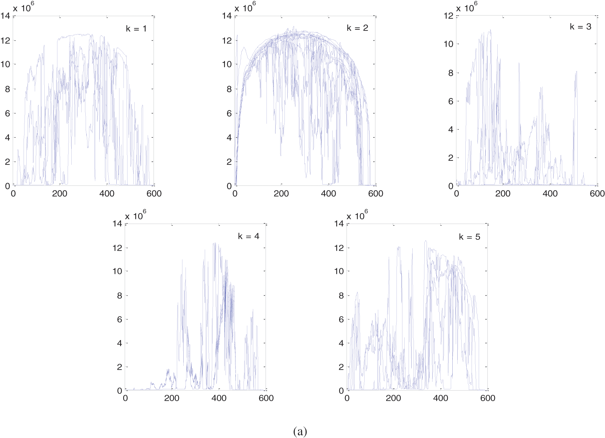
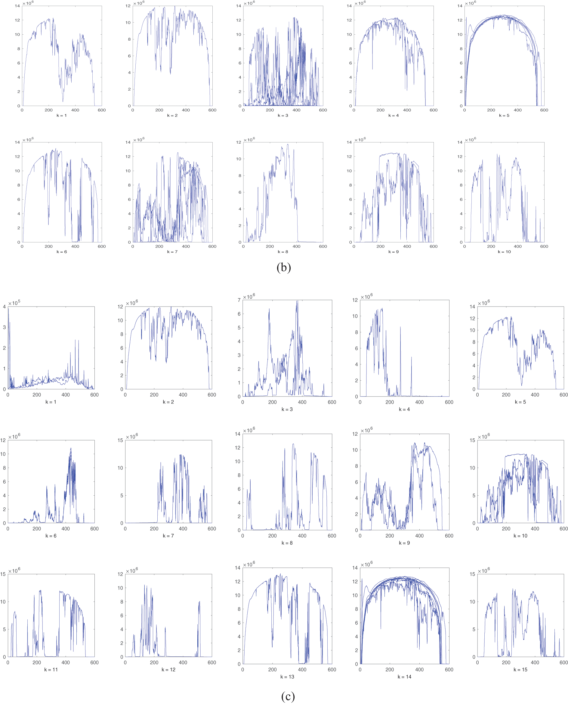
Figure 1: K-Means clusters, (a) 5 clusters. (b) 10 clusters. (c) 15 clusters. Horizontal axis: number of data points (features), vertical axis: generated AC power
The results of applying the average linkage hierarchical cluster is shown in Fig. 2 with the number of clusters set to 5, 10 and 15 clusters.
• Single Linkage Hierarchical Clustering
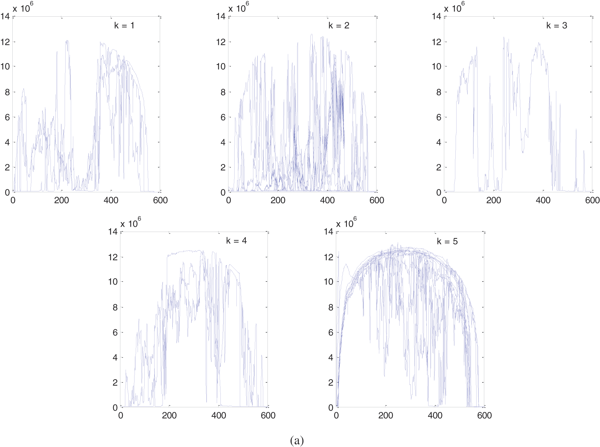
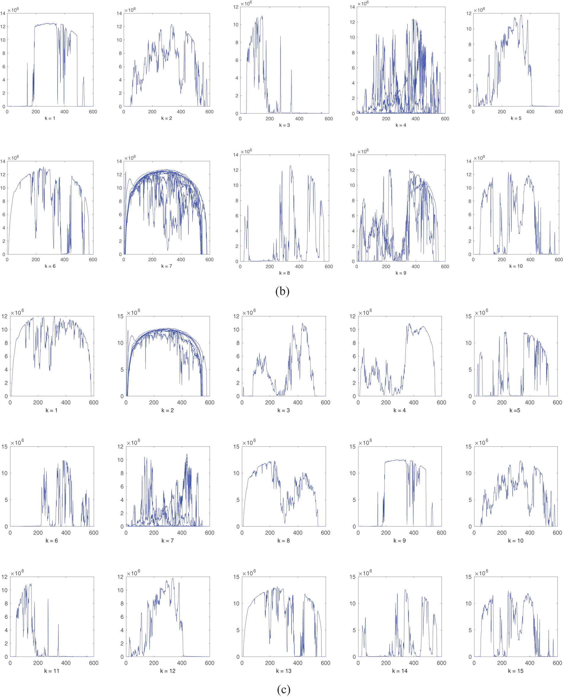
Figure 2: Average linkage hierarchical clusters. (a) 5 clusters. (b) 10 clusters. (c) 15 clusters. Horizontal axis: number of data points (features), vertical axis: generated AC power
The single linkage clustering algorithm is applied with 5, 10 and 15 clusters and the results are shown in Fig. 3.
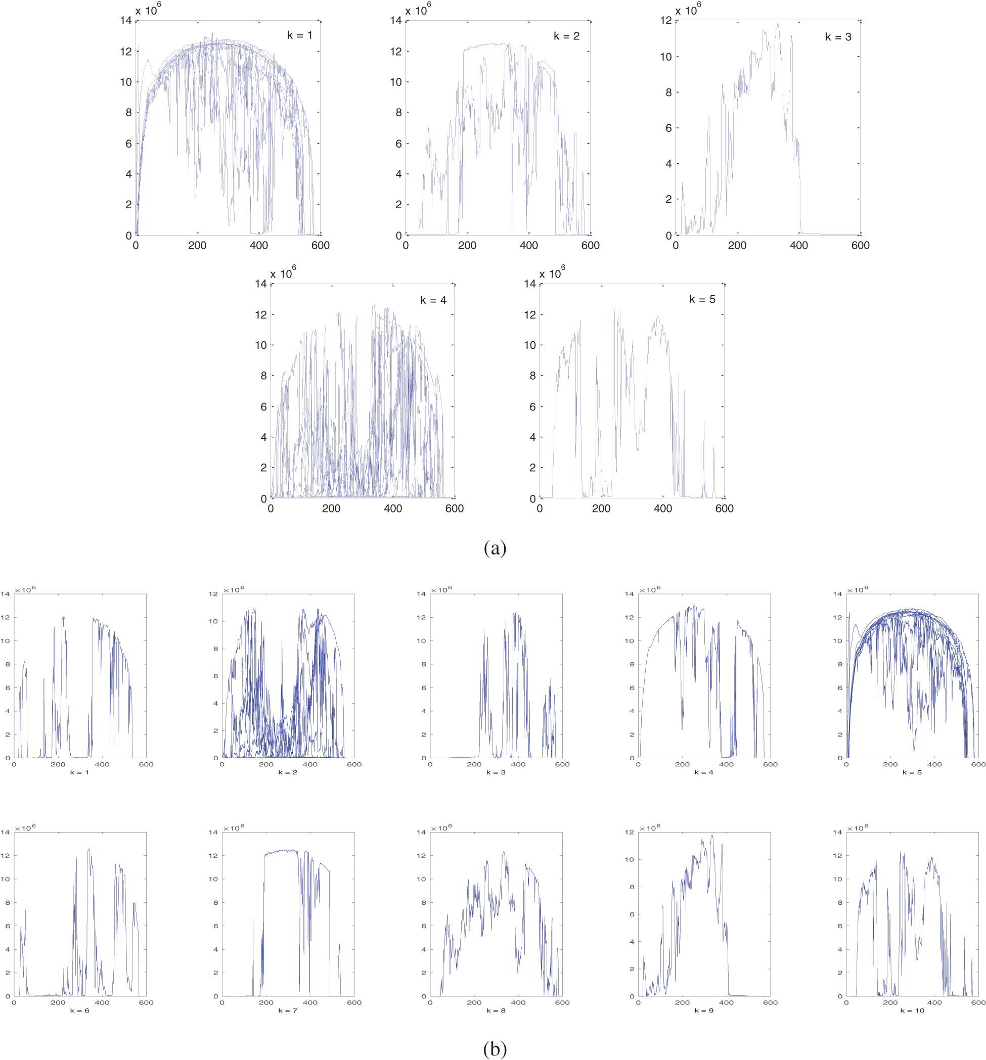
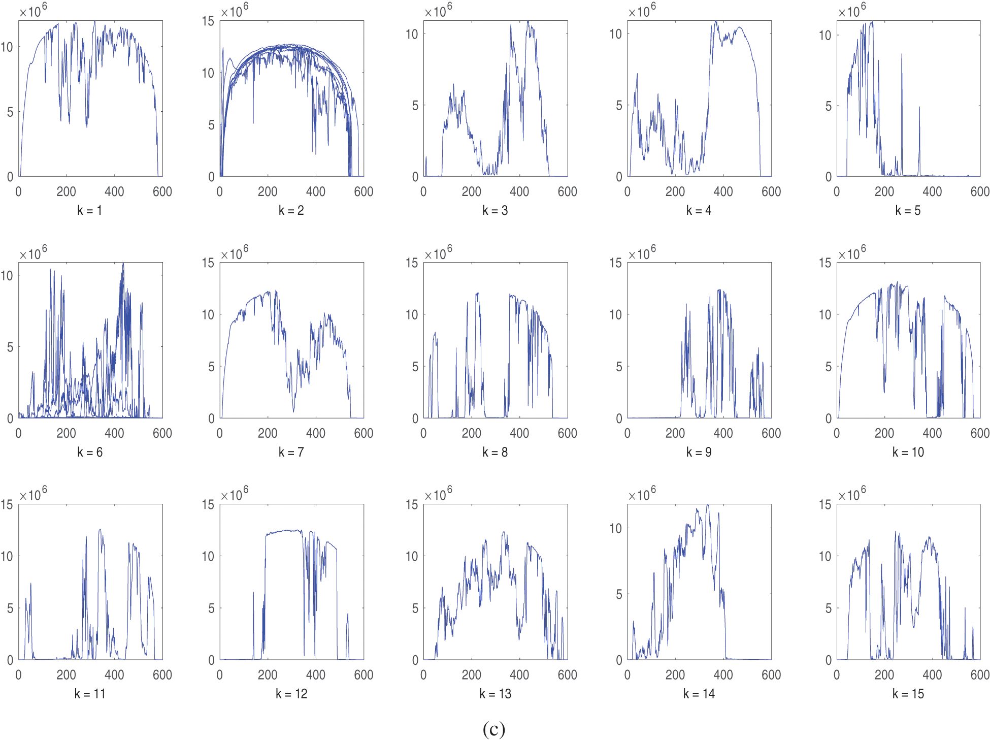
Figure 3: Single linkage hierarchical. (a) 5 clusters. (b) 10 clusters. (c) 15 clusters. Horizontal axis: number of data points (features), vertical axis: generated AC power
The Silhouette index is used to evaluate the results of the cluster algorithms, and the effect of the number of clusters on the SI index shown in Figs. 4 and 5.
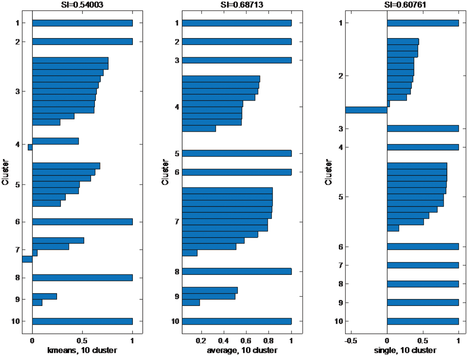
Figure 4: Silhouette index for the three clustering methods for 5 clusters
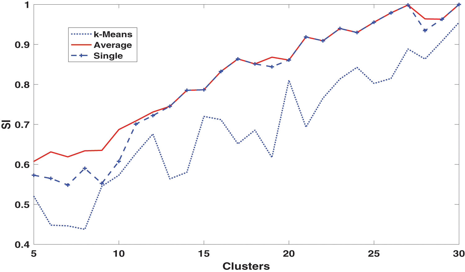
Figure 5: Silhouette index with the increase of the number of clusters
3.3 Reduced Dimension Data Set
• PCA
Applying PCA, the SCREE plot is shown in Fig. 6 for January month AC power category. Fig. 7 shows the accuracy measure of the reduced data set according to the number of PCs.
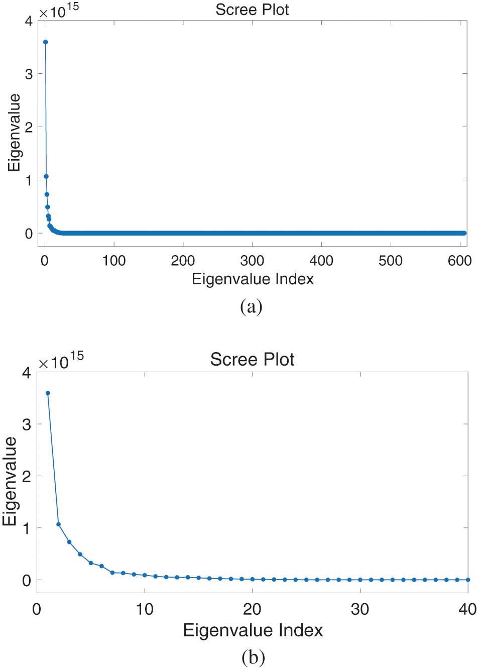
Figure 6: Scree Plot. (a) For the 606 eigenvalue index. (b) Zoomed view
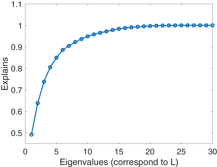
Figure 7: Accuracy measure for the reduced data set (Explains)
• Clustering
Using different clustering techniques, similar feature vectors can be grouped together into clusters to represent the data set in compact format. As shown from Figs. 1–3, the original 31 feature vectors are grouped together into 5 clusters. The methodology can be applied to the remaining categories (each month) in the year of 2010. Note that some clusters have close characteristics while others have some deviations. For instance, clusters produced by K-Means algorithm in Fig. 1 have some deviations in cluster number 1, 3 and 5. The average linkage method, smaller deviations exist in cluster number 2 as compared to K-Means method. The single linkage method has similar trend to the average linkage method with deviated feature vectors in cluster number 4. K-Means clustering is different from hierarchical methods in the sense that it depends on an optimization method to minimize the within-cluster sum-of-square error. On the other hand, the hierarchical methods themselves differ from each other based on the method of computing the distance matrix. As the number of clusters increase, the clustering behavior is improved which is clear from the results in Figs. 1–3 for the same clustering methods with 10 and 15 clusters. From the presented results, it was observed that the average linkage method gives best clusters, and then comes the single linkage method whereas the K-Means clustering method has the weakest cluster formation.
• Silhouette Index
This index is used to determine the number of clusters that can be used according to the resultant clusters quality. Fig. 4 shows silhouette plots for the considered clustering methods with 5 clusters. As shown, each bar in in each cluster represents a feature vector. The length of each bar represents the silhouette width of the corresponding feature vector. The average of all silhouette widths is computed and forms the SI measure. A SI value closer to 1, indicates better clustering formation. Fig. 4 implies that average linkage clustering method has best clustering quality (SI = 0.607) while the K-Means clustering algorithm has the lowest clustering quality (SI = 0.497) which meets the clustered time series in Figs. 1–3.
SI for the considered clustering methods is plotted against different number of clusters as shown in Fig. 5. The maximum number of clusters is the original number of feature vectors (in this case = 31 because it is not feasible to cluster 31 feature vector into 31 + i clusters, i = 1, 2, …). As shown in Fig. 5, SI increases with the increase of number of clusters. At 31st cluster (original data set), SI converges to one (best value of SI) in all methods. However, the number of clusters is required to be as small as possible to reduce the representation dimension of the data set in hand (tradeoff). Similar to previous results, the clustering quality is high with average linkage, then single linkage and low with K-Means method.
4.2 Reduced Dimension Data Set Using PCA
For simulation results on the month of January, the data is organized in a matrix (X1) with columns representing the days of the month and rows representing the AC photovoltaic power for each day with a 1-min time resolution. From the scree plot in Fig. 6b, it can be concluded that selecting 10 eigenvectors as PCs is appropriate. Thus, for the month of January L = 10. Applying the PCA significantly reduces the dimensionality of the data set. The original dimension of the data was 606 × 31, applying the PCA reduced the dimension to 10 × 31. The resultant reduced matrix contains the transformation coefficients which represent the month of January, in this case, to the principal components obtained from the original data set.
The reduced dimension data set accuracy is measured according to the number of PCs considered. As shown in Figs. 7, the PCs 10 and 11 explains 0.9490 and 0.9581 of the original data set, respectively. The number of PCs to be considered as the accuracy measure is subject to the application. In the simulation study, 10 PCs with 0.9490 accuracy measure is considered to reduce the dimensionality as much as possible.
This paper presented an efficient data clustering approach for high dimensional irradiance data set. The estimated PV AC power data set has been categorized into 12 categories for the year of 2010, each representing a month. For instance, January category has been considered with dimension 606 × 31 and has been clustered into 5 distinct clusters. Accordingly, the 31 feature vectors are reduced to 5 by selecting a representative feature vector from each cluster. The Silhouette index was utilized to determine the quality of the resultant clusters according to the selected number of clusters. The average linkage hierarchical clustering method yields the overall best results. The second part of this project introduced PCA method to reduce the dimensionality of the original data set. PCA successfully reduced the dimension from 606 × 31 to 10 × 31 with accuracy measure of 0.949 as compared to the original high dimensional data set. The resultant clusters can be utilized in the planning stage and simulation studies. Accordingly, studies related to PV systems integration into the electric grid are conducted in an efficient manner, avoiding computing resources and processing times with easier and practical implementation. The contributions of the paper to field can be summarized as:
– Comparing between clustering methods from different categories on grouping PV patterns.
– Using validity indices to evaluate the performance of the clustering methods and verify the compactness and separation of the obtained clusters.
– Reducing the dimensionality of photovoltaic power during the clustering process using principal component analysis (PCA).
– Finding the optimum number of clusters for photovoltaic power and presenting a representative power pattern from each cluster that can be used in the simulations and studies of the integration of PV systems into the electrical grid.
Funding Statement: The author received no specific funding for this study.
Conflicts of Interest: The author declares that he has no conflicts of interest to report regarding the present study.
References
1. B. Meban, SolarPower Europe: Global market outlook for solar power 2021–2025, July 2021. [Google Scholar]
2. G. Chicco, R. Napoli, P. Postolache, M. Scutariu and C. Toader, “Customer characterisation options for improving the tariff offer,” IEEE Transactions on Power Systems, vol. 18, no. 1, pp. 381–387, 2003. [Google Scholar]
3. V. Silva, F. Rodrigues, Z. Vale and J. B. Gouveia, “An electric energy consumer characterization framework based on datamining techniques,” IEEE Transactions on Power Systems, vol. 20, no. 2, pp. 596–602, 2005. [Google Scholar]
4. D. Gerbec, S. Gasperic, I. Smon and F. Gubina, “Determining the load profiles of consumers based on fuzzy logic and probability neural networks,” Proceedings of IET Generation Transmission and Distribution, vol. 151, no. 3, pp. 395–400, 2004. [Google Scholar]
5. A. Munshi and Y. A. I. Mohamed, “Extracting and defining flexibility of residential electrical vehicle charging loads,” IEEE Transactions on Industrial Informatics, vol. 14, no. 2, pp. 448–461, 2018. [Google Scholar]
6. M. Ali, I. -S. Ilie, J. V. Milanovic and G. Chicco, “Wind farm model aggregation using probabilistic clustering,” IEEE Transactions on Power Systems, vol. 28, no. 1, pp. 309–316, 2013. [Google Scholar]
7. G. Chicco, R. Napoli and F. Piglione, “Comparisons among clustering techniques for electricity customer classification,” IEEE Transactions on Power Systems, vol. 21, no. 2, pp. 933–940, May 2006. [Google Scholar]
8. S. V. Verdu, M. O. Garcia, C. Senabre, A. G. Marin and F. J. G. Franco, “Classification, filtering, and identification of electrical customer load patterns through the use of self-organizing maps,” IEEE Transactions on Power Systems, vol. 21, no. 4, pp. 1672–1682, 2006. [Google Scholar]
9. H. Sun and R. Grishman, “Lexicalized dependency paths based supervised learning for relation extraction,” Computer Systems Science and Engineering, vol. 43, no. 3, pp. 861–870, 2022. [Google Scholar]
10. H. Sun and R. Grishman, “Employing lexicalized dependency paths for active learning of relation extraction,” Intelligent Automation & Soft Computing, vol. 34, no. 3, pp. 1415–1423, 2022. [Google Scholar]
11. J. Tsekouras, N. D. Hatziargyriou and E. N. Dialynas, “Two-stage pattern recognition of load curves for classification of electricity customers,” IEEE Transactions on Power Systems, vol. 22, no. 3, pp. 1120–1128, 2007. [Google Scholar]
12. G. Chicco, R. Napoli and F. Piglione, “Load pattern clustering for short-term load forecasting of anomalous days,” in Proc. of IEEE PowerTech Conf., Porto, 10–13 Sept. 2001. [Google Scholar]
13. A. Gabaldon, A. Guillamon, M. C. Ruiz, S. Valero, C. Alvarez et al., “Development of a methodology for clustering electricity-price series to improve customer response initiatives,” IET Generation Transmission and Distribution, vol. 4, no. 6, pp. 706–715, 2010. [Google Scholar]
14. G. J. Tsekouras, C. A. Anastasopoulos, F. D. Kanellos, V. T. Kontargyri, I. S. Karanasiou et al., “A demand side management program of vanadium redox energy storage system for an interconnected power system,” in Proc. of Int. Conf. on Energy Planning, Energy Saving, Environmental Education, Corfu Island, Greece, 2008. [Google Scholar]
15. G. Tsamopoulos, N. Giannitsas, F. D. Kanellos and G. J. Tsekouras, “Load estimation for war-ships based on pattern recognition methods,” Journal of Computations and Modeling, vol. 4, no. 1, pp. 207–222, 2014. [Google Scholar]
16. A. Munshi and Y. Mohamed, “Photovoltaic power pattern clustering based on conventional and swarm clustering methods,” Solar Energy, vol. 124, pp. 39–56, 2016. [Google Scholar]
17. N. Haghdadi, B. Asaei and Z. Gandomkar, “Clustering-based optimal sizing and siting of photovoltaic power plant in distribution network,” in Proc. of Int. Conf. on Environment and Electrical Engineering (EEEIC), Venice, Italy, pp. 266–271, 18–25 May 2012. [Google Scholar]
18. A. Munshi and Y. Mohamed, “Comparisons among Bat algorithms with various objective functions on grouping photovoltaic power patterns,” Solar Energy, vol. 144, pp. 254–266, 2017. [Google Scholar]
19. T. Jolliffe, Principal Component Analysis. 2nd ed., New York: Springer-Verlag, Incorporate, 2002. [Google Scholar]
20. Solar Radiation Research Laboratory (BMS). [Online]. Available: http://www.nrel.gov/midc/srrl_bms, 2020. [Google Scholar]
21. J. Olmo, J. Vida, I. Foyo, Y. C. Diez and L. A. Arboledas, “Prediction of global irradiance on inclined surfaces from horizontal global irradiance,” Elsevier Science, pp. 689–704, 1999. [Google Scholar]
22. D. Hand, H. Manilla and P. Smyth, Principles of Data Mining. Cambridge, MA: MIT Press, 2001. [Google Scholar]
23. R. Jain and R. Koronios, “Innovation in the cluster validating techniques,” Fuzzy Optimization and Decision Making, vol. 7, no. 3, pp. 233–241, 2008. [Google Scholar]
Cite This Article
 Copyright © 2023 The Author(s). Published by Tech Science Press.
This work is licensed under a Creative Commons Attribution 4.0 International License , which permits unrestricted use, distribution, and reproduction in any medium, provided the original work is properly cited.
 Downloads
 Citation Tools