Hybrid Multi-Strategy Aquila Optimization with Deep Learning Driven Crop Type Classification on Hyperspectral Images

1  Introduction

Agriculture is the foundation of the national economy, and crop productivity will affect the day-to-day lives of humans. Particularly, gaining crops’ spatial distribution and growth status becomes vital for policy development and agriculture monitoring [1]. But the conventional field measurement, investigation, and statistical techniques were labour-intensive and time-consuming, makes tougher to gain agriculture data of a wide area within time. With the advancement of the earth observation technique, the remote sensing (RS) method was broadly implemented in the agricultural sector for years since it could reach a wide area of agricultural land with lower costs and high data collection frequency [2]. A precise and prompt grasp of the data regarding agricultural resources is very significant for the growth of agriculture. Procurement of the spatial distribution and area of crops was an imperative way of gaining agricultural data [3]. Conventional approaches acquire crop classification outcomes by statistics, field measurement, and investigation, which are money-consuming, time-taking, and labour-intensive. Leaps and bounds will advance remote sensing technology, and the timeliness and resolution of remote sensing images (RSI) were enhanced, and HSIs were utilized widely [4]. To be specific, HSI had a crucial role in agricultural surveys and was utilized for agricultural yield estimation, pest monitoring, crop condition monitoring, etc. In agricultural surveys, the HSI’s optimal categorization offers crop distribution data. Fine categorization of crops needs images with higher spectral and spatial resolutions [5]. Recently, airborne HSI technology was advanced rapidly, and the implementation of airborne HSI could resolve the requirements above.

HSI has obtained significance due to developments in RSI acquisition systems and the rising obtainability of rich spectral and spatial information by utilizing different sensors [6]. HSI categorization is becoming important for practical applications in domains like mineral mapping, agriculture, forestry, environment, etc. HSI could gain spectral features and variances more meticulously and comprehensively than panchromatic remote sensing [7]. Thus, this paper will use HSI approaches to optimally categorize crops and promote the advancement of particular applications of HSI methods in agriculture, like monitoring agriculture growth and maximizing agriculture sector management [8]. Several techniques have been implemented for HSI categorization in recent times. Early-stage classifier techniques include random forest (RF), support vector machine (SVM), decision tree, and multiple logistic regression (LR), which could offer promising classifier outcomes [9]. These classification techniques could derive the shallow feature data of HSI, which have a capacity constraint for managing the extremely non-linear HSI dataset and restricts the further development of their classifier accuracy [10]. In recent times, DL-related techniques have also been extended to HSI classification.

This article designs a Hybrid Multi-Strategy Aquila Optimization with a Deep Learning-Driven Crop Type Classification (HMAODL-CTC) algorithm on HSI. The proposed HMAODL-CTC model initially carries out image preprocessing to improve image quality. In addition, the presented HMAODL-CTC model develops dilated convolutional neural network (CNN) for feature extraction. For hyperparameter tuning of the dilated CNN model, the HMAO algorithm is utilized. Eventually, the presented HMAODL-CTC model uses an extreme learning machine (ELM) model for crop type classification. A comprehensive set of simulations were performed to illustrate the enhanced performance of the presented HMAODL-CTC algorithm.

The rest of the paper is organized as follows. Section 2 provides the literature review, and Section 3 offers the proposed model. Later, Section 4 depicts the result analysis, and Section 5 concludes the work.

2  Literature Review

Hamza et al. [11] examine a new squirrel search optimized with deep transfer learning (DTL)-assisted crop classification (SSODTL-CC) technique on HSI. The presented approach appropriately recognizes the crop types from HSI. To achieve this, the study primarily develops MobileNet with Adam optimizing to extract feature procedures. Besides, the SSO approach with the BiLSTM technique was utilized for crop-type classifiers. Meng et al. [12] concentrated on DL-related crop mapping employing one-shot HSI, in which 3 CNN algorithms, 1D-CNN, 2D-CNN, and 3D-CNN techniques, have been used for end-to-end crop maps. Bhosle et al. [13] inspect the employ of DL-CNN for overcoming the problems rising in crop detection with satellite images. EO-1 Hyperion HSIs detect mulberry, cotton, and sugarcane crops during the existing works. DL-CNN was related to deep feedforward neural networks (FFNN).

In [14], the morphological outlines, GLCM texture, and end member abundance features were leveraged for developing the spatial information of HISs. Several spatial data have been fused with novel spectral data for producing classified outcomes by utilizing the DNN with conditional random field (DNN-CRF) technique. With a conditional system, the CRF assumes spatial or contextual data to reduce misclassification noise but retain the object boundary. Gutierrez et al. [15] establish an Intelligent Sine Cosine Optimization with DTL depending on the Crop Type Classification (ISCO-DTLCTC) technique. The proposed approach contains the primary preprocessed step for extracting the ROI. The information gain-related feature reduction method was utilized for reducing the dimensionality of novel HISs. Besides, a fusion of 3 deep CNNs techniques, such as SqueezeNet, Dense-EfficientNet, and VGG16, carry out the extraction feature method. Moreover, the SCO technique with Modified Elman Neural Network (MENN) approach was executed to crop type classifier.

A precise crop classifier approach utilizing spectral-spatial-location fusion dependent upon CRFs (SSLF-CRF) for UAV-borne HSI was presented in [16]. The presented approach combines the spatial feature, spectral data, spatial location, and spatial context data from the CRF technique with probabilistic potentials, offering complementary data to crop discrimination in several views. Wu et al. [17] presented 2 novel classifier structures that are both created in MLPs. Primarily, the authors present a dilation-based MLP (DMLP) technique, where the expanded convolution layer exchanges the conventional convolutional MLP, increasing the receptive field without loss of resolution and maintaining the relative spatial location of the pixel unmodified. Secondarily, the work presents DMLP and multi-branch remaining block regarding efficiency feature fusion, then PCA is named DMLPFFN, creating complete utilization of multi-level feature data of HSIs.

3  The Proposed Model

This article has developed a new HMAODL-CTC technique to classify crops on HSI. The presented HMAODL-CTC technique mainly intends to categorize different types of crops on HSI. The presented HMAODL-CTC technique comprises various processes such as image preprocessing, dilated CNN-based feature extraction, HMAO-based parameter tuning, and ELM classification. Fig. 1 illustrates the block diagram of the HMAODL-CTC system.

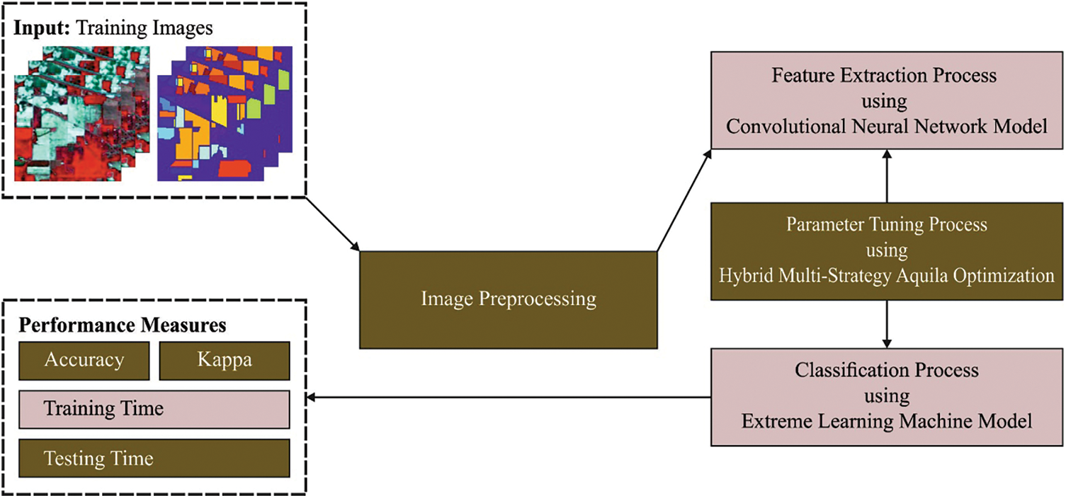
Figure 1: Block diagram of HMAODL-CTC system

3.1 Stage I: Image Preprocessing

Initially, the presented HMAODL-CTC model carries out image preprocessing to improve image quality. Gaussian filtering (GF) is an approach that diminishes pixel variance through weighted averages for image smoothing from various applications [18]. On the other hand, the lower pass filter couldn’t retain image details, for instance, textures and edges. Next, the f linear transformation variant function determines the filtering above method in the following:

f(p)=∑qKp,q(Q)Pq,(1)

Now, Kp,q indicates the q pixel centered at the p pixel in filter kernels K, Q and P correspondingly denotes guidance and input images:

Kp,q(Q)=1nexp⁡(−‖p−q‖2σs2)⋅exp⁡(−‖Pp−Qq‖2σr2),(2)

The exponential distribution function is employed to evaluate the impact of spatial distance usingexp⁡(−‖p−q‖2σr2), and exp⁡(−‖Pp−Qq‖2σr2) defines the effect of pixel intensity range. Eq. (2) simplifies the single image smoothing form if Q and P are similar.

3.2 Stage II: Feature Extraction

At this stage, the presented HMAODL-CTC model applied dilated CNN model for feature extraction. The multiple hidden layers allow the model to efficiently learn the discriminative feature in Dilated CNN network [19]. It empowers the computer to understand complex ideas by making them out of small complexes. The output of the various levels of dilated CNN and attention layers are accountable for feature selection and extraction. The dilated convolution layer’s deep depth attempts to discover granular quality, a hierarchical feature utilized to describe compositional feature data. The feature results are pooled and distributed to the dilated CNN for producing DCV output, different from standard CNN that instantly implements dilated convolutional operations. Every green colored dot shows that these blocks are where chosen convolution is implemented. Consequently, the deep CNN layer produces the subsequent set of parameters as follows:

dcvi=dconv1,dconv2,…,dconvn∈Rn×d∼(3)

Now, d represents the input sequence, and dcv denotes the output of dilated convolution as follows.

DCVl=[dcv1l,dcv2l,…,rvnl]∈Rn∗d∼,l∈(1,L)(4)

L shows the overall convolution box from the expression, and the block filter has a degree of k in the following.

Wl∈Rk∗w∗k,Wl∈Rk∗w∗d∼(5)

Such filtering matrixes W apply that the process held in k time, along with weight w vector. The two neighboring blocks are transformed into

DCV=F(W1,DCVl−1)(6)

It is a sliding of filtering with a window utilized to w-length input, where by f indicates linear algebra formula.

dcvtl=ReLU(Wl⊕[dcvt+1rl−1]t=0w−1)(7)

Now, ⊕ represents convolution, and r indicates the levels of the deep layer in the dilation. The ReLU with every block has the length of (w−1)2L−1. A deep convolutional layer increases exponentially instead of the parameter’s increasing weight. Lastly, hierarchical maps of DCV1, DCV2, ……, and DCVl are attained according to the coupling coefficient relationship on the upstream and downstream layers. SoftMax provides the value of the bio set. Presently, DCV1=[dcv1l,dcv2l,…,dcvnl]∈ Rn∗k∼, l∈(1,L). The l−th convolution block output is now represented as Rn∗k∼, l∈(1,L). Every k filter operation output is produced as COVio′s value utilized as the final output feature. Then, attain COV1=[COV1l,COV2l,…,COVnl]∈RM∗dV. The convolutional term size represents dv, and M shows the quantity of the last convolution. Here, execute the routing DC Vl to CO Vl for information generation and last feature extraction. The prediction vector dcvj∖l^ shows the transformation of raw vector feature viz., evaluated as the multiplication of devi with Wj.

dcv^J∖l=dcvj∗Wj(8)

By decreasing large vectors and raising smaller vectors into unit vectors, these approaches increase the efficacy of data exchange in the complex routing system. An iteratively layered routing method is applied to calculate the medium step over a multi-layered dilated convolutional layer. Fig. 2 displays the architecture of CNN.

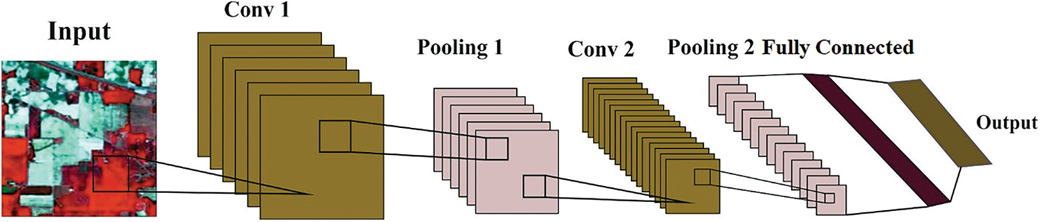
Figure 2: Architecture of CNN

Now, the softmax routing function is srfij, and its variation with dcv is set as aij agreement and evaluated as follows.

aij=covi∗dcv^J∖l+srfij(9)

Generally, the dilated convolutional process allows scalable and more efficient convolutional routing. In these phases, the autonomous final convolutional layer is calculated as V1= [COV1l,COV2l,…,COVnl]∈RM∗dV.

COVl=[COVl,COVl,…,COVl](10)

Afterwards the execution, the action would be passed all over the hierarchical layer. Extracted feature [COVl,COVl,…,COVl] of dilated convolutional would be allocated.

3.3 Stage III: Hyperparameter Tuning

For hyperparameter tuning of the dilated CNN model, the HMAO algorithm is utilized. Aquila Optimizer (AO) is a metaheuristic approach, and it is stimulated by the predation behaviors of Aquila [20]. There exist 4 hunting approaches while the Aquila attack several types of prey.

Expanded exploration of the behavior of Aquila higher soar with a vertical stoop is exploited for hunting birds in a fight. They fly higher levels over the ground and explore the search space for better prey regions. When they find the prey, Aquile takes a vertical dive, and it can be mathematically expressed as follows:

X1(t+1)=Xprey(t)×(1−tT)+r1×(XM(t)−Xprey(t))(11)

In Eq. (11), Xprey(t) represents the better solution, and XM signifies the standard location of the candidate. t and T indicate the amount of existing iteration and the maximal iteration count.

Narrowed exploration (X2): The behavior of Aquila contour fight with the shortest glide attack, and it is better suited for breeding grouse, hunting ground squirrels, or sea birds. They fly low around the selected region and apply the shortest glide to attack the prey. The mathematical expression is given below:

X2(t+1)=Xprey(t)×Levy(D)+XR(t)+r2×(y−x)(12)

In Eq. (12), XR(t) specifies a random location of the candidate, Levy (D) indicates the levy fight (LF) distribution function, and D represents the dimension size. It is expressed in the succeeding expression:

{y=r×cos⁡(θ),x=r×sin⁡(θ)r=r3+U×D1,θ=−ω×D1+32π(13)

In Eq. (13), U indicates a constant value equivalent to 0.00565, ω is fixed as 0.005, and D1 denotes an integer number amongst 1 and the dimension size (D).

Expanded exploitation (X3): The nature of Aquila lower fight with slower descent attack. They employ these approaches for hunting slow prey, namely hedgehogs, rattlesnakes, tortoises, and foxes, or prey without escape response. Afterwards, finding the prey, they prepared for landing and attack. This lower fight altitude to get closer to the prey and observes the reaction of prey, and it is mathematically expressed as follows:

X3(l+1)=(Xprey(t)−X(t))×α−r4+((Ub−Lb)×r5+Lb)×δ(14)

In Eq. (14), α and δ indicate exploitation adjustment parameters. Note that the AO is well-performed when they are set to 0.1. UB and LB indicate the upper and lower bounds of the search space.

Narrowed exploitation: Aquila’s nature is to grab prey, generally large prey. Such behaviours are expressed in the following equation:

{X4(t+1)=QF(t)×Xprey(t)−(G1×X(t)×r6)−G2×Levy(D)+r7×G1QF(t)=tG12×r8−1(1−T)2,=2×r9−1,G2=2×(1−tT)(15)

QF(t) indicates the quality function utilized to equilibrium the search strategy. G1 represents different motions of Aquila while tracing prey that is a random value within (−1,1), and G2 represents the fight slope of Aquila that is reduced from 2 to 0.

Still, the AO has specific problems even though it is satisfactory. Especially the AO needs to balance the exploration and exploitation stages. The evolution from exploration to exploitation process is so stiff that it does not match the present situation. Similarly, the LF distribution function cannot assist the AO exploits the particular search space.

To overcome this problem, the escaping energy (E) and exploitation strategy is used from Harris Hawks Optimization (HHO):

E=2×E0×(1−tT)=G1×G2(16)

In Eq. (16), E0 shows a number within (−1,1) in all the iterations. If |E|≥1, they explore to find the prey location. If |E|<1, they begin to exploit the nearby space of prey.

If rand≥0.5, utilize Soft and Hard besiege approaches in HHO as an exploitation strategy. If |E|≥0.5, Aquila gently encircles the prey to consume the prey’s energy and later attack it. Such behaviors are shown below:

{X5(t+1)=△X(t)−E|JXprey(t)−X(t)△X(t)=Xprey(t)−X(t),J=2×(1−r10)(17)

In Eq. (17), △X(t) signifies the difference between Xprey(t) and (t). E represents the escaping energy, J refers to the random jump strength of the prey.

If |E|<0.5, then the prey has slight energy to escape, making the Aquila readily encircle the prey and attack:

X6(t+1)=Xprey(t)−E|△X(t)|(18)

Note that Xprey characterizes the better location attained so far has greater effects on outcomes. Hence, Elite Evolution Strategy (ESS) is intended for enhancing xprey. EES primarily involves two techniques: elite random mutation and elite natural evolution. In ESS, three elite chromosomes are developed for evolution which are E1, E2, and E3. The mathematical expression of the cross-recombination of genes is given below:

X′={E1,r11<spE2,r11>spandr12≥0.5E3,r11>spandr12<0.5sp=rand(−1,1)×(1−tT)(19)

In Eq. (19), X′ characterizes a new E1, E2 and E3. sp control the proportion of E1 in the novel chromosome. Elite random mutation aim is to mutate some genes of E1. It gives E1 further possibilities to escape from local optimal, and it is mathematically expressed in the following equation:

X′={CL+N(μ=0,σ=1)|CL−E1|,r13<spE1,r13>sp(20)

In Eq. (20), CL characterizes the center location vector. N(μ=0,σ=1) indicates a sequence that conforms to Gaussian probability distribution. r1−r13 shows random numbers within (0,1). By using ESS, a novel chromosome X′ is attained. If it is better than the present xprey, replace xprey with X′. For every strategy, utilize a greedy selection model; hence the best location is chosen as the following location for the novel iteration.

3.4 Stage IV: Crop Type Classification

Finally, the presented HMAODL-CTC model uses the ELM model for crop type classification. It is a single hidden unit that could arbitrarily alter and produce hidden layer numbers with these properties; the ELM-based AL technique saves much training time [21]. As an SLNN, compared to other conventional SLFN techniques, ELM could promise to learn accuracy while fast learning speed. ELM applies biases b and weights w. Furthermore, training databases are represented by 𝒟train∈Rl, which is previously encoded using TF-IDF as {X,Y}={{x1,y1}, …, {xj,yi}, …, {χl,yl}}, while χj indicates the instance and yi denotes the ground truth label. g() represents the sigmoid activation function in the (h) hidden layer. Therefore, it is formulated in the following equation:

F(x)=βg(X,w,b)(21)

While β indicates the weighted matrixes, w represents the weight between input and hidden nodes, and b implies the bias. Compared to the normal SLFN, the primary objective of ELM is that the initial parameter in β is randomly produced afterwards, fixing the activation functions and several hidden units as follows:

L(X,Y,β)=‖Y−βH‖2→0(22)

H=g(X,w,b)(23)

From the expression, X indicates the text, Y denotes the true textual emotion labels, and H represents the collection matrix regarding the activation function as follows.

β^=H∗Y,(24)

In Eq. (24), H∗ specifies the Moore-Penrose generalized inverse of H. Additionally, the learned variable β^ plays a primary role in forecasting raw Chinese textual emotion labels. By considering ELM, the study separated its architecture into predicting and learning. During the learning process, the objective is to learn the β^ parameter.

4  Results and Discussion

In this section, the crop type classification results of the HMAODL-CT model are tested using three databases, namely INB [22], UPB [23], and SSB [24]. The parameter settings are as follows: learning rate: 0.01, dropout: 0.5, batch size: 5, stride: 4, epoch count: 50, and activation: ReLU. The CNN model has 2 convolution layers, 2 pooling layers, 2 fully connected, and 1 softmax layer.

Fig. 3 demonstrates the overall crop type classification results of the HMAODL-CT technique on the IND database. These results indicated that the HMAODL-CT system had reached better results in all cases. For example, with 5% of TR data, the HMAODL-CT technique has offered overallaccy,avgaccy, and kappa of 87.67%, 86.03%, and 83.75%, correspondingly. In addition, with 15% of TR data, the HMAODL-CT approach has presented overallaccy,avgaccy, and kappa of 99%, 98.24%, and 97.82%, correspondingly. Also, with 25% of TR data, the HMAODL-CT method has granted overallaccy,avgaccy, and kappa of 99.87%, 99.64%, and 99.45%, correspondingly.

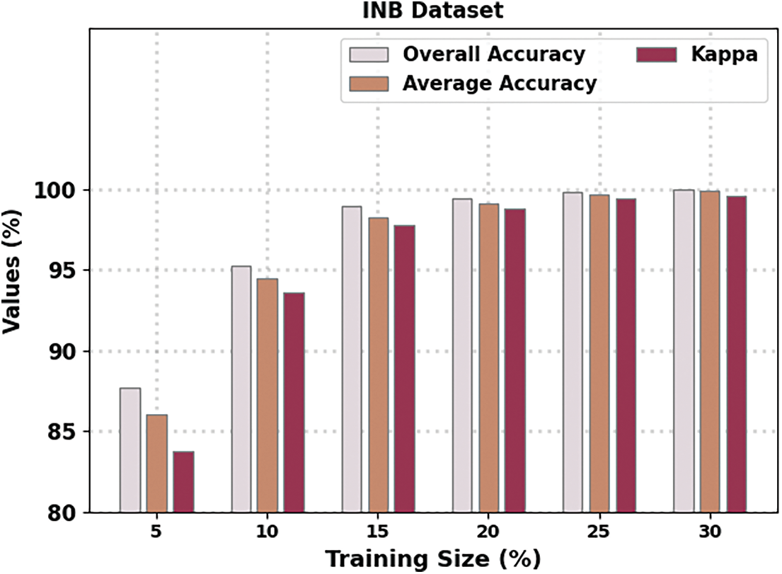
Figure 3: Result analysis of the HMAODL-CT approach under the IND database

Fig. 4 illustrates an overall crop type classification result of the HMAODL-CT methodology on the UPB database. These specified HMAODL-CT approaches have obtained enhanced results in all cases. For example, with 5% of TR data, the HMAODL-CT technique has offered overallaccy,avgaccy, and kappa of 98.47%, 97.77%, and 96.78%, correspondingly. Moreover, with 15% of TR data, the HMAODL-CT technique has presented overallaccy,avgaccy, and kappa of 99.81%, 99.74%, and 99.82%, correspondingly. Also, with 25% of TR data, the HMAODL-CT algorithm has rendered overallaccy,avgaccy, and kappa of 99.97%, 99.91%, and 99.89%, correspondingly.

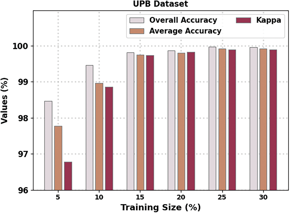
Figure 4: Result analysis of HMAODL-CT approach under UPB database

Fig. 5 portrays an overall crop type classification result of the HMAODL-CT methodology on the SAB database. These results denoted the HMAODL-CT approach has reached enhanced results in all cases. For example, with 5% of TR data, the HMAODL-CT technique has provided overallaccy,avgaccy, and kappa of 99.26%, 99.15%, and 98.93%, correspondingly. Also, with 15% of TR data, the HMAODL-CT technique has shown overallaccy,avgaccy, and kappa of 99.98%, 99.96%, and 99.97%, correspondingly. Also, with 25% of TR data, the HMAODL-CT approach has displayed overallaccy,avgaccy, and kappa of 99.99%, 99.98%, and 99.99%, correspondingly.

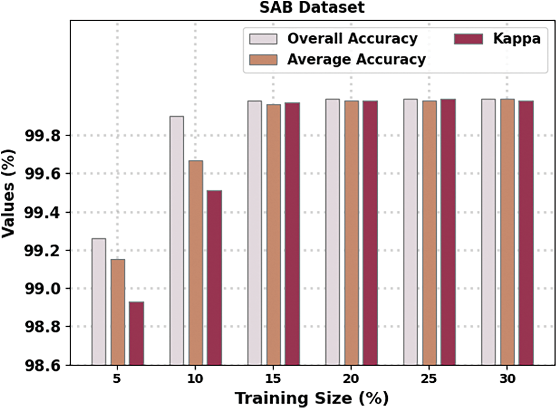
Figure 5: Result analysis of the HMAODL-CT approach under the SAB database

Fig. 6 presents the accuracy and loss graph analysis of the HMAODL-CT method under three databases. The fallouts displayed that the accuracy value tends to rise, and the loss value tends to decline with an increasing epoch count. Note that the training loss is lower, while the validation accuracy is higher in the three databases.

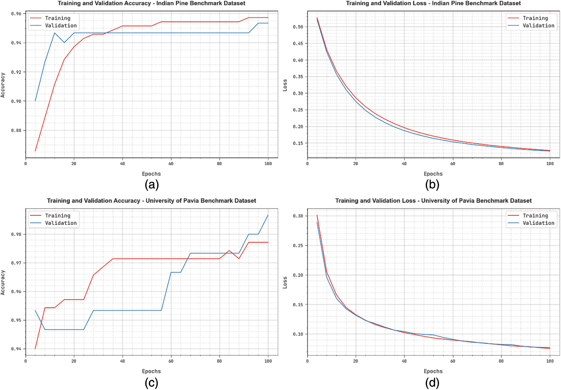
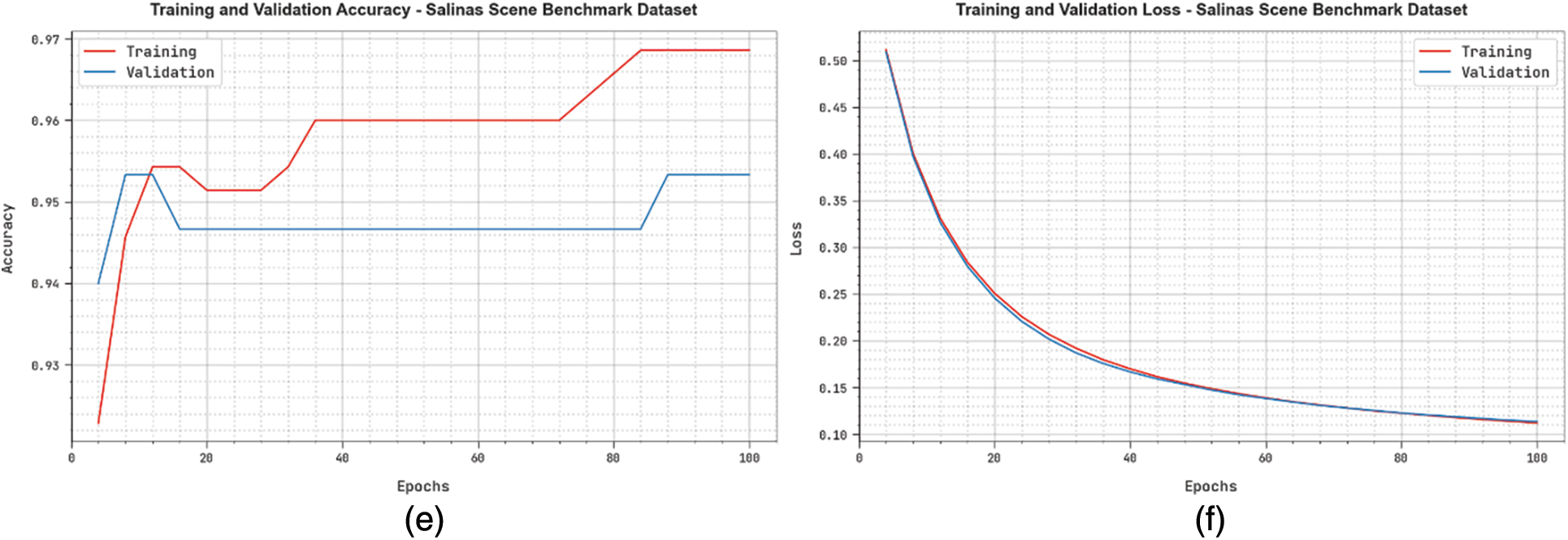
Figure 6: (a and b) Graph of Accuracy and Loss-INB Database (c and d) Graph of Accuracy and Loss-UPB Database (e and f) Graph of Accuracy and Loss-SAB Database

Fig. 7 represents the training time (TRT) examination of the HMAODL-CT technique with the existing HDSRN approach. The experimental results revealed that the HMAODL-CT model offers minimal values of TRT under all databases. For example, on the INB database, the HMAODL-CT technique has provided a lower TRT of 432 s, while the HDSRN method has attained an increased TRT of 570 s. Moreover, on the UPB database, the HMAODL-CT approach has presented a lower TRT of 695 s, while the HDSRN algorithm has reached an increased TRT of 940 s. Additionally, on the SAB database, the HMAODL-CT method has exhibited a lower TRT of 702 s, while the HDSRN technique has increased TRT of 930 s.

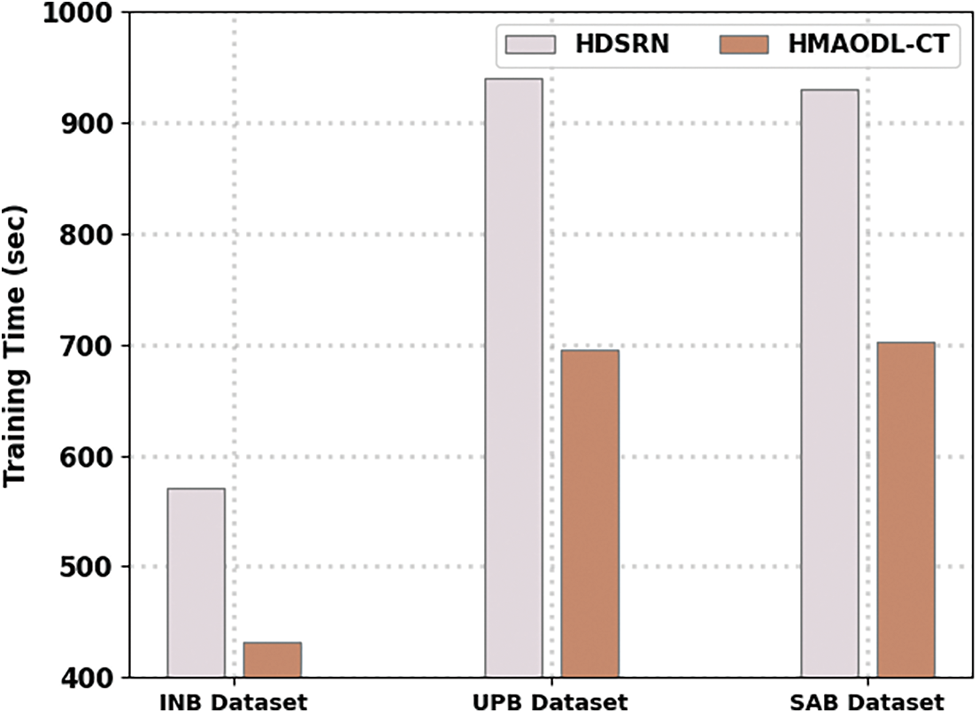
Figure 7: TRT analysis of the HMAODL-CT approach under three databases

Fig. 8 signifies the testing time (TST) analysis of the HMAODL-CT algorithm with the current HDSRN approach. The experimental outcomes show the HMAODL-CT approach provides minimal values of TST under all databases. For example, on the INB database, the HMAODL-CT algorithm has rendered a lower TST of 2 s while the HDSRN technique has reached an increased TST of 3 s. Furthermore, on the UPB database, the HMAODL-CT technique has offered a lower TST of 4 s, while the HDSRN approach has gained an increased TST of 8 s. Also, on the SAB database, the HMAODL-CT approach has presented a lower TST of 5 s, while the HDSRN method has reached an increased TST of 8 s.

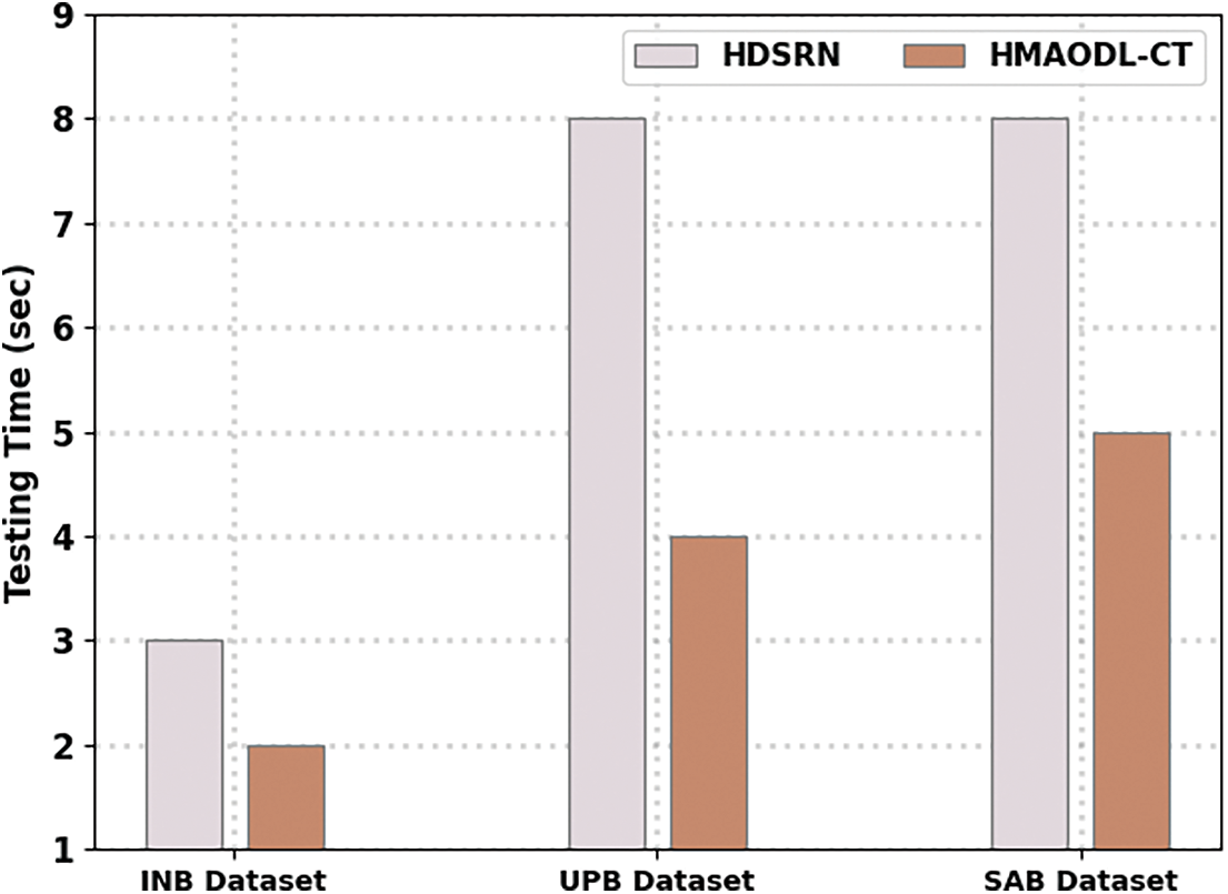
Figure 8: TST analysis of the HMAODL-CT approach under three databases

A detailed comparative analysis is made to affirm the superior outcomes of the HMAODL-CT model [15]. Fig. 9 demonstrates a brief overallaccu assessment of the HMAODL-CT technique with the current approach. The figure revealed that the HMAODL-CT system had attained increasing values of overallaccu. For example, on the INB database, the HMAODL-CT model has depicted a maximum overallaccu of 99.97% while the HDSRN methodology has decreased overallaccu by 99.70%. Next, on the UPB database, the HMAODL-CT approach has shown a maximum overallaccu of 99.97%, while the HDSRN technique has decreased overallaccu by 99.86%. Finally, on the SAB database, the HMAODL-CT algorithm has represented a maximum overallaccu of 99.99% while the HDSRN approach has decreased overallaccu by 99.97%.

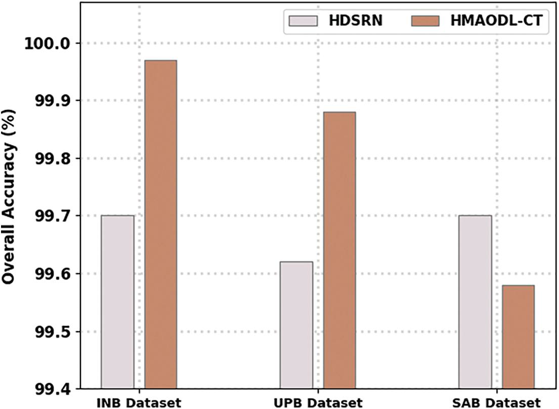
Figure 9: Overall accuracy analysis of the HMAODL-CT approach under three databases

Fig. 10 illustrates a detailed averageaccu assessment of the HMAODL-CT technique with the existing method. The figure specified the HMAODL-CT approach had reached increasing values of averageaccu. For example, on the INB database, the HMAODL-CT technique has portrayed a maximum averageaccu of 99.58%, while the HDSRN algorithm has decreased averageaccu by 99.70%. Next, on the UPB database, the HMAODL-CT model has described a maximum averageaccu of 99.89%, whilethe HDSRN approach has resulted in decreased averageaccu of 99.83%. At last, on the SAB database, the HMAODL-CT model has shown a maximum averageaccu of 99.98%, while the HDSRN model has resulted in decreased averageaccu of 99.97%.

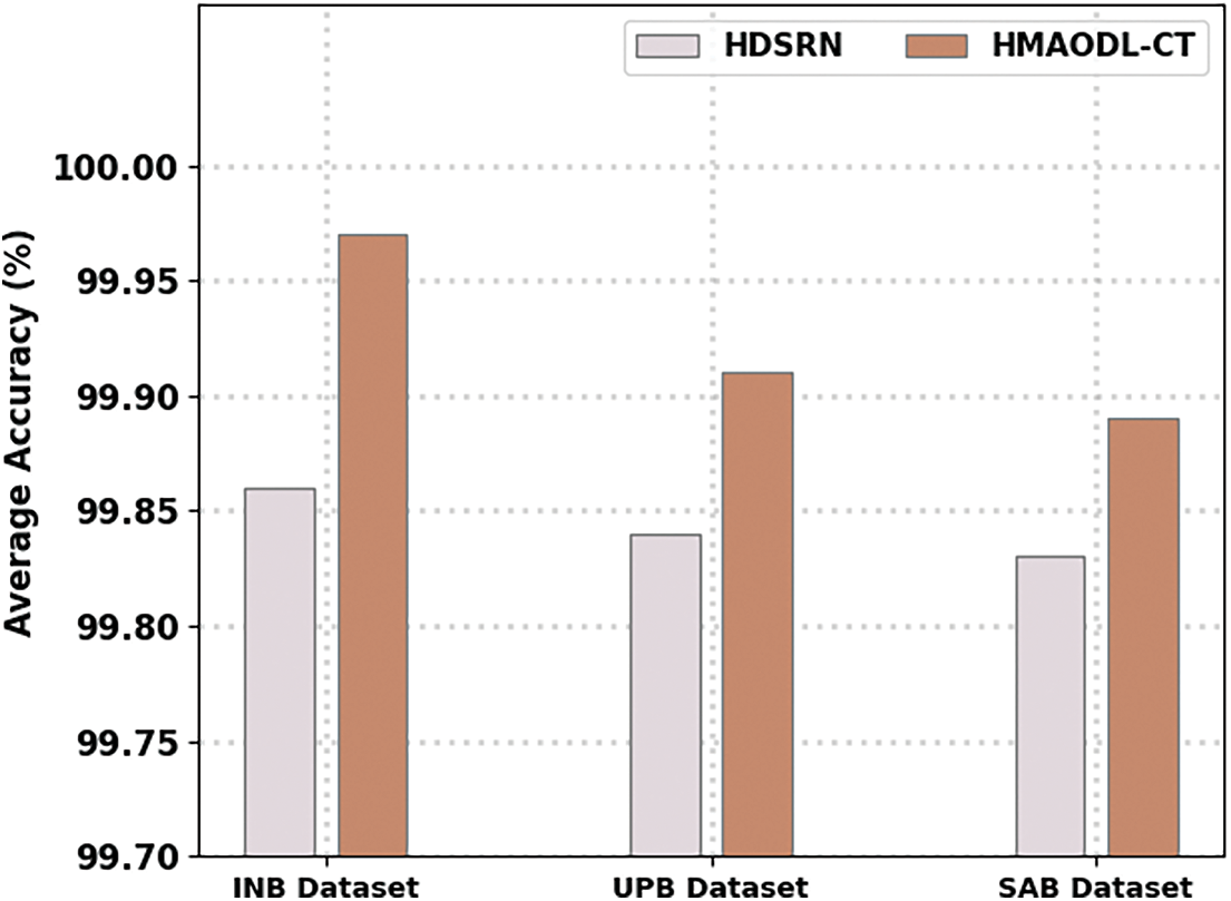
Figure 10: Average accuracy analysis of the HMAODL-CT approach under three databases

Fig. 11 illustrates a brief kappa assessment of the HMAODL-CT technique with the existing approach. The figure designated the HMAODL-CT algorithm has achieved increasing values of kappa. For example, on the INB database, the HMAODL-CT approach has shown a maximum kappa of 99.58%, while the HDSRN technique has decreased kappa by 99.70%. Next, on the UPB database, the HMAODL-CT method has portrayed a maximum kappa of 99.89%, while the HDSRN approach has decreased kappa by 99.83%. Finally, on the SAB database, the HMAODL-CT technique has illustrated a maximum kappa of 99.98%, while the HDSRN method has resulted in decreased kappa of 99.97%. These results pointed out the enhanced performance of the HMAODL-CT approach over other techniques on crop type classification.

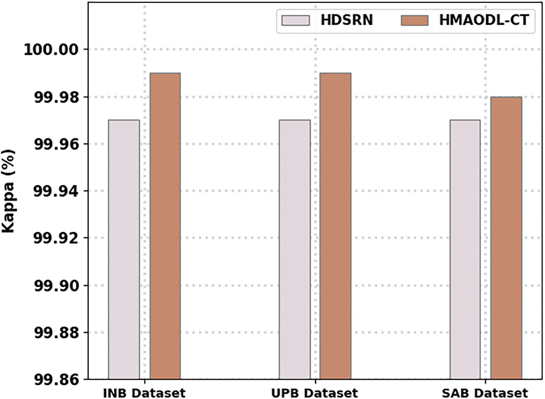
Figure 11: Kappa analysis of HMAODL-CT approach under three databases

5  Conclusion

In this article, a new HMAODL-CTC technique has been developed to classify crops on HSI. The presented HMAODL-CTC technique mainly intends to categorize different types of crops on HSI. Initially, the presented HMAODL-CTC model carries out image preprocessing to improve image quality. Then, the presented HMAODL-CTC model was applied dilated CNN model for feature extraction. For hyperparameter tuning of the dilated CNN model, the HMAO algorithm is utilized. Finally, the presented HMAODL-CTC model uses the ELM model for crop type classification. A comprehensive set of simulations were performed to illustrate the enhanced performance of the presented HMAODL-CTC model. Extensive comparison studies reported the improved performance of the presented HMAODL-CTC model over other compared methods. In future, the proposed model can be tested on large-scale databases.

Acknowledgement: Princess Nourah bint Abdulrahman University Researchers Supporting Project number (PNURSP2023R384), Princess Nourah bint Abdulrahman University, Riyadh, Saudi Arabia.

Funding Statement: This work was supported by Princess Nourah bint Abdulrahman University Researchers Supporting Project number (PNURSP2023R384), Princess Nourah bint Abdulrahman University, Riyadh, Saudi Arabia.

Conflicts of Interest: The authors declare that they have no conflicts of interest to report regarding the present study.

References

1. P. C. Pandey, H. Balzter, P. K. Srivastava, G. P. Petropoulos and B. Bhattacharya, “Future perspectives and challenges in hyperspectral remote sensing,” Hyperspectral Remote Sensing, vol. 35, pp. 429–439, 2020. https://doi.org/10.1016/B978-0-08-102894-0.00021-8 [Google Scholar] [CrossRef]

2. N. Sulaiman, N. N. Che’Ya, M. H. M. Roslim, A. S. Juraimi, N. M. Noor et al., “The application of hyperspectral remote sensing imagery (hrsi) for weed detection analysis in rice fields: A review,” Applied Sciences, vol. 12, no. 5, pp. 2570, 2022. [Google Scholar]

3. S. Pascucci, S. Pignatti, R. Casa, R. Darvishzadeh and W. Huang, “Special issue hyperspectral remote sensing of agriculture and vegetation,” Remote Sensing, vol. 12, no. 21, pp. 3665, 2020. [Google Scholar]

4. Y. Fu, G. Yang, R. Pu, Z. Li, H. Li et al., “An overview of crop nitrogen status assessment using hyperspectral remote sensing: Current status and perspectives,” European Journal of Agronomy, vol. 124, pp. 126241, 2021. [Google Scholar]

5. K. Bhosle and V. Musande, “Evaluation of deep learning CNN model for land use land cover classification and crop identification using hyperspectral remote sensing images,” Journal of the Indian Society of Remote Sensing, vol. 47, no. 11, pp. 1949–1958, 2019. [Google Scholar]

6. P. Sinha, A. Robson, D. Schneider, T. Kilic, H. K. Mugera et al., “The potential of in-situ hyperspectral remote sensing for differentiating 12 banana genotypes grown in Uganda,” ISPRS Journal of Photogrammetry and Remote Sensing, vol. 167, no. 4, pp. 85–103, 2020. [Google Scholar]

7. N. T. Basinger, K. M. Jennings, E. L. Hestir, D. W. Monks, D. L. Jordan et al., “Phenology affects differentiation of crop and weed species using hyperspectral remote sensing,” Weed Technology, vol. 34, no. 6, pp. 897–908, 2020. [Google Scholar]

8. H. Yu, B. Kong, Y. Hou, X. Xu, T. Chen et al., “A critical review on applications of hyperspectral remote sensing in crop monitoring,” Experimental Agriculture, vol. 58, pp. 85–103, 2022. [Google Scholar]

9. L. Lei, X. Wang, Y. Zhong, H. Zhao, X. Hu et al., “DOCC: Deep one-class crop classification via positive and unlabeled learning for multi-modal satellite imagery,” International Journal of Applied Earth Observation and Geoinformation, vol. 105, pp. 102598, 2021. [Google Scholar]

10. L. Agilandeeswari, M. Prabukumar, V. Radhesyam, K. L. B. Phaneendra and A. Farhan, “Crop classification for agricultural applications in hyperspectral remote sensing images,” Applied Sciences, vol. 12, no. 3, pp. 1670, 2022. [Google Scholar]

11. M. A. Hamza, F. Alrowais, J. S. Alzahrani, H. Mahgoub, N. M. Salem et al., “Squirrel search optimization with deep transfer learning-enabled crop classification model on hyperspectral remote sensing imagery,” Applied Sciences, vol. 12, no. 11, pp. 5650, 2022. [Google Scholar]

12. S. Meng, X. Wang, X. Hu, C. Luo and Y. Zhong, “Deep learning-based crop mapping in the cloudy season using one-shot hyperspectral satellite imagery,” Computers and Electronics in Agriculture, vol. 186, pp. 106188, 2021. [Google Scholar]

13. K. Bhosle and B. Ahirwadkar, “Deep learning convolutional neural network (cnn) for cotton, mulberry and sugarcane classification using hyperspectral remote sensing data,” Journal of Integrated Science and Technology, vol. 9, no. 2, pp. 70–74, 2021. [Google Scholar]

14. L. Wei, K. Wang, Q. Lu, Y. Liang, H. Li et al., “Crops fine classification in airborne hyperspectral imagery based on multi-feature fusion and deep learning,” Remote Sensing, vol. 13, no. 15, pp. 2917, 2021. [Google Scholar]

15. J. E. Gutierrez, M. Gamarra, M. T. Torres, N. Madera, J. C. C. Sarmiento et al., “Intelligent sine cosine optimization with deep transfer learning based crops type classification using hyperspectral images,” Canadian Journal of Remote Sensing, pp. 1–12, 2022. https://doi.org/10.1080/07038992.2022.2081538 [Google Scholar] [CrossRef]

16. L. Wei, M. Yu, Y. Liang, Z. Yuan, C. Huang et al., “Precise crop classification using spectral-spatial-location fusion based on conditional random fields for UAV-borne hyperspectral remote sensing imagery,” Remote Sensing, vol. 11, no. 17, pp. 2011, 2019. [Google Scholar]

17. H. Wu, H. Zhou, A. Wang and Y. Iwahori, “Precise crop classification of hyperspectral images using multi-branch feature fusion and dilation-based mlp,” Remote Sensing, vol. 14, no. 11, pp. 2713, 2022. [Google Scholar]

18. V. Nyemeesha and B. M. Ismail, “Implementation of noise and hair removals from dermoscopy images using hybrid Gaussian filter,” Network Modeling Analysis in Health Informatics and Bioinformatics, vol. 10, no. 1, pp. 1–10, 2021. [Google Scholar]

19. N. Khan, A. Ullah, I. U. Haq, V. G. Menon, S. W. Baik et al., “SD-Net: Understanding overcrowded scenes in real-time via an efficient dilated convolutional neural network,” Journal of Real-Time Image Processing, vol. 18, no. 5, pp. 1729–1743, 2021. [Google Scholar]

20. L. Abualigah, D. Yousri, M. A. Elaziz, A. A. Ewees, M. A. Al-Qaness et al., “Aquila optimizer: A novel meta-heuristic optimization algorithm,” Computers & Industrial Engineering, vol. 157, no. 11, pp. 107250, 2021. [Google Scholar]

21. D. Li, S. Li, S. Zhang, J. Sun, L. Wang et al., “Aging state prediction for supercapacitors based on heuristic kalman filter optimization extreme learning machine,” Energy, vol. 250, no. 2, pp. 123773, 2022. [Google Scholar]

22. B. C. Kuo, H. H. Ho, C. H. Li, C. C. Hung and J. S. Taur, “A kernel-based feature selection method for svm with rbf kernel for hyperspectral image classification,” IEEE Journal of Selected Topics in Applied Earth Observations and Remote Sensing, vol. 7, no. 1, pp. 317–326, 2014. [Google Scholar]

23. F. Luo, B. Du, L. Zhang, L. Zhang and D. Tao, “Feature learning using spatial-spectral hypergraph discriminant analysis for hyperspectral image,” IEEE Transactions on Cybernetics, vol. 49, no. 7, pp. 2406–2419, 2019. [Google Scholar] [PubMed]

24. Computational Intelligence Group of the Basque University (UPV/EHU“Hyperspectral Remote Sensing Scenes, Computational Intelligence Group of the Basque University (UPV/EHU),” San Sebastian, Spain, 2020. http://www.ehu.eus/ccwintco/index.php/Hyperspectral_Remote_Sensing_Scenes [Google Scholar]