Orthogonal Probability Approximation for Highly Accurate and Efficient Orbit Uncertainty Propagation

1  Introduction

Uncertainty Quantification (UQ) in the context of Space Situational Awareness (SSA) refers to the process of systematically assessing and managing the uncertainties associated with the prediction and tracking of space objects, such as satellites, space debris, and other resident space objects (RSOs) [1,2]. Conjunction analysis, probability of collision estimation, and uncorrelated track association are some of the major areas in SSA that require accurate UQ of the state of an RSO [3,4]. Utilizing conventional methods for these problems can be challenging when the Probability Density Function (PDF) of interest is non-Gaussian or becomes non-Gaussian due to nonlinear dynamics propagation [5]. This phenomenon can be observed in a Monte Carlo simulation when one million initial states of an Earth-bound satellite are propagated over ten days. The final states become so widely distributed in the orbital space that the resulting distribution is non-Gaussian [6]. The widely used method of propagating the State Transition Matrix (STM) and system states to the final time, and linearly mapping the a priori uncertainty to the final state, has the following flaw: the system dynamics are linearized for STM propagation, and the PDF at the final state is assumed to be Gaussian in nature [4,7]. This issue can be addressed by including higher-order derivatives with State Transition Tensor (STT) methods in the mapping of the final PDF [8,9]. However, such methods require the higher-order partial derivatives of the force models with respect to the state variables to be either computed or approximated [10–12]. This necessitates a trade-off between accuracy and computational cost [13,14]. Differential algebra (DA) techniques have been used for accurate nonlinear uncertainty propagation. By implementing a new algebra of Taylor polynomials, any function of n-dimensional variables can be expanded into its Taylor polynomial of arbitrary order, along with the function evaluation [15]. For a general ODE with given initial conditions, this allows for the computation of an arbitrary order expansion of the solution flow. Based on the DA technique, the uncertainties of a dynamic system can be propagated using a higher-order Taylor expansion of the statistical moments. DA-based uncertainty propagation has been used for asteroid encounter analysis, preliminary orbit determination, propagation of orbit uncertainties, and orbital conjunction analysis [16].

Monte Carlo (MC) simulation is currently the most reliable high-fidelity method for uncertainty propagation. The outcomes of these simulations can be used in conjunction analysis, developing kernel density estimates, or histograms to represent the posterior PDF [17]. The accuracy of MC-based methods is shown to be inversely proportional to the square root of the number of sample points, meaning even a marginal increase in accuracy requires the propagation of a large number of samples. The Brute Force Monte Carlo (BFMC) algorithm, developed by NASA’s Conjunction Assessment Risk Analysis team, is a high-fidelity tool for estimating the collision probability of Earth-orbiting satellites [18]. It targets long-term or repeating encounters between closely spaced, high-value Earth-orbiting satellites. The algorithm uses higher-order theory models from the Astrodynamics Support Workstation, including the latest updates of the atmospheric parameters for the High Accuracy Satellite Drag Model (HASDM). Including parametric uncertainty in the orbital dynamics force model requires at least a 7-dimensional state space to quantify the uncertainty in the dynamics. For a Gaussian PDF in a 7-dimensional space, more than 10,000 Monte Carlo samples are needed to obtain at least one sample to land in the region with probability values below 10−4. Hence, in higher-dimensional spaces, Monte Carlo simulations become very expensive for obtaining the PDF associated with low-probability events that occur beyond 3σ extremal bounds.

Gaussian Mixture Models (GMM) and Polynomial Chaos Expansions (PCE) are more recent methods of UQ in astrodynamics. GMM characterizes the initial uncertainty as a combination of several Gaussian PDFs, each of which is propagated forward in time and then recombined to create the posterior PDF [19,20]. This method assumes that the final PDF can be well represented by the Gaussian mixture, and it is superior to MC methods in terms of computational cost as dimensionality increases [21,22]. In PCE, a functional representation of the system response is used for UQ. Such techniques have been applied to the quantification of uncertainty in astrodynamics [23–25]. The problem of orbit uncertainty propagation in short arcs has been addressed using the method of admissible regions and a new Arbitrary Polynomial Chaos (APC) method [26]. The admissible region method attempts to solve the initial orbit determination problem involving short-arc optical observations, such as angles and angular rates. Combining the stochastic collocation to determine the APC coefficients significantly increases the computational efficiency of the APC method when compared to the MC method. Numerical methods to solve the Fokker-Planck equation can also capture the evolution of the PDF in nonlinear dynamical systems. Some of these methods include Unscented Transformation (UT) and tensor decomposition in combination with Chebyshev spectral differentiation [27,28].

In recent works, an algorithm for orbital conjunction probability analysis of non-Gaussian distributions with model uncertainties and long encounter times, dubbed CRATER, has been introduced [29]. For collisions involving highly non-Gaussian PDFs, the algorithm approximates the PDF as a GMM, and the collision probability is evaluated using Coppola’s method, excluding mixtures that are beyond 6σ from each other. By using a nonlinearity index to determine the number of mixtures needed in a GMM, the algorithm is made adaptive to deal with several collision types. Though the algorithm is comparable to GMMs in terms of accuracy, it has been shown to be computationally more efficient. A new approach involving the Petri Net model has been used to investigate the impact of the space debris flux on the estimation of collision probabilities between space debris and Low Earth Orbit (LEO) satellites [30]. Using weighted and bipartite graphs that consist of two kinds of nodes (places and transitions), Petri nets can be used to model and simulate the behavior of space debris systems. Utilizing the space debris flux distribution of a specific year, the simulation is applied to a group of well-known LEO satellites with different orbital parameters to estimate the collision probabilities within the next 12 years. Results obtained from this model show that satellites in LEO between altitudes of 600 km and 1000 km with inclination angles between 90° and 100° are expected to experience frequent collisions by 2030. A more recently published work propagates orbit uncertainty using an orbit deviation propagation approach. It combines an analytical two-body deviation propagation solution with a Deep Neural Network (DNN) output to compensate for the errors between the two-body and high-fidelity dynamic solutions. This fast approach propagates the mean and covariance by combining the Unscented Transformation process with DNN-based deviation propagation [31]. Another approximation algorithm, called Global-Local Orthogonal MAPping (GLOMAP), uses the properties of dynamical systems to approximate the PDF and its evolution along the trajectories of an n-dimensional state space. It is a multi-resolution approximation algorithm that is robust, as it can accurately characterize the noise and uncertainty in the data [32]. The algorithm is applied to compute the evolution of the PDF of a polar sun-synchronous orbit with J2 perturbation. Results indicate that for a propagation time of 2 h, the GLOMAP algorithm yields a maximum PDF approximation error of 12%, which the authors consider to be reasonable [33]. At higher levels of uncertainty, all the above-mentioned methods do not provide a general description of the posterior PDF without extreme computational cost.

In this paper, a conceptual explanation of the Orthogonal Probability Approximation (OPA) is introduced in Section 2. A one-dimensional illustration of the concept is provided in Section 2.1. This is followed by the development of PDF modulation for non-conservative systems and illustrations of grid filtering techniques in Sections 2.2 and 2.3, respectively. A general overview of implementing OPA is given in Section 2.4. Linear system validation consists of using OPA to obtain the posterior PDF of a simple harmonic oscillator with 2-dimensional (2D) state uncertainty in position and velocity, as presented in Section 2.5. Section 3 introduces the numerical results of using OPA for UQ in nonlinear systems. First, OPA is used to quantify the posterior PDF of a conservative, and a non-conservative Duffing oscillator in Sections 3.1 and 3.2, respectively. Both 2-dimensional (2D) and 3-dimensional (3D) uncertainties are investigated, involving state and parametric uncertainties. Numerical outcomes are compared with the computation time and accuracy of classical Monte Carlo simulations. Then, OPA is applied to quantify the uncertainty in the state of a satellite whose motion is confined to a plane, as shown in Section 3.3. Finally, a discussion of the results is given in Section 4, and concluding remarks are presented in Section 5.

2  OPA Methodology

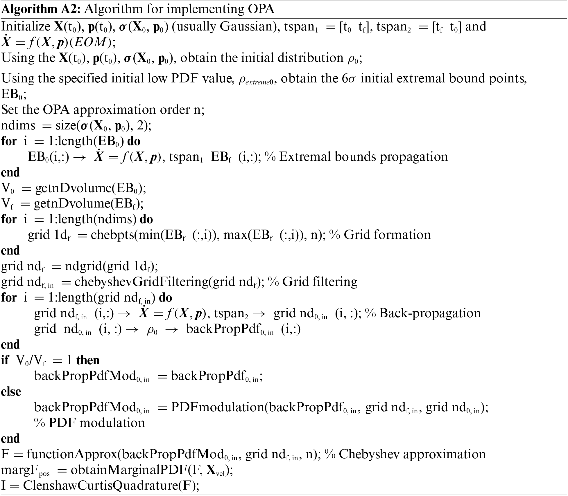
The method of OPA was originally introduced in previous works [6,34,35]. Being a highly efficient method for lower-dimensional analysis, it provides a very precise description of the posterior PDF at orders of magnitude lower computational cost than the classical Monte Carlo approach. This method also provides a more accurate definition of the low probability density region of the PDF than the Monte Carlo approach. The objective of OPA is to quantify uncertainty or determine the probability distribution of a dynamic system at a future time of interest, tf, provided the probability distribution of the system is known at the initial time, t0. An overview of the OPA method is presented as a flowchart in Fig. 1. For a general n-dimensional dynamical system, the initial states, parameters, and their initial uncertainties are specified at the beginning of the simulation. Next, the OPA parameters, such as the number of extremal bound points and the approximation order, are determined. This is followed by the propagation of the extremal bound points from t0 to tf using the equations of motion. An n-dimensional Chebyshev grid is then created using the extremal bounds, and grid filtering is applied. The filtered grid points are subsequently backpropagated to t0, and the known initial PDF values at the backpropagated grid points are referenced to tf. Depending on whether the system dynamics are conservative or non-conservative, the referenced PDF values are modulated using the procedure described in Section 2.2. The orthogonal Chebyshev polynomials are then used to approximate the n-dimensional PDF, after which the marginal PDF values are obtained by integrating the approximated PDF with respect to the system’s random variables. The final step is the computation of the cumulative probability integral. The sections below provide a detailed description of the OPA methodology.

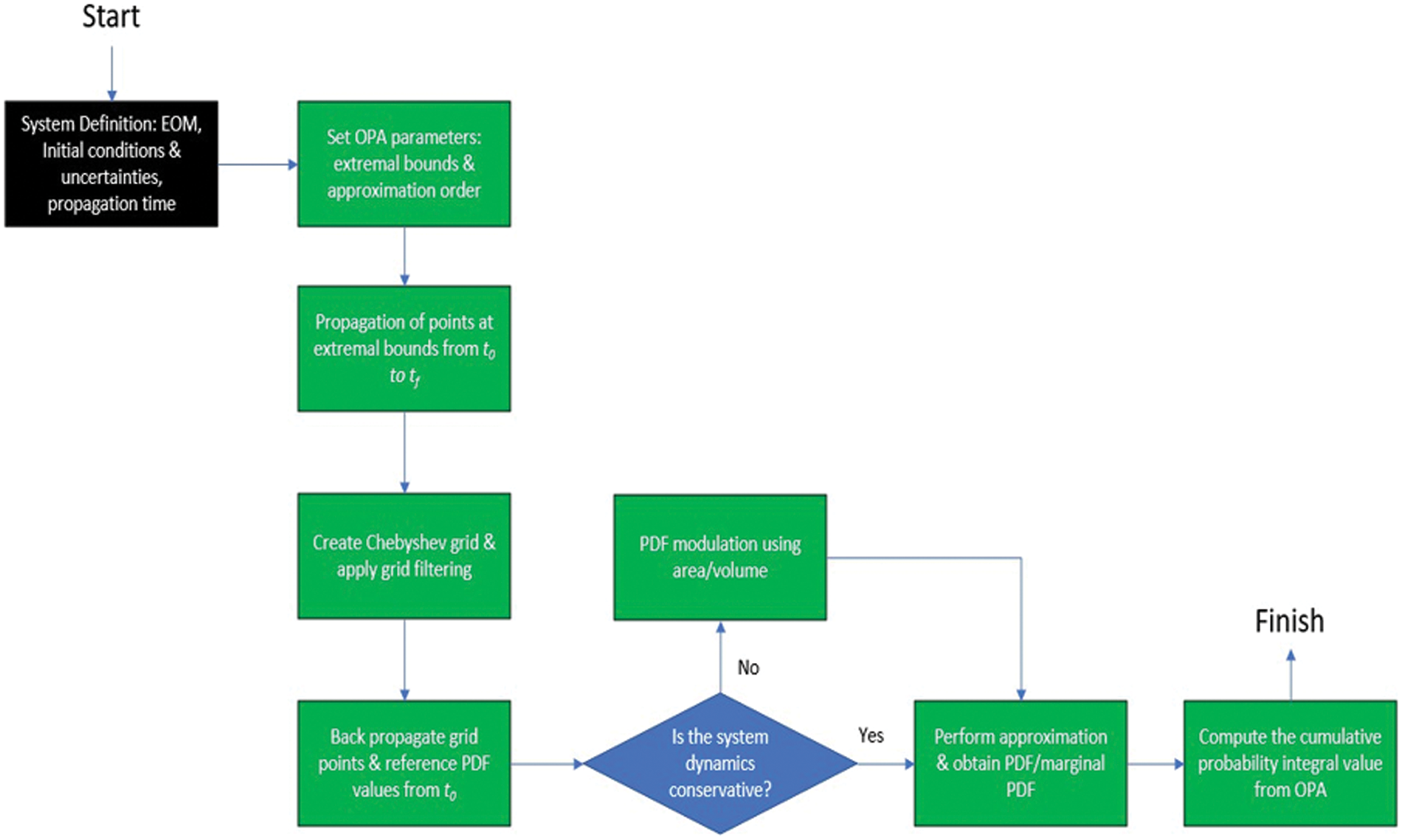
Figure 1: OPA overview flowchart (EOM: Equations of Motion)

2.1 Basics

This problem of uncertainty quantification in one dimension is depicted in Fig. 2a, where the solid blue curve denotes the known distribution at t0, and the broken green line indicates the unknown distribution at tf. In the first step, confinement of the region of interest at tf is done. This is the region in which the approximation of the unknown final PDF will be performed. This is done by locating the state space points at t0 whose PDF values match the boundary PDF value of interest. In this work, a PDF value equivalent to 6σ in a Gaussian distribution is specified as the boundary PDF value at t0. These state space points are then propagated to tf using the ordinary differential equations (ODEs) that govern the system. In this work, unless specified otherwise, all the ODEs are numerically integrated using MATLAB’s Runge-Kutta 45 integrator (ode45) with the tolerance values, both relative and absolute, set to 10−8. The region between these state space points, or their generalized surface in higher dimensions, is referred to as the region of extremal probability. This is depicted in Fig. 2b, where the red dashes on the x-axis mark the extremal bounds. Obtaining the extremal bounds at t0 is straightforward for well-characterized distributions (e.g., Gaussian or Cauchy). For more complex a priori distributions, a randomized searching method would be required. Unless stated otherwise, the initial distribution for all the cases presented in this work is Gaussian.

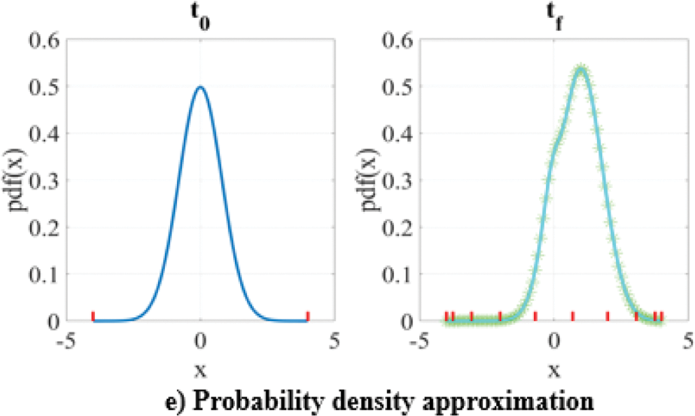
Figure 2: OPA scheme illustrated using a 1D PDF example

After locating the extremal bounds at tf, the space between them is populated with grid points whose PDF values will be computed from the a priori distribution and then used in the subsequent approximation process. Fig. 2c depicts cosine nodes distributed between the extremal bounds at tf. To achieve this, each evaluation node at tf is backpropagated to t0 using the system ODEs, with the state information of these nodes at tf serving as the initial condition. The PDF value at the backpropagated grid points is obtained by comparing the a priori distribution with the backpropagated state value of these nodes. According to Liouville’s theorem, these PDF values always remain unchanged for conservative systems. Hence, these PDF values are referenced to the grid points at tf, where they are utilized to generate a functional approximation of the final probability distribution using Chebyshev polynomials, f(x)≅∑k=0nakφk(x), where, n is the order of approximation, φk(x) is the Chebyshev polynomial of order k in x, and ak is the approximation coefficient. Fig. 2d depicts the back-propagation of each of the grid points, and Fig. 2e shows the resulting approximation for the posterior PDF. It is important to note that the mapping of the known PDF values at the backpropagated grid points occurs from t0 to tf through the utilization of Liouville’s theorem. This step is also known as referencing the PDF values. The order of the approximation, n, is determined by the accuracy requirements of the PDF approximation, and the corresponding coefficients are estimated using a least-squares process. Since the Chebyshev polynomials φk(x) are orthogonal within the domain of approximation, the matrix inversion step in the least squares process can be executed more efficiently. The approximation process is performed using Chebfun, an open-source MATLAB toolbox for Chebyshev polynomial approximation [36]. Unless specified otherwise, all numerical results shown in this paper were obtained using the Chebfun toolbox.

2.2 PDF Modulation for n-D Non-Conservative Systems

The OPA technique outlined in Section 2.1 is based on Liouville’s theorem which states that the probability density value of a state space point, defined by an a priori distribution with initial conditions, remains constant as long as the point traverses a unique state space trajectory. This is encapsulated in Liouville’s equation [37] as,

dρdt=∂ρ∂t+∑i=1m(∂ρ∂qiqi˙+∂ρ∂pipi˙)=0(1)

where, q, p denote the state variables, and the number of random variables is indicated by m.

This is true only for conservative dynamical systems. For systems that involve non-conservative dynamics, energy may either be removed (e.g., friction and drag) or added (e.g., thruster, solar radiation input on satellite solar panels) to the system. Hence, Eq. (1) is no longer applicable, and the probability density of a given state space point changes with time. This variation can be quantified by the fact that, at any time instant, the integral of the probability density surface with respect to all the random variables must equal one. For example, in the case of dissipative systems, for the integral of the probability density surface to equal one at any instant, the PDF value of a state space point must increase as it moves forward in time. This increase continues until the system reaches a steady state, which has the maximum probability. Conversely, the opposite occurs in a system to which energy is added: the PDF value of a state space point decreases as it moves forward in time.

Fig. 3 illustrates the effect of energy dissipation in a damped Duffing oscillator which is a system with 2 random variables (i.e., position and velocity). As shown, the area covered by the extremal bounds at tf (green) is smaller than the area covered by the extremal bounds at t0 (red). This means that the associated PDF at tf increases in value in proportion to the area shrinkage of the extremal bounds at tf. In Fig. 2d, each back-propagated evaluation node picks up a PDF value based on its location in the state space and the a priori PDF. This PDF value is scaled or modified to reflect the area shrinkage. For problems with two random variables, a local scale factor is adopted for each evaluation node. The area of the triangle for which each evaluation node is a vertex is computed. The area change of each such triangle during back-propagation is tracked and used to compute the scale factor, which is then used to scale the PDF value. If Afi and A0i denote the area of the triangle associated with the i-th evaluation node at tf and t0, respectively, then the associated scale factor, SFi is obtained by,

A0i=12|x100x2001x110x2101x120x2201|i(2)

Afi=12|x10fx20f1x11fx21f1x12fx22f1|i(3)

A0i=12|a001a101a201|i(4)

Afi=12|a0f1a1f1a2f1|i(5)

SFi=A0iAfi(6)

where, a00 (x100, x200), a10 (x110, x210), a20 (x120, x220) represent the vector locations of the triangle vertices/nodes at t0, and a0f (x10f, x20f), a1f (x11f, x21f), a2f (x12f, x22f) represent the vector locations of the triangle vertices/nodes at tf. This PDF modulation process for a single triangle is illustrated in Fig. 4. A systematic repetition of this process is done by constructing adjacent triangles to obtain the scale factors associated with all nodes (i.e., i = 0, 1, 2, ..., n). The referenced PDF value from t0, at each evaluation node is then multiplied/scaled by the scale factor SFi before the Chebyshev approximation step.

Figure 3: 2D Duffing oscillator with damping: shrinking of the extremal bounds when the system propagates through state space. Area formed by the extremal bounds at tf (green) is smaller than the area formed by the extremal bounds at t0 (red)

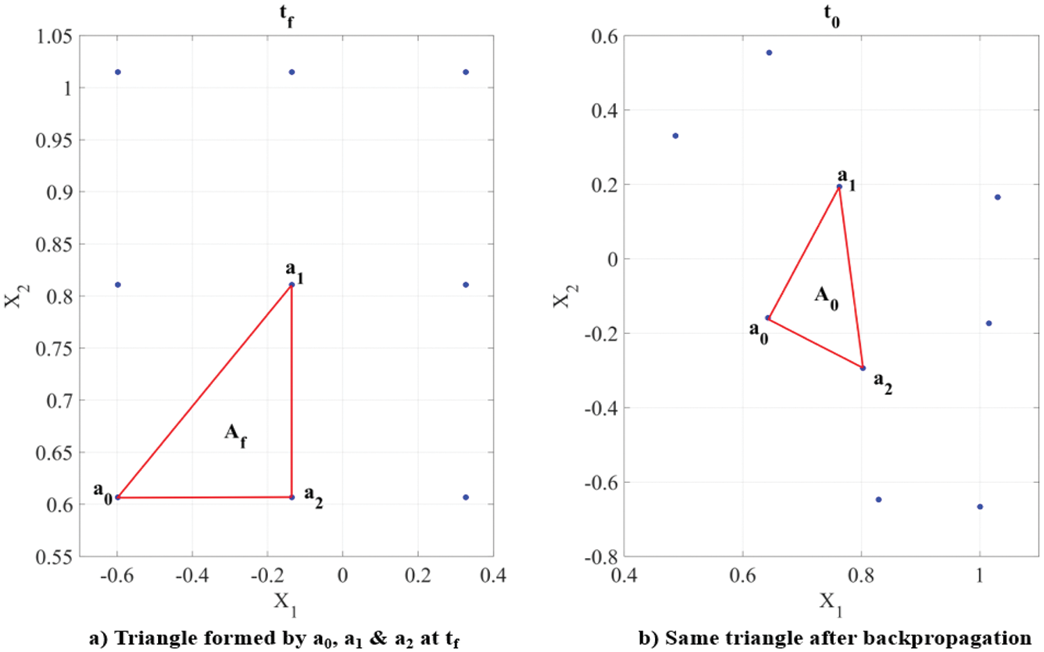
Figure 4: Sample PDF modulation using triangles in a 2D problem

Similarly, for a non-conservative dynamical system with 3 random variables (x1, x2 and x3), a local scale factor is adopted for each evaluation node. The volume of the tetrahedron for which each evaluation node is a vertex is computed. The volume change of each such tetrahedron during back-propagation is tracked and used to compute the scale factor, which is then applied to scale the PDF value. If Vfi and V0i denote the volume of the tetrahedron associated with the i-th evaluation node at tf and t0, respectively, and if SFi is the associated scale factor, then,

V0i=13!|x110−x100x120−x100x130−x100x210−x200x220−x200x230−x200x310−x300x320−x300x330−x300|i(7)

Vfi=13!|x11f−x10fx12f−x10fx13f−x10fx21f−x20fx22f−x20fx23f−x20fx31f−x30fx32f−x30fx33f−x30f|i(8)

V0i=13!|a10−a00a20−a00a30−a00|i(9)

Vfi=13!|a1f−a0fa2f−a0fa3f−a0f|i(10)

SFi=V0iVfi(11)

where a00, a10, a20, a30 represent the vector locations of the tetrahedron vertices at t0 and a0f, a1f, a2f, a3f represent the vector locations of the tetrahedron vertices at tf. This process is illustrated for a single tetrahedron in Fig. 5. The process is systematically repeated to obtain the scale factors associated with each evaluation node, after which they are used to scale the referenced PDF values at each node before they are passed to the approximation step. For a non-conservative dynamical system with n random variables, the scale factor associated with each evaluation node is obtained by evaluating the hypervolume change associated with the corresponding n-dimensional simplex. Using linear algebra, the scale factor associated with the i-th evaluation node can be computed by tracking the hypervolume change of the corresponding n-dimensional simplex,

V0i=1n!|x110−x100x120−x100…x1n0−x100x210−x200x220−x200…x2n0−x200⋮⋮⋮⋮xn10−xn00xn20−xn00…xnn0−xn00|i(12)

Vfi=1n!|x11f−x10fx12f−x10f…x1nf−x10fx21f−x20fx22f−x20f…x2nf−x20f⋮⋮⋮⋮xn1f−xn0fxn2f−xn0f…xnnf−xn0f|i(13)

V0i=1n!|a10−a00a20−a00…an0−a00|i(14)

Vfi=1n!|a1f−a0fa2f−a0f…anf−a0f|i(15)

SFi=V0iVfi(16)

where, a00, a10, ..., an0 represent the vector locations of the simplex vertices at t0, and a0f, a1f, ..., anf represent the vector locations of the simplex vertices at tf. Despite being a very precise way to scale the n-dimensional PDF, this local technique is computationally intensive. An alternative, albeit less accurate, approach is to estimate the scale factor by computing the overall hypervolume shrinkage associated with the n-dimensional extremal bounds. This can be done using the convexhull function in MATLAB.

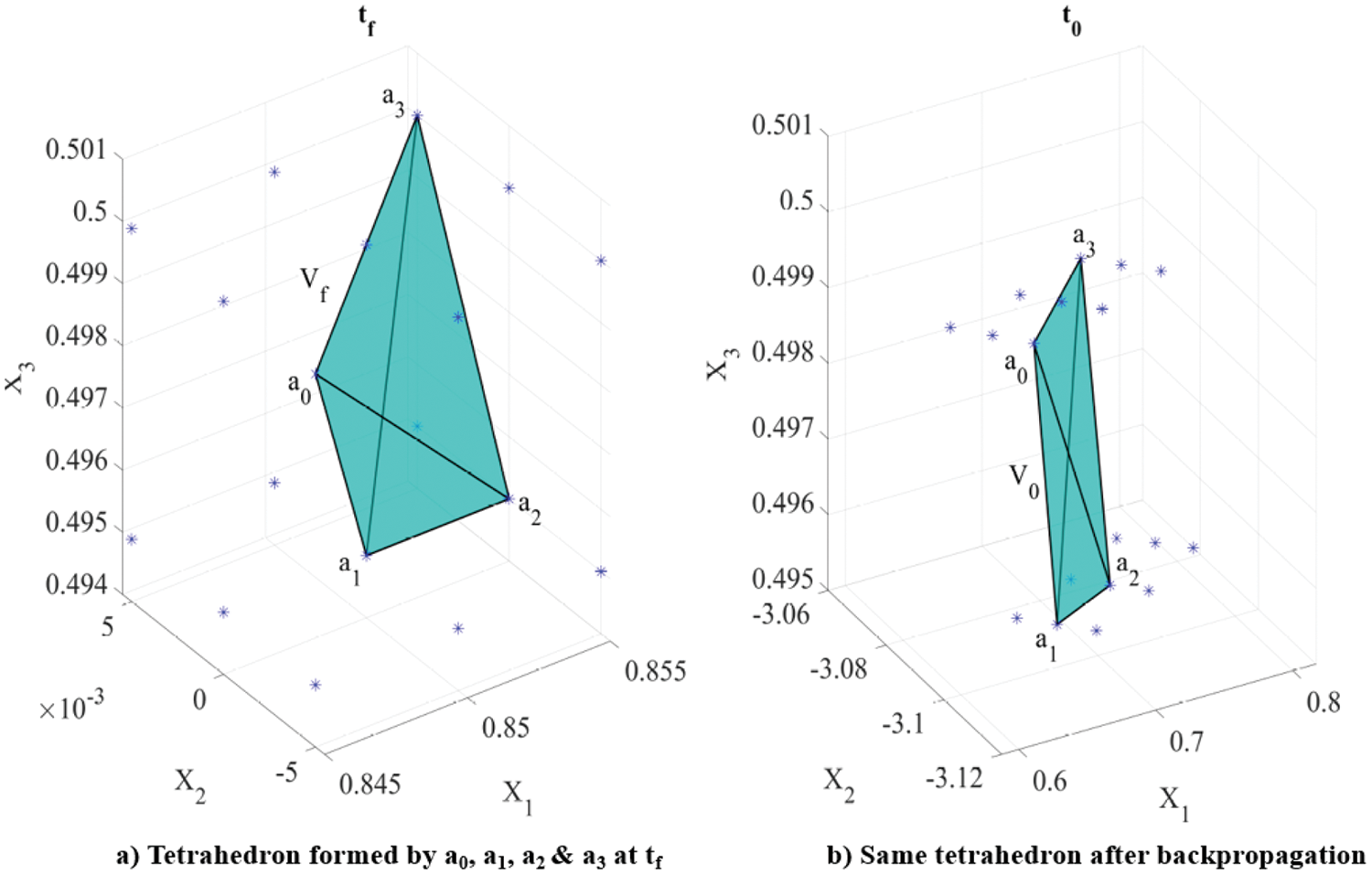
Figure 5: Sample PDF modulation using tetrahedrons in a 3D problem

2.3 Chebyshev Grid Filtering

An important step in OPA is the back-propagation of the grid points (Fig. 2d). This step presents two key challenges that need to be addressed: i) the curse of dimensionality, and ii) the system’s nonlinear dynamics. In lower-dimensional problems, up to 2D, even with an approximation order as high as 70, the time required for the back-propagation of, for example, 4900 (= 70 × 70) points is significantly less than the time required for a Monte Carlo simulation that achieves the same PDF approximation accuracy. However, in higher dimensional PDF approximation, the number of points created in a tensorial grid increases exponentially. But most of these grid points are clustered near the boundary where the PDF value is essentially zero. Hence, with each dimension, the number of grid points required for PDF approximation increases by nearly an order of magnitude, of which only a small fraction of them are in locations where the PDF values are non-zero. This phenomenon is known as the curse of dimensionality [38].

The second challenge is the divergence that can occur during the back-propagation of nonlinear dynamics (i.e., one or more state space variables become extremely large or approach infinity). In Fig. 6, every point on the extremal bounds at tf is obtained by forward propagation of the points on the extremal bounds at t0. Each point in the overlaid Chebyshev grid is a state space point that, in principle, can be backpropagated to t0. In theory, after back-propagation, every grid point that lies within the extremal bounds at tf (i.e., an internal grid point) will land within the extremal bounds at t0, and every grid point that lies outside the extremal bounds at tf (i.e., an external grid point) will land outside the extremal bounds at t0. However, in practice, for nonlinear systems, some of these external grid points may land far outside the extremal bounds at t0, and some may even diverge to infinity. Additionally, it is unnecessary to backpropagate these points, as the PDF value at these points is negligible (nearly zero) and not of interest to the problem. To address these issues, points outside the extremal bounds are filtered out, and only the points within the extremal bounds are backpropagated. This filtering improves the efficiency of OPA.

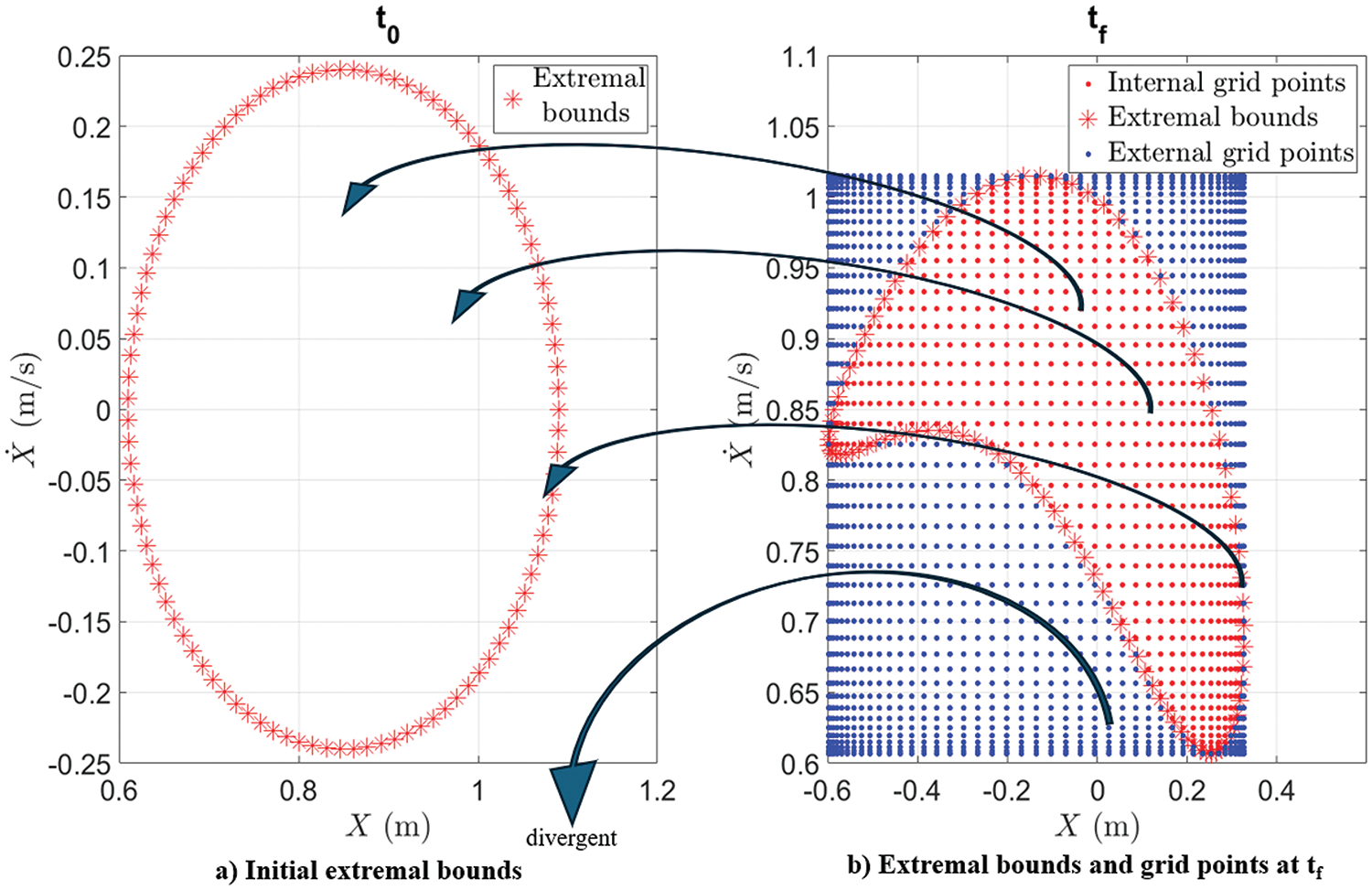
Figure 6: Divergence during back-propagation in nonlinear systems

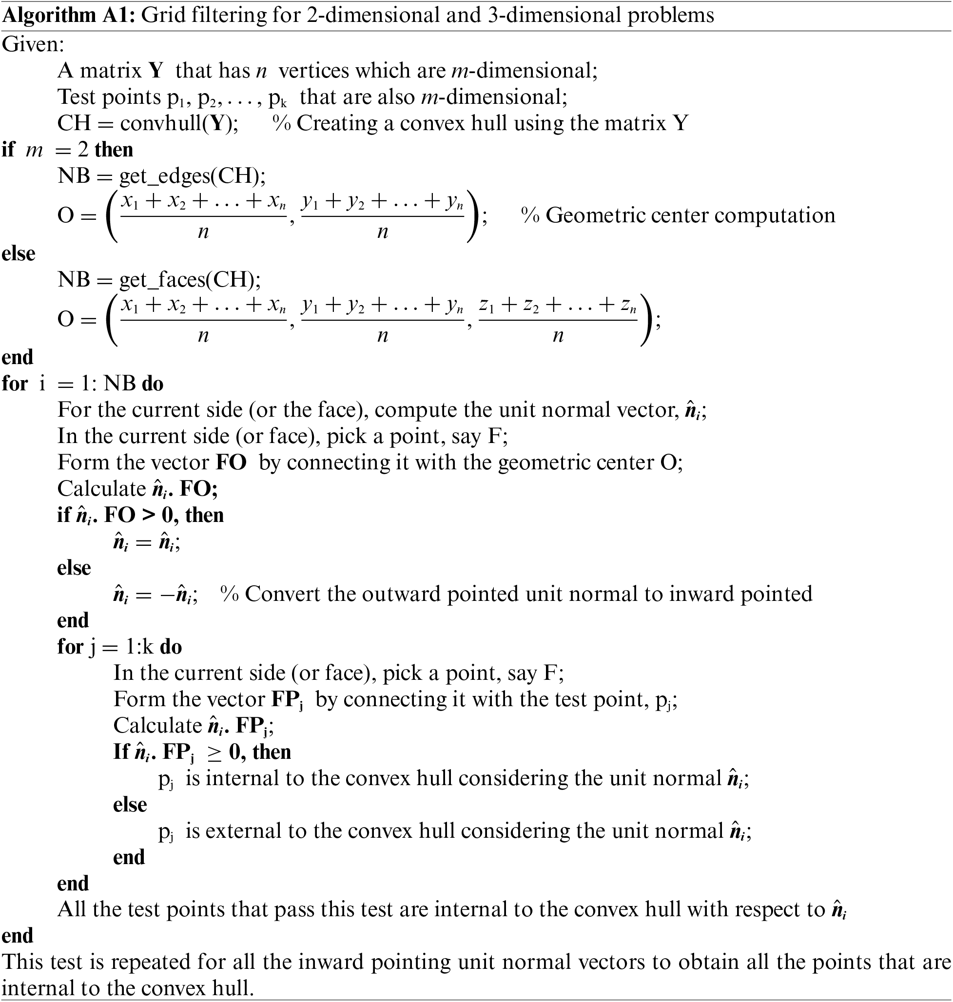
The grid filtering implemented in this paper uses dot products to determine which grid points lie within the extremal bounds. For the 2D case, in the rectangle ABCD shown in Fig. 7a, the points p1 and p2 are checked by first computing the unit normal vectors n^1, . . ., n^4 for the four sides of the rectangle ABCD. The next step is to ensure that all the obtained unit normal vectors are pointing inward. This is done by ensuring that the dot product between the normal vector and the vector from the geometric center to a point on the side is positive. Finally, the test point pi is checked to see if it lies within the rectangle by evaluating the dot product between each of the normal vectors and the vector connecting pi to any point on the side. This dot product value must be non-negative for pi to lie inside ABCD.

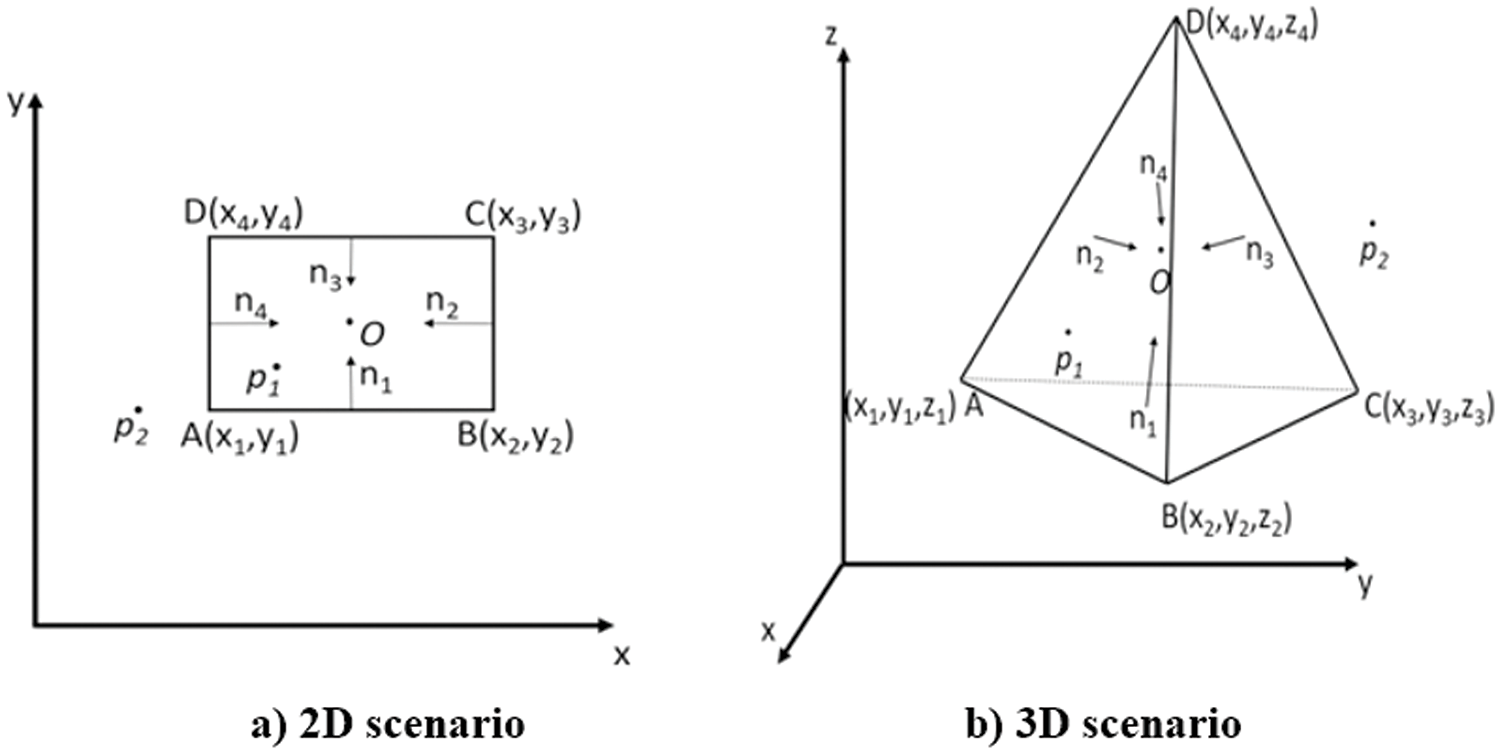
Figure 7: Example of 2D and 3D grid filtering used in OPA

Similarly, for the 3D case, in the tetrahedron ABCD shown in Fig. 7b, the points p1 and p2 are checked by first computing the unit normal vectors for all faces of the tetrahedron. After ensuring the inward pointedness of the unit normal vectors of each face, the dot product between each normal vector and the vector connecting the test point pi to any point on the face is computed. If this dot product is non-negative, then pi lies inside the tetrahedron ABCD. The detailed steps of the process are shown in Algorithm A1 in Appendix A. Algorithm A1 can be applied to any n-sided polygon or n-faced polyhedron. For dimensions higher than 3D, the same dot product inequality check is applied for grid filtering. However, this requires the computation of the null space to obtain the unit normal vectors for each simplex of the n-D convex hull. These procedures are documented and implemented in a user-created MATLAB function, inhull [39].

2.4 Implementation and Validation of OPA

All the steps of OPA described so far are encapsulated in the flowchart shown in Fig. 1. When implementing OPA for nonlinear systems, Monte Carlo (MC) simulations are used to validate the outcomes of OPA. The first step is to create a significant number of sample/test points (i.e., initial conditions) based on the system’s initial known distribution. Typically, around 1 million samples are generated to achieve a reasonable approximation of 6σ extremal bounds. Each of these sample points is then propagated to tf, after which the kernel density estimator is used to generate the PDF from these propagated sample points. As in the OPA simulation, marginal PDFs and the cumulative probability integral are computed. The accuracy of the cumulative probability integrals from the OPA simulation and MC simulation are then compared. Because the initial PDF is truncated in these simulations, according to probability theory, the cumulative probability integral should remain constant between the initial and final PDFs and should be very close to one if the initial PDF is truncated at a 6σ distance from the mean. The approximation order and the number of samples are chosen such that both OPA and MC simulations achieve the same level of accuracy. Consequently, computational efficiency is quantified, for the same level of accuracy of the cumulative integral, by recording the runtime for each method. Algorithm A2 describes the sequence of steps required to implement OPA for a general n-dimensional dynamical system. All the numerical experiments shown in this paper were run on an HDD desktop computer with an Intel(R) Core(TM) i7 processor at a clock speed of 3.4 GHz and 16 GB RAM.

2.5 Validation of OPA via Linear Covariance Propagation

A simple undamped linear system with a unit mass is chosen as a representative of linear systems to validate the implementation of OPA,

X˙=[01−ωn20]X,X˙=AX(17)

where, X=[xx˙]T and ωn is the natural frequency. The relevant OPA simulation parameters can be found in Table 1. In this dynamic system with two random variables, position, and velocity, the 6σ initial extremal bounds of the Gaussian distribution are defined using 100 points. The initial covariance for this dynamic system is given by P0 = diag([0.032 0.052]). Here, Liouville’s theorem is used to place 100 points at the 6σ bounds from the mean values of position and velocity shown in Table 1. First, the eigenvalues and eigenvectors of the initial covariance matrix are obtained. Then, a set of random points on the surface of an n-dimensional unit sphere is generated. The dimension of this set of points corresponds to the dimensionality of the problem, and the cardinality of this set is the number of extremal bound points specified by the user. These random points are then scaled by the product of the initial standard deviation and the value of the extremal bounds (i.e., 6σ for the cases considered in this paper). Finally, these points are oriented using the eigenvectors and translated to lie on the 6σ surface of the distribution, whose mean is specified in Table 1. Nominal values for initial position and velocity, along with the 6σ initial extremal bounds, are propagated through the linear dynamics, Eq. (17), to a chosen final time, tf (Fig. 8).

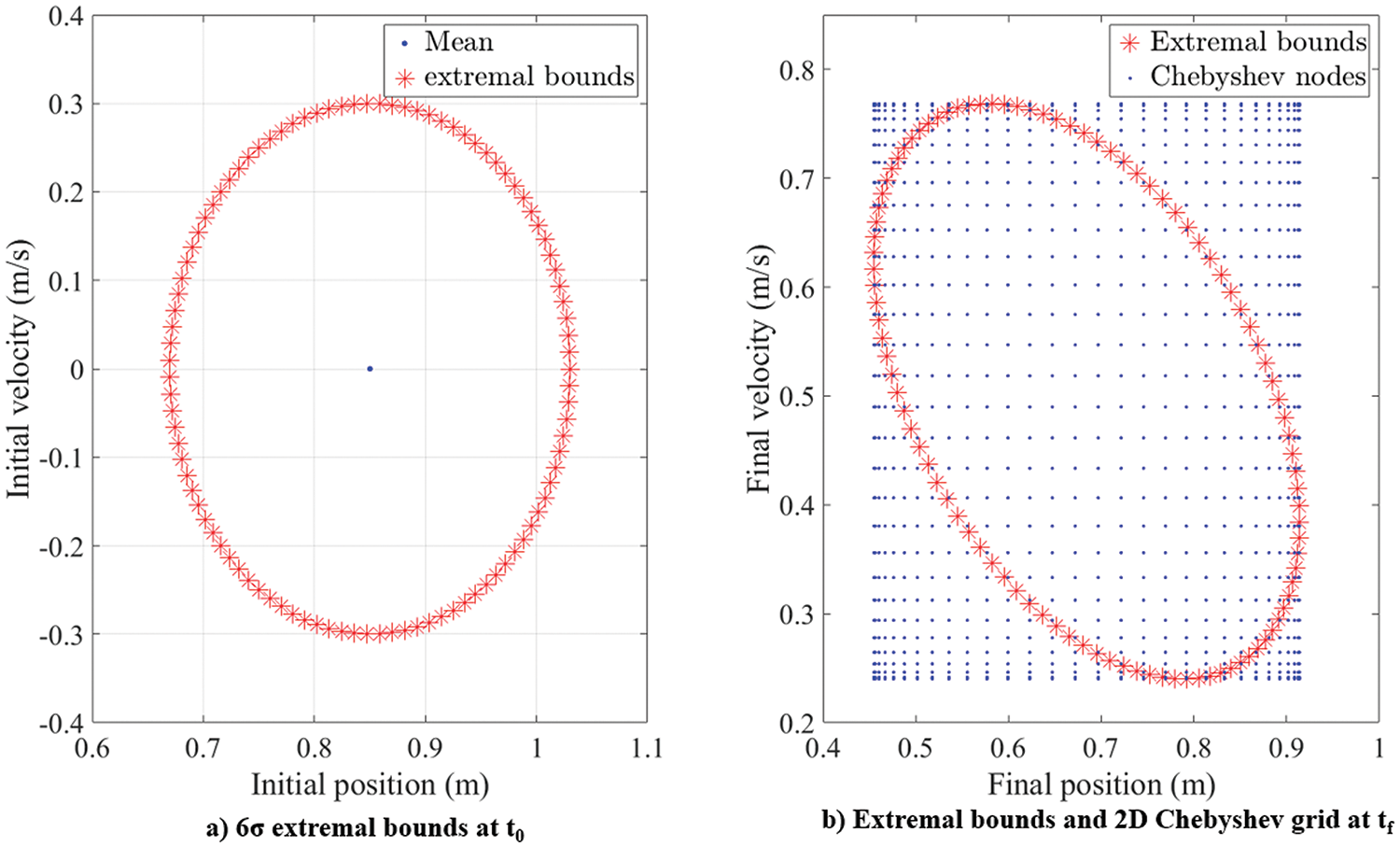
Figure 8: Linear oscillator: initial and final bounds

For an approximation order of 30, the total number of grid points comes to 302 = 900. The probability distribution at any given time is a function of the state variables: position and velocity, which are also the random variables in the linear system. A 2D Chebyshev grid is formed using,

Xij={cos⁡(iπn1),cos⁡(jπn2)},0≤i≤n1,0≤j≤n2,i,j∈Z(18)

For this case, the approximation order for both random variables is set to be equal, i.e., n1 = n2 = n. The grid created encompasses the extremal bounds at tf as shown in Fig. 8. Following the procedure outlined in Section 2.3, the external grid points are eliminated. Each grid point within the extremal bound is back-propagated to the initial time, t0 to obtain the corresponding PDF value (Fig. 9), which, according to Liouville’s theorem, remains unchanged for a conservative system. This set of referenced PDF values at the Chebyshev grid points is then used to approximate the PDF at tf, Fig. 10. The process of approximation is carried out using Chebfun, an open-source MATLAB package that implements Chebyshev polynomial approximations. In a linear dynamic system, the covariance matrix can be numerically propagated to t f using the equation from linear error theory [40],

P˙=AP+PAT(19)

P(t0)=P0(20)

where, A is the system matrix, P is the covariance matrix and P0 is the initial covariance matrix. Using the expression for the PDF value of a multivariate Gaussian distribution,

fanalytical=(2π)−k/2|Σ|−1/2exp⁡(−12(X−µ)TΣ−1(X−µ))(21)

and plugging in μ=[μxfμx˙f] (the propagated mean position and velocity), k = 2 (the cardinality of random variables), and Σ = P (the propagated covariance matrix), the analytical probability density values at the Chebyshev grid points at tf are obtained. Fig. 10 shows the final PDF obtained after approximation, which is compared with the PDF obtained from linear error propagation using Eqs. (19) and (20). The results show errors in the order of 10−7 (Fig. 11). Besides direct comparison of the PDFs, an important accuracy metric in PDF approximations is the evaluation of the total probability integral value, at tf, which is given by,

(If)OPA=∫x∫x˙f(x,x˙)dx˙dx(22)

where, f(x, x˙) is the functional approximation of the PDF. The integral of f(x, x˙) within the 6σ extremal bounds at tf, evaluated using the Clenshaw-Curis quadrature, turns out to be 0.999999991460116 [41]. Since this linear system is assumed to have a Gaussian PDF at t0 that is truncated to the 6σ extremal bounds, the total probability integral at t0 can be computed by converting the distribution to polar coordinates and performing the integration as,

(I0)analytical=12π∫06(∫02πexp(−r22)dθ)rdr(23)

=∫06exp(−r22)rdr

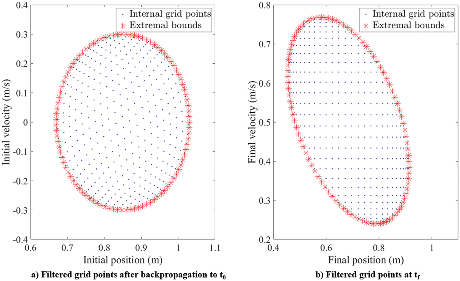
Figure 9: Linear oscillator: filtered grid points before and after back-propagation

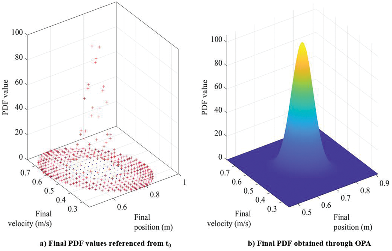
Figure 10: Linear oscillator: performing PDF approximation

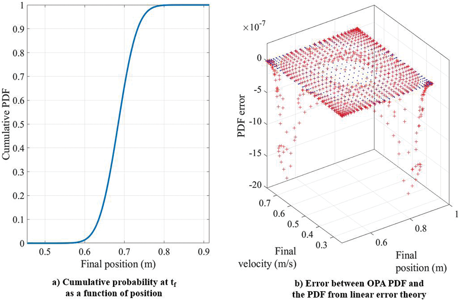
Figure 11: Linear oscillator: cumulative probability and validation using linear error theory

Using integration by substitution with t=r2, it can be shown that,

I0=1−exp(−622)(24)

=0.999999984770020

(I0)analytical=0.999999984770020(25)

According to the fundamental theorem of probability, this value for the total probability integral should always remain constant. Without loss of accuracy, the analytic total probability integral value can be considered the true total probability integral value. It is seen that (If)OPA − (If)analytical is in the order of 10−9, which further demonstrates the accuracy of OPA.

3  Numerical Results

In this section, OPA is used to approximate the PDF of two nonlinear dynamical systems: the Duffing oscillator (undamped and damped), and a satellite in a planar orbit. A Duffing oscillator is a nonlinear oscillator with its overall dynamics described by the equation,

x¨+δx˙+αx+βx3=γcos⁡ωt(26)

where, γ and ω are the amplitude and the angular frequency of the periodic driving force, β is the nonlinear stiffness coefficient, α is the linear stiffness coefficient, and δ is the damping coefficient, respectively. In this work, a Duffing oscillator with a softening spring (β < 0) and no external force (γ=0) is studied. In Cowell’s formulation, the general orbit problem is given by,

r¨=−μer3r+ap(27)

where, r = [x, y, z]T represents the position vector in the Earth Centered Inertial (ECI) coordinate frame, r = x2 + y2 + z2, μe is the Earth’s gravitational parameter, and ap is perturbing acceleration, e.g., gravity potential, drag, solar radiation pressure, third-body effects, etc. For the presented planar two-body problem, we let ap = 0, and r = [x, y]T. For all the cases presented herein, OPA shows better computational efficiency than Monte Carlo simulations for the same level of PDF approximation accuracy.

3.1 The Undamped Duffing Oscillator

In this problem, the oscillator mass is set to one, the damping coefficient is removed, and k is treated as the common stiffness coefficient for both the linear and nonlinear stiffness terms, Eq. (28). In this nonlinear conservative system, the PDF is a function of two random variables: position and velocity. Tables 2 and 3 provide the simulation parameters. In this case, there are 2025 (n2 = 452) Chebyshev grid points in total. The initial 6σ bound is defined by a set of 100 points that are generated using the procedure described in Section 2.4. The propagation time is set as three-fourths of the oscillator period. Fig. 12 depicts the morphing of a circular extremal bound at t0 to an irregularly shaped extremal bound at tf. A 2D Chebyshev grid is constructed, encompassing the extremal bounds, and the approximation nodes external to the extremal bounds are eliminated as shown in Fig. 13.

x¨+(1+k2)x−2k2x3=0(28)

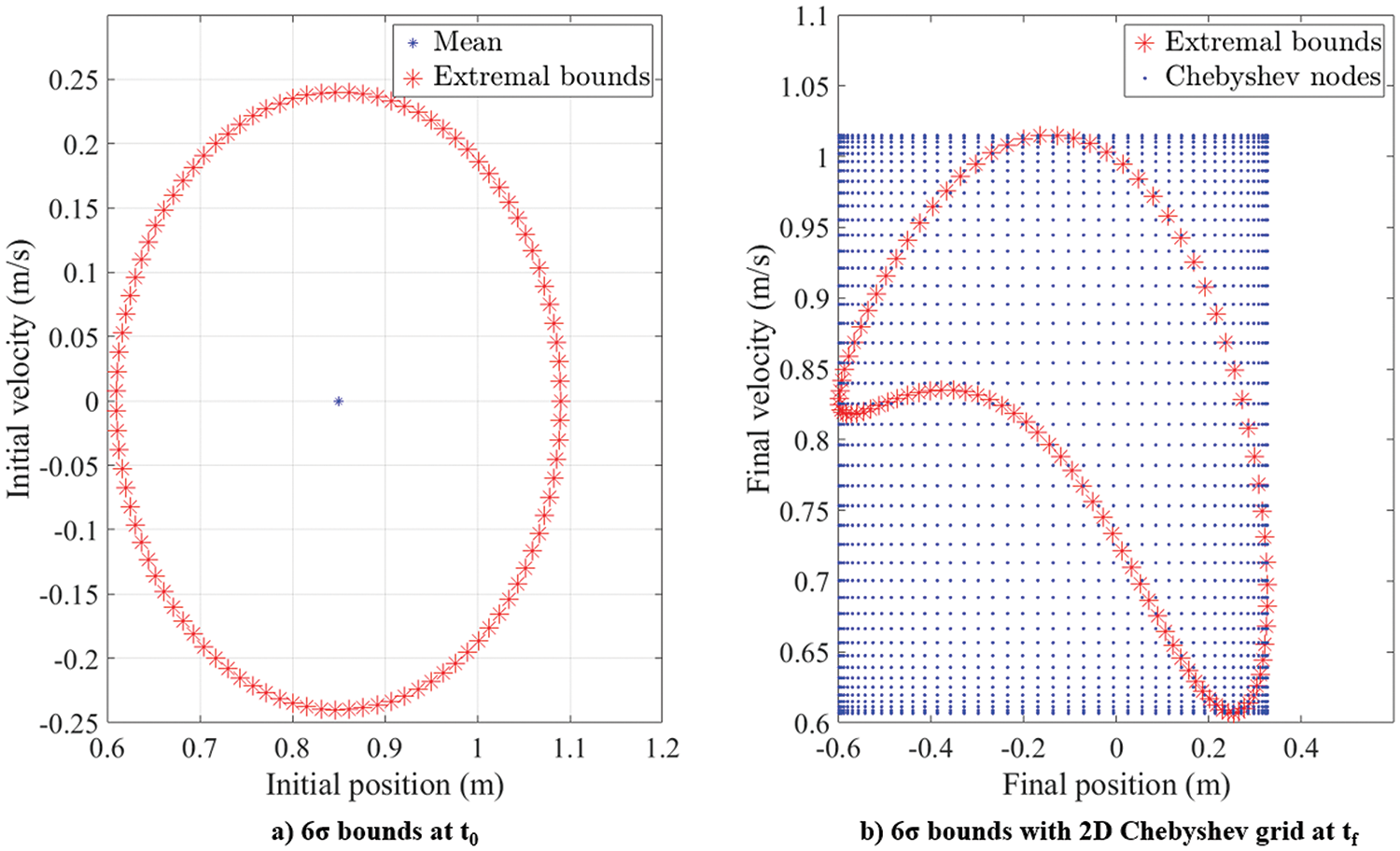
Figure 12: 2D conservative Duffing oscillator: bounds at t0 and tf

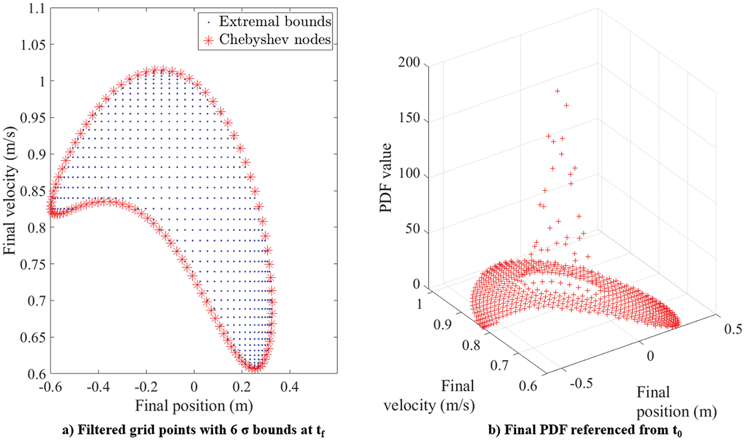
Figure 13: 2D conservative Duffing oscillator: filtered grid and referenced PDF at tf

From the computation point of view, the back-propagation process is the most time-consuming section of OPA. The time required for the back-propagation depends on three factors: i) the number of points that lie within the extremal bounds, ii) the initial and the final time (i.e., time span) of the back-propagation and iii) the complexity of the ODE system that is numerically integrated. After the back-propagation of each filtered grid point to t0, the corresponding PDF value is referenced to tf (Fig. 13). Then, the approximation is done using the Chebfun package to result in the PDF shown in Fig. 14. As the dynamics of the system are no longer linear, the analytic linear error propagation theory cannot be used for validation. Hence, Monte Carlo simulation is performed with 1 million sample points and the corresponding PDF is obtained using the kernel density estimation function. Fig. 14 shows the PDF corresponding to the Monte Carlo simulation of 1 million evaluation points. Since the PDF is non-Gaussian, the total probability integral value, I, is used as the metric to evaluate the accuracy of the PDF approximation. This value should come close to the cumulative integral of the truncated probability density function at t0. Fig. 15 depicts the close agreement between the 1-dimensional marginal PDFs and the cumulative integral curves of OPA and MC simulations. Table 4 shows the cumulative integral value of the PDF and the corresponding computation time for the OPA and MC simulations. OPA is shown to achieve nearly more than 100 times speed-ups vs. Monte Carlo simulations, as shown in Table 4, where the speed-up is calculated using the computation time of OPA and MC simulations.

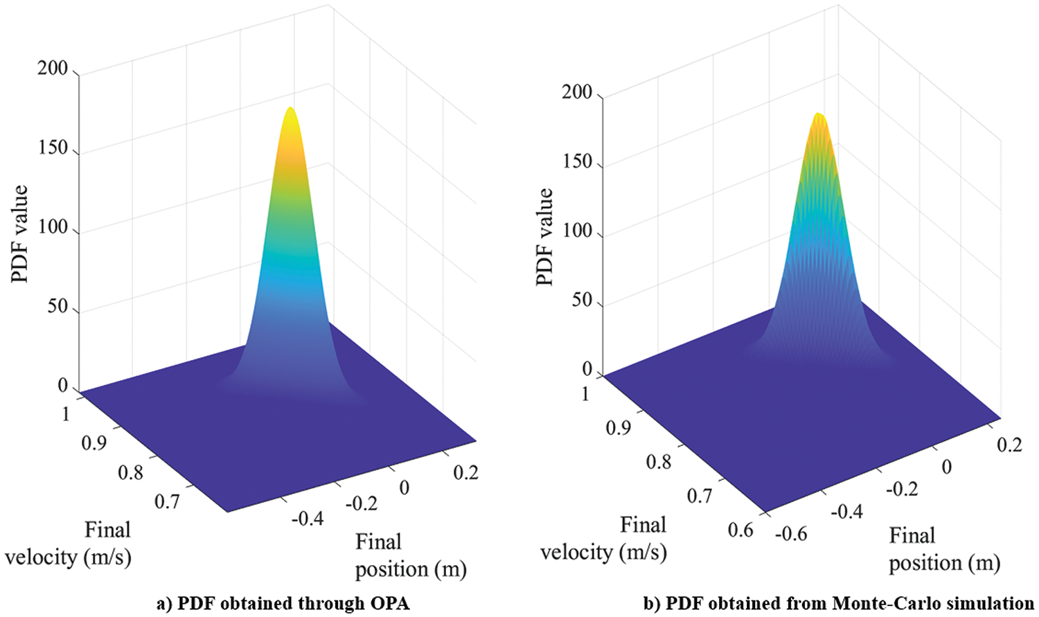
Figure 14: 2D conservative Duffing oscillator: PDFs from OPA and Monte Carlo simulation

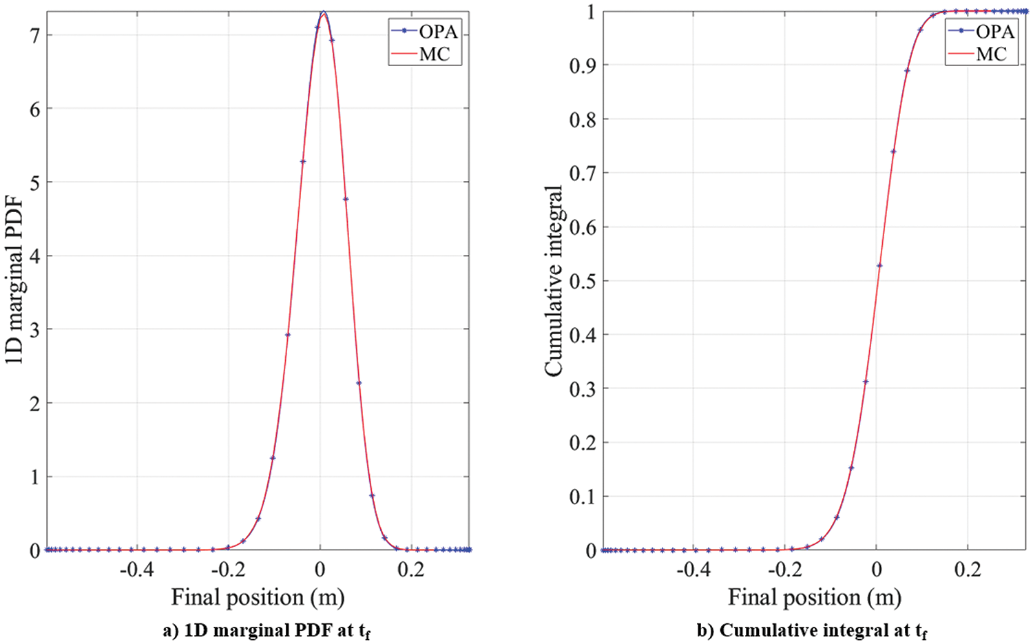
Figure 15: 2D conservative Duffing oscillator: comparison of the 1-dimensional marginal probability density function (PDF) and cumulative probability curves with MC simulation

3.2 The Damped Duffing Oscillator

In this section, OPA is applied to a damped Duffing oscillator with uncertainty in the damping coefficient, Eqs. (29) and (30). In this non-conservative dynamic system, the PDF at any given time depends on three random variables: (1) position, (2) velocity, and (3) the damping coefficient, δ. The state space trajectory of the oscillator is depicted in Fig. 16. The simulation parameters can be found in Tables 5 and 6. Since the problem has three random variables, it requires a 3-dimensional Chebyshev grid. Choosing an approximation order of n=28, results in n3 = 283 = 21,952 Chebyshev grid points before grid filtering.

x¨+δx˙+(1+k2)x−2k2x3=0(29)

δ˙=0(30)

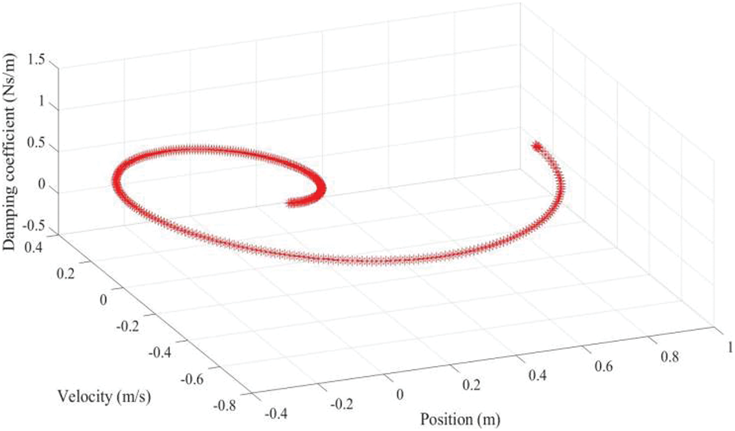
Figure 16: 3D non-conservative Duffing oscillator: state space propagation from t0 to tf

The stiffness coefficient k is treated as a constant, and the damping coefficient δ becomes the random variable whose variation with time is zero. Out of the 3 random variables in this problem, only position and velocity change with time. Fig. 17 shows the initial extremal bounds that are propagated to a final time tf using Eqs. (29) and (30) to obtain the final extremal bounds. As shown in Fig. 17, a 3-dimensional (3D) Chebyshev grid is then formed at the final time. Following the technique discussed in Section 2, the grid points within the final extremal bounds, Fig. 17, are filtered and then back-propagated. Because of the non-conservative nature of the system dynamics, the PDF values at the grid points referenced from the back-propagation need to be scaled before the approximation is done. Although the procedure described in Section 2.2 can be used to scale the backpropagated PDF values, there is a simple and efficient way to scale the PDF using the fact that the damping coefficient does not change with time in this simulation, δ˙=0. Using the nature of the Chebyshev grid, the selected grid points at tf can be grouped into several levels with each level defined by a constant value of δ (Fig. 18). A convex hull is formed using the grid points between two successive levels at tf. The volume of this convex hull is denoted as Vfi. Upon back-propagation, each grid point from a damping coefficient level at tf lands at different position and velocity coordinates at t0 but the value of the damping coefficient remains unchanged. A second convex hull is formed using the backpropagated grid points of the corresponding successive levels at t0, whose volume is termed as V0i. The convex hulls with volumes Vfi and V0i are shown in Fig. 19. The scale factor associated with this pair of levels is given by,

SFpairi=V0iVfi(31)

SFleveli=SFpairi+1+SFpairi2(32)

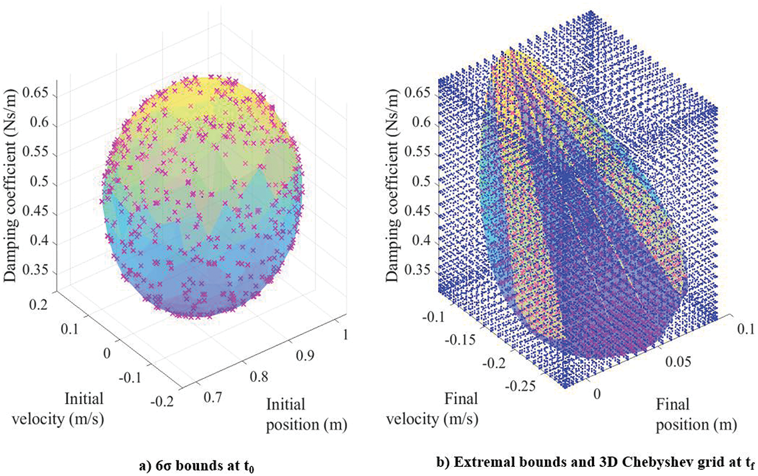
Figure 17: 3D non-conservative Duffing oscillator: initial and final bounds

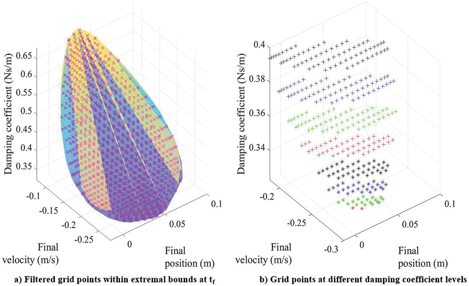
Figure 18: 3D non-conservative Duffing oscillator: filtered grid points and damping coefficient levels at tf (each colored layer of points (right) is a damping coefficient level with constant value for the damping coefficient)

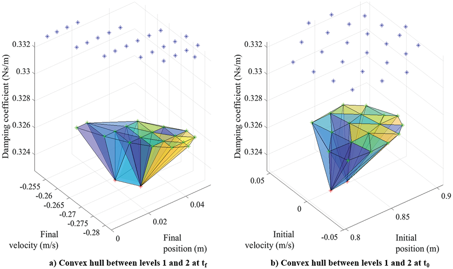
Figure 19: 3D non-conservative Duffing oscillator: PDF modulation using volume approximation

This process continues for each pair of successive levels until all the selected grid points are covered. For example, if there are 25 levels, then this method yields 24 scale factors. Since each level of grid points is paired with the level above and with the level below, the scale factor of that level is obtained by computing the average as shown in Eq. (32). This mean scale factor is then used to scale the referenced PDF values of that level. The procedure continues until the referenced PDF at all levels is scaled. After scaling, the 3D PDF is approximated using the Chebfun toolbox. Figs. 20 and 21 show the outcomes of integrating the approximated PDF with respect to one random variable at a time (i.e., damping coefficient and velocity, respectively). The sequence of integration is described in Eqs. (33) and (34),

g(x,x˙)=∫c1c2f(x,x˙,δ)dδ(33)

h(x)=∫x1˙x2˙g(x,x˙)dx˙(34)

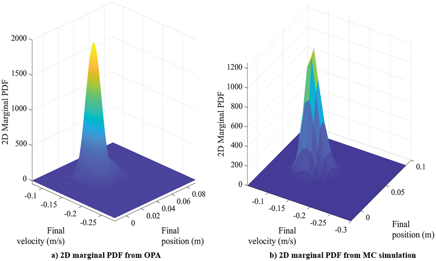
Figure 20: 3D non-conservative Duffing oscillator: comparison of 2D marginal PDFs

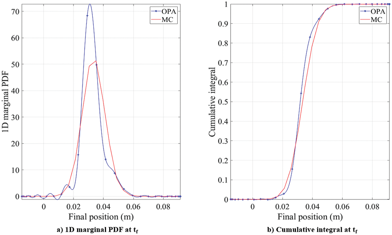
Figure 21: 3D non-conservative Duffing oscillator: comparison of the 1-dimensional marginal probability density function (PDF) and cumulative integral curves with MC simulation

The smoothness of the cumulative probability curve depends on the order of approximation used. In the 2D Duffing oscillator problem, Table 4 shows that an MC simulation with 1 million points is required to achieve a reasonably accurate cumulative integral value. Therefore, using 1 million points, Fig. 20, an MC simulation is used to validate the approximation process. Table 7 shows that both the OPA and Monte Carlo simulations yield cumulative integral values close to one (to three decimal places). However, OPA is more than 270 times faster than the conventional Monte Carlo approach.

3.3 The Planar Orbit Problem

A higher-dimensional application of OPA is propagating the PDF of a simulated orbit problem. When using Chebyshev polynomials for higher dimensions, it becomes computationally expensive to compute full multi-dimensional approximations for the PDF. Additionally, for most real-world problems, only the spatial dimensions are required for further computations. This means that a one-dimensional approximation can be used to integrate the non-spatial dimensions of the PDF so that only a 2D or 3D Chebyshev approximation is required. This is achieved by selecting a dimension for integration and then, for each of the combinations of the non-selected dimensions, integrating along a one-dimensional line of the selected dimension to compress its probability into a single point in a space defined by the non-selected dimensions. This process is then repeated for all non-spatial dimensions. A simple LEO planar orbit problem is considered with uncertainty in the initial position and velocity. Because of the nature of the coupled dynamics, the PDF becomes a function of four random variables: position (x, y) and velocity (Vx=x˙, Vy=y˙). In this problem with two spatial and two velocity dimensions, at each constant value of x, y, and x˙, a one-dimensional integral along y˙ will compress the 4D space into a 3D space. Repeating this along x˙ compresses the space to 2D, and then a 2D Chebyshev approximation can be used for the spatial dimensions.

The state vector for the planar orbit problem is written as,

X=[xyx˙y˙]T(35)

X˙=[x˙y˙x¨y¨]T(36)

x¨=−µer3x(37)

y¨=−µer3y(38)

r=x2+y2(39)

Tables 8 and 9 present the orbital elements and other relevant parameters of the planar orbit chosen to demonstrate OPA, respectively. The 6σ initial extremal bound of the planar orbit problem is defined by 500 points, which are obtained using the initial values of the uncertainties for the four random variables given in Table 10 and the procedure described in Section 2.4. These points, with a constant value of the PDF, are shown in Fig. 22. Since there are four random variables, the 4D extremal bounds are shown in two separate plots. Upon propagating these extremal bounds to one-fourth (= 0.25 * T) of the period of the orbit, the final extremal bounds are obtained, as shown in Fig. 23. A 4D Chebyshev grid encompassing the final extremal bounds is then formed (Fig. 24), and the points within the extremal bounds are filtered (Fig. 25) using the procedure mentioned in Section 2.3. These points are backpropagated to t0 (Fig. 26), and the PDF value at each (x0, y0, x˙0, y˙0) is referenced to tf.

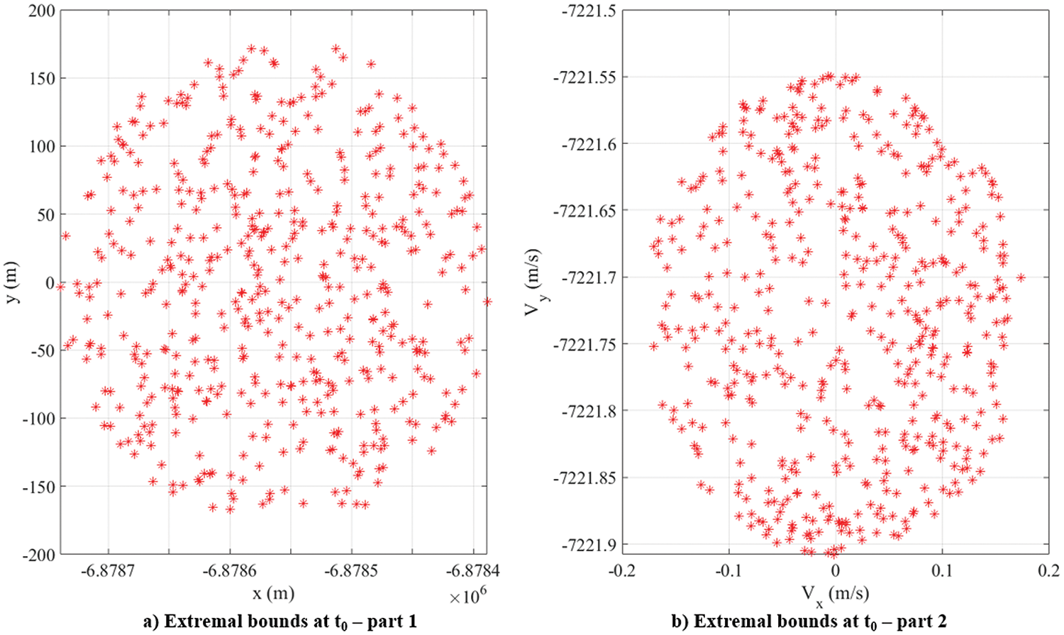
Figure 22: Planar orbit: 6σ extremal bound points at t0

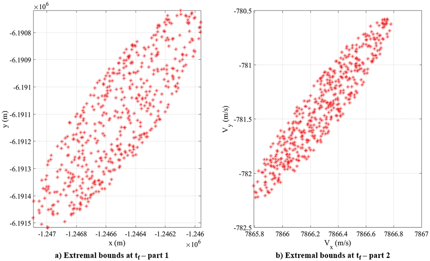
Figure 23: Planar orbit: 6σ extremal bound points at tf

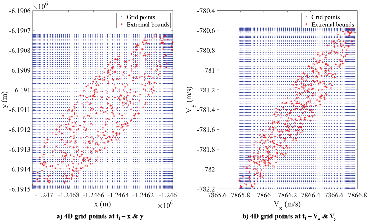
Figure 24: Planar orbit: extremal bounds with 4D Chebyshev grid at tf

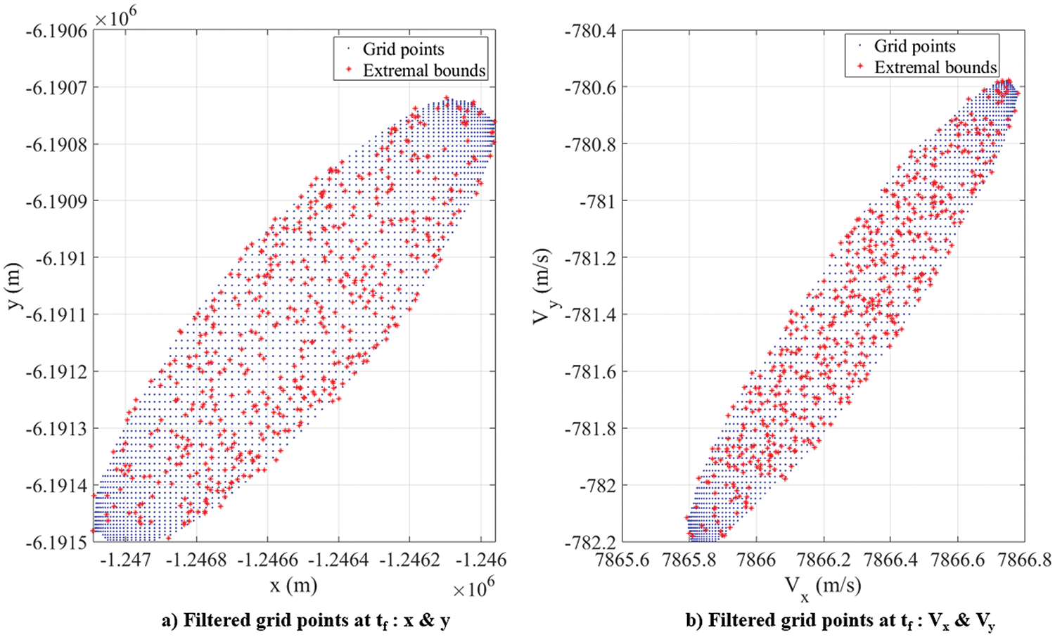
Figure 25: Planar orbit: filtered 4D Chebyshev grid points at tf

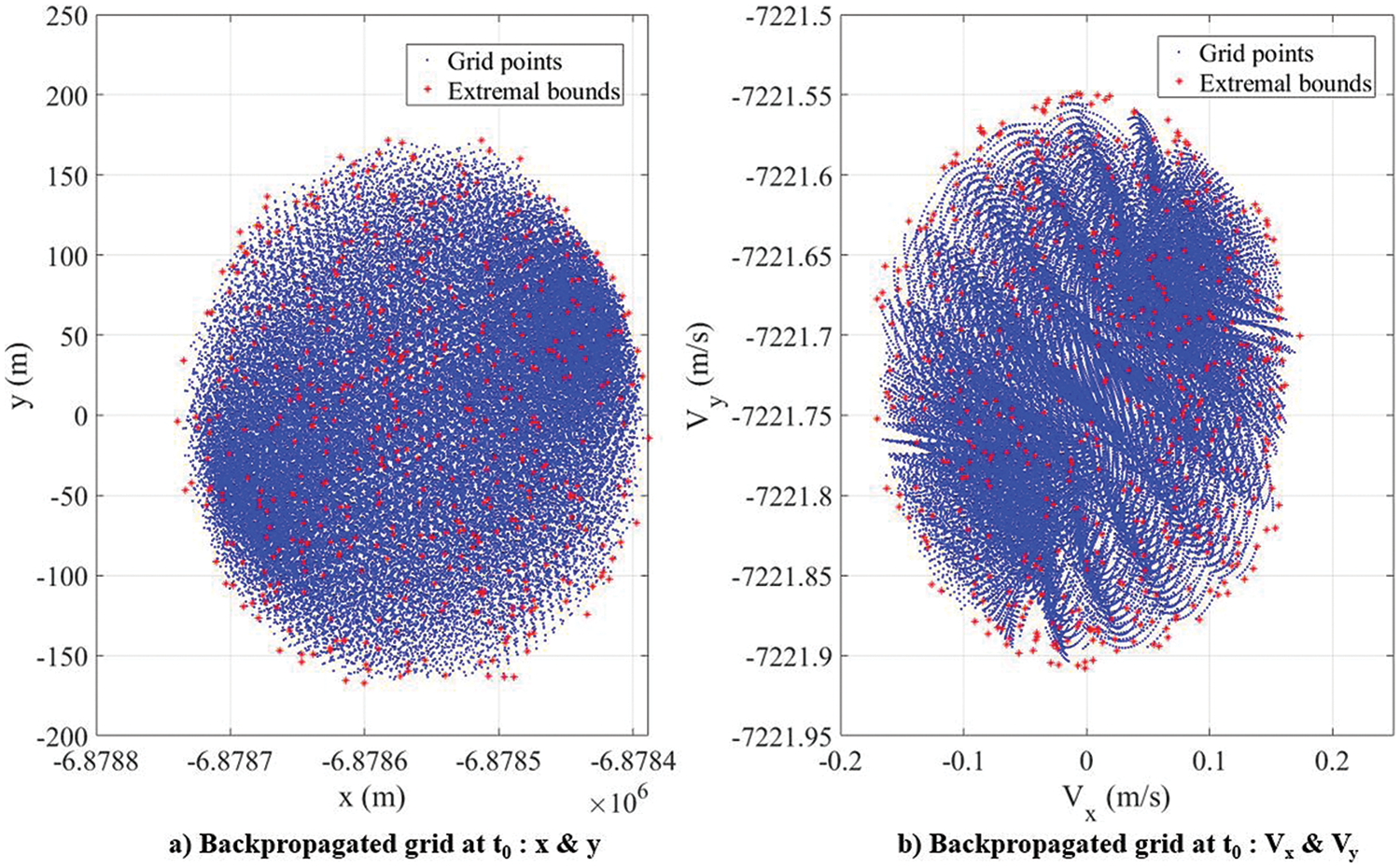
Figure 26: Planar orbit: filtered grid points after back-propagation at t0

Although the number of grid points increases exponentially with the dimensionality of the problem, grid filtering makes the back-propagation tractable. From Table 10, the ratio of the standard deviations of the spatial and velocity dimensions is found to be 30/0.03 = 1000. From numerical experiments, it was found that maintaining the ratio around this value results in enough backpropagated grid points within the extremal bounds, which ensures a good-quality approximation of the PDF at tf. The 4D PDF is then approximated using the higher-dimensional approximation procedure described above. After approximation, a 2D and a 1D marginal PDF are obtained by the integration sequence given in Eqs. (30)–(32). Finally, the cumulative integral is also obtained by integrating the 1D marginal PDF with respect to the x position.

f2(x,y,x˙)=∫y1˙y2˙f1(x,y,x˙,y˙)dy˙(40)

f3(x,y)=∫x1˙x2˙f2(x,y,x˙)dx˙(41)

f4(x)=∫y1y2f3(x,y)dy(42)

The equivalent 2D and 1D marginal PDFs, as well as the cumulative integral curves from a 1 million Monte Carlo simulation of the planar orbit problem, are also obtained by following the integration sequence given above. These comparisons can be seen in Figs. 27 and 28.

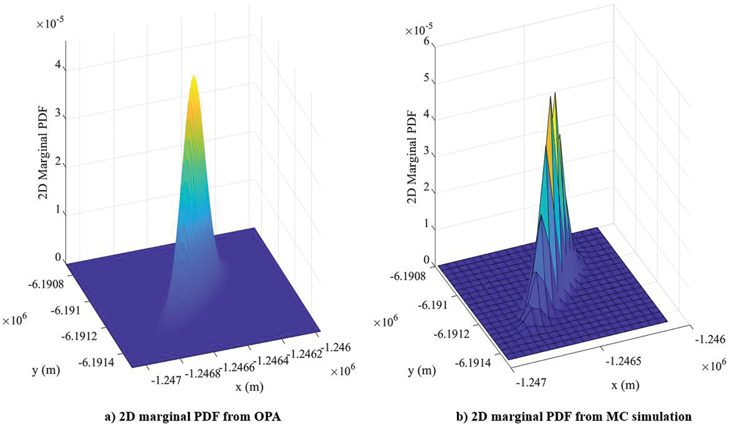
Figure 27: Planar orbit: 2D marginal PDFs from OPA and MC simulation

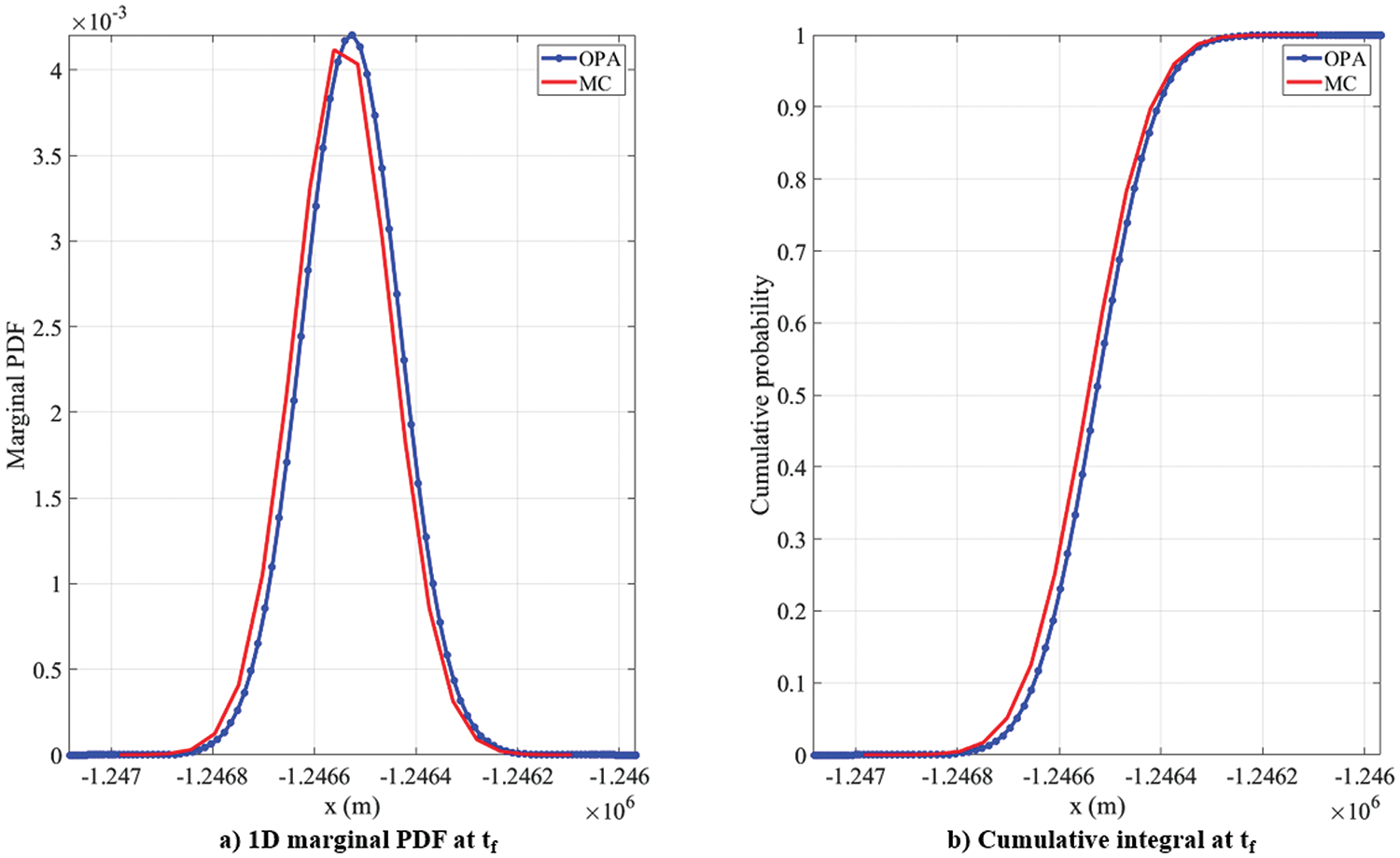
Figure 28: Planar orbit: comparison of 1D marginal PDF and cumulative integral curves from OPA and MC simulation

The smoothness of the curve and convergence of the cumulative integral value to one indicates the quality of the PDF approximation. Several trials of OPA with different approximation orders were run, and the outcomes are summarized in Table 11. The speed-up is obtained by considering the one million sample Monte Carlo simulation as a reference. Fig. 29 shows the plots of the error in the cumulative integral value and speed up with the approximation order. For the approximation order of 90, the cumulative integral value is comparable to that of the MC simulation, and the OPA simulation is at least eight times faster than the MC simulation. Although the computation time will vary according to the hardware architecture on which the simulation is performed, the speed up will remain constant. This shows the accuracy, efficiency, and reliability of OPA for approximating the PDF of the planar orbit problem.

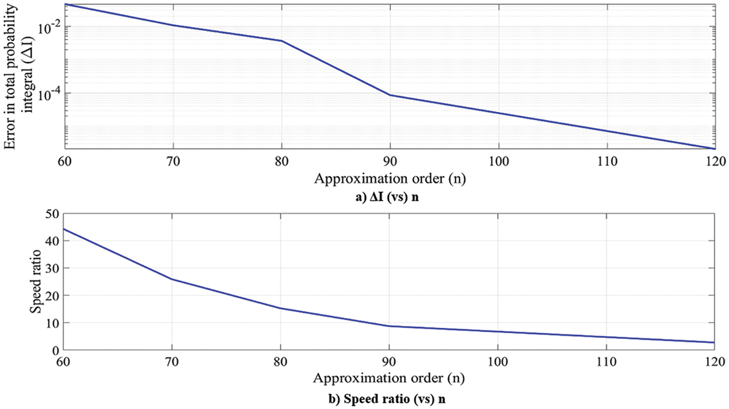
Figure 29: Planar orbit problem: OPA performance-speed up and total integral accuracy

4  Discussion

Results presented in Section 3 show OPA to achieve nearly the same PDF approximation accuracy as seen in Monte Carlo simulations but with superior computational efficiency. In the case of the 2D conservative Duffing oscillator, the PDF approximation using OPA requires almost three orders of magnitude fewer grid points than that of the Monte Carlo simulation while being more than 100 times faster. For the non-conservative Duffing oscillator problem, OPA again requires almost three orders of magnitude fewer grid points while being more than 270 times faster than the corresponding Monte Carlo simulation. Finally, in the planar orbit problem, the best case of OPA requires two orders of magnitude fewer points while being 8 times faster than the corresponding MC simulation.

While both OPA and non-intrusive polynomial chaos use stochastic collocation, OPA quantifies the system uncertainty at the final time by directly approximating the higher-dimensional PDF surface. On the other hand, non-intrusive polynomial chaos approximates each random variable of the system using polynomials that are, in turn, functions of other standard random variables. OPA employs targeted sampling by exploiting the geometry of the future PDF. In other words, by utilizing the shape of the future PDF, OPA uses only those samples that contribute to the PDF approximation [23,26].

The grid filtering scheme described in this paper fits a convex hull over the points on the 6σ extremal bounds. For more concavely shaped extremal bounds, like the classic banana shape, this scheme will lead to fewer internal grid points after filtering. This will be addressed in future works using better algorithms to improve the accuracy of grid filtering. For the initial uncertainties, the examples presented in this paper utilize a Gaussian distribution because it is the most common error distribution in the outcomes of estimation/filtering schemes like the Extended Kalman Filter (EKF). In general, OPA can be used to approximate the non-Gaussian PDF in a filtering scheme in which the system’s observations are not available for extended periods due to situations like occultation by the Earth, e.g., space debris on the far side of the Earth [42]. Under such circumstances, the initial uncertainties of the object, obtained from the last observed/known epoch in the filtering/estimation scheme, are usually Gaussian. The functional description of the non-Gaussian PDF provided by OPA at the final time can be used as the initial condition for uncertainty propagation in the subsequent period. Hence, without loss of generality, OPA can be used to propagate the uncertainties of a dynamic system when the initial distribution is known.

5  Conclusion and Future Work

High-fidelity uncertainty propagation is a challenging area of research, especially in situations involving space assets. Orthogonal Polynomial Approximation (OPA) proves to be an excellent candidate for high-quality Probability Density Function (PDF) approximations. The methodology of OPA is concisely explained with a one-dimensional conceptual example, followed by the procedure to implement OPA for non-conservative systems. PDF modulation and scaling are illustrated for a two-dimensional case. Issues concerning back-propagation are described, followed by an illustration of grid filtering. A simple harmonic oscillator is used as a case for linear system validation. Results show an excellent match between the PDFs obtained from OPA and analytic linear error propagation theory.

The proposed method is then applied to three different nonlinear systems: 1) a conservative Duffing oscillator, 2) a Duffing oscillator with damping coefficient uncertainty, and 3) a planar orbit problem in Low Earth Orbit (LEO). Through one million sample Monte Carlo simulations, the uncertainty propagation in all three nonlinear systems has been validated. For all the cases shown in the paper, OPA is more computationally efficient than Monte Carlo simulation.

Using the cumulative integral as an accuracy metric for PDF approximation quality is necessary but insufficient. Future research in this direction will utilize other statistical indicators such as entropy and Kullback-Leibler (KL) divergence to compare the PDFs. Moreover, when the propagation time of the planar orbit problem is increased beyond 0.25 T, the extremal bounds become narrower and more slender. This reduces the number of grid points that lie within the extremal bounds, which in turn decreases the quality of the approximated PDF. This problem can be overcome by using segmented or local basis functions, which future works will explore. Further studies will investigate the application of OPA to obtain collision probability in nonlinear systems.

Acknowledgement: Besides the funding provided by Lockheed Martin Space, the authors would like to acknowledge the compute resources provided by the University of Central Florida.

Funding Statement: The authors of this study would like to express their gratitude for the funding provided by Lockheed Martin Space-University collaboration.

Author Contributions: The authors confirm contribution to the paper as follows: Study conception and design: Tarek A. Elgohary, Austin B. Probe; Simulations design, execution, and result generation: Pugazhenthi Sivasankar; Analysis and interpretation of results: Tarek A. Elgohary, Austin B. Probe, Pugazhenthi Sivasankar; Draft manuscript preparation: Pugazhenthi Sivasankar, Tarek A. Elgohary. All authors reviewed the results and approved the final version of the manuscript.

Availability of Data and Materials: All the data used for the simulations in this article can be recreated using the specific conditions/statistical parameters mentioned in the respective sections. No external data from any sensor has been used in this study.

Ethics Approval: Not applicable.

Conflicts of Interest: The authors declare no conflicts of interest to report regarding the present study.

References

1. D. Vallado, “Mission analysis,” in Fundamentals of Astrodynamics and Applications, 4 ed. Hawthrone, CA, USA: Space Technology Library, 2013, vol. 1, pp. 837–845. Accessed: Feb. 12, 2023. [Online]. Available: https://www.amazon.com/Fundamentals-Astrodynamics-Applications-Technology-Library/dp/1881883183 [Google Scholar]

2. S. Alfano, “Satellite conjunction Monte-Carlo analysis,” Adv. Astronaut. Sci., vol. 134, no. 1, pp. 2007–2024, Feb. 2009. [Google Scholar]

3. J. Carpenter, “Non-parametric collision probability for low-velocity encounters,” presented at the 17th AAS/AIAA Spaceflight Mech., Mtng, Sedona, AZ, USA, Jan. 28–Feb. 1, 2007, AAS-07-201. [Google Scholar]

4. F. Chan, “Spacecraft encounters,” in Spacecraft Collision Probability, 1 ed. El Segundo, CA, USA: The Aerospace Press, 2008, vol. 1, pp. 15–27. Accessed: Jan. 20, 2023. [Online]. Available: https://www.semanticscholar.org/paper/Spacecraft-Collision-Probability-Chan/dc63d94240888414f20ab64a39841e63806caf17 [Google Scholar]

5. J. Junkins, M. Akella, and K. Alfriend, “Non-gaussian error propagation in orbital mechanics,” J. Astronaut. Sci., vol. 44, no. 1, pp. 541–563, Oct. 1996. [Google Scholar]

6. A. Probe, T. Elgohary, and J. Junkins, “A new method for space objects probability of collision,” presented at the AIAA/AAS Astrodynamics Specialist Conf., Longbeach, CA, USA, Sep. 13–16, 2016, AIAA 2016-5653. [Google Scholar]

7. M. Akella and K. Alfriend, “Probability of collision between space objects,” J. Guid. Control Dyn., vol. 23, no. 5, pp. 769–772, Oct. 2000. doi: 10.2514/2.4611. [Google Scholar]

8. M. Majji, J. Junkins, and J. Turner, “A high order method for estimation of dynamic systems,” J. Astronaut. Sci., vol. 56, no. 3, pp. 401–440, Sep. 2008. doi: 10.1007/BF03256560. [Google Scholar]

9. K. Fujimoto, D. Scheeres, and K. Alfriend, “Analytical nonlinear propagation of uncertainty in the two-body problem,” J. Guid. Control Dyn., vol. 35, no. 2, pp. 497–509, Apr. 2012. doi: 10.2514/1.54385. [Google Scholar]

10. T. Tasif and T. Elgohary, “An adaptive analytic continuation technique for the computation of the higher order state transition tensors for the perturbed two-body problem,” presented at the AIAA Scitech, Orlando, FL, USA, Jan. 6–10, 2020, AIAA 2020-0958. [Google Scholar]

11. T. Tasif and T. Elgohary, “An adaptive analytic continuation method for computing the perturbed two-body problem state transition matrix,” J. Astronaut. Sci., vol. 67, no. 4, pp. 1412–1444, Nov. 2020. doi: 10.1007/s40295-020-00238-9. [Google Scholar]

12. T. Tasif, Adaptive Analytic Continuation for the State Transition Tensors of the Two-Body Problem. Orlando, FL, USA: University of Central Florida, 2022. [Google Scholar]

13. S. Boone and J. McMahon, “Directional state transition tensors for capturing dominant nonlinear effects in orbital dynamics,” J. Guid. Control Dyn., vol. 46, no. 3, pp. 431–442, Nov. 2022. doi: 10.2514/1.G006910. [Google Scholar]

14. D. Qiao, X. Zhou, and X. Li, “Feasible domain analysis of heliocentric gravitational-wave detection configuration using semi-analytical uncertainty propagation,” Adv. Space Res., vol. 72, no. 10, pp. 4115–4131, Nov. 2023. doi: 10.1016/j.asr.2023.08.011. [Google Scholar]

15. R. Armellin, P. Di Lizia, F. Bernelli-Zazzera, and M. Berz, “Asteroid close encounters characterization using differential algebra: The case of Apophis,” Celest. Mech. Dyn. Astron., vol. 107, no. 4, pp. 451–470, Jun. 2010. doi: 10.1007/s10569-010-9283-5. [Google Scholar]

16. M. Valli, R. Armellin, P. Di Lizia, and M. Lavagna, “Nonlinear mapping of uncertainties in celestial mechanics,” J. Guid. Control Dyn., vol. 36, no. 1, pp. 48–63, Dec. 2012. doi: 10.2514/1.58068. [Google Scholar]

17. C. Sabol, C. Binz, A. Segerman, K. Roe, and P. J. Schumacher, “Probability of collision with special perturbations dynamics using the Monte-Carlo method,” presented at the AIAA/AAS Astrodyn. Specialist Conf., Girdwood, AK, USA, Jul. 31–Aug. 4, 2011, AAS 11-435, AAS 11-435. [Google Scholar]

18. D. Hall, S. Casali, L. Johnson, B. Skrehart, and L. Baars, “High-fidelity collision probabilities estimated using brute force Monte-Carlo simulations,” presented at the AIAA/AAS Astrodyn. Specialist Conf., Snowbird, UT, USA, Aug 19–23, 2018, AAS 18-244. [Google Scholar]

19. G. Terejanu, P. Singla, T. Singh, and P. Scott, “Uncertainty propagation for nonlinear dynamic systems using Gaussian mixture models,” J. Guid. Control Dyn., vol. 31, no. 6, pp. 1623–1633, Dec. 2008. doi: 10.2514/1.36247. [Google Scholar]

20. B. Grace and J. McMahon, “Application of gaussian mixture models for nonlinear uncertainty propagation during martian aerocapture,” presented at the AAS/AIAA Astrodyn. Specialist Conf., Lake Tahoe, CA, USA, Aug. 9–12, 2020, AAS 20-485. [Google Scholar]

21. Z. Sun, Y. Luo, P. Di Lizia, and F. Zazzera, “Nonlinear orbital uncertainty propagation with differential algebra and Gaussian mixture model,” Sci. China-Phy. Mech. Astron., vol. 62, no. 3, pp. 1–11, Mar. 2019. doi: 10.1007/s11433-018-9267-6. [Google Scholar]

22. H. Xie, T. Xue, W. Xu, G. Liu, H. Sun and S. Sun, “Orbital uncertainty propagation based on adaptive gaussian mixture model under generalized equinoctial orbital elements,” Remote Sens., vol. 15, no. 19, Sep. 2023, Art. no. 4652. doi: 10.3390/rs15194652. [Google Scholar]

23. B. Jones, A. Doostan, and G. Born, “Nonlinear propagation of orbit uncertainty using non-intrusive polynomial chaos,” J. Guid. Control Dyn., vol. 36, no. 2, pp. 430–444, Apr. 2013. doi: 10.2514/1.57599. [Google Scholar]

24. R. Bhusal and K. Subbarao, “Generalized polynomial chaos expansion approach for uncertainty quantification in small satellite orbital debris problems,” J. Astronaut. Sci., vol. 67, no. 1, pp. 225–-253, Mar. 2020. doi: 10.1007/s40295-019-00176-1. [Google Scholar]

25. X. iang, S. Li, R. Furfaro, Z. Wang, and Y. Ji, “High-dimensional uncertainty quantification for Mars atmospheric entry using adaptive generalized polynomial chaos,” Aerosp. Sci. Technol., vol. 107, no. 1, Dec. 2020, Art. no. 106240. doi: 10.1016/j.ast.2020.106240. [Google Scholar]

26. B. Jia and M. Xin, “Short-arc orbital uncertainty propagation with arbitrary polynomial chaos and admissible region,” J. Guid. Control Dyn., vol. 43, no. 4, pp. 715–728, Apr. 2020. doi: 10.2514/1.G004548. [Google Scholar]

27. Y. Sun and M. Kumar, “Numerical solution of high dimensional stationary Fokker-Planck equations via tensor decomposition and Chebyshev spectral differentiation,” Comput. Math. App., vol. 67, no. 10, pp. 1960–1977, Jun. 2014. doi: 10.1016/j.camwa.2014.04.017. [Google Scholar]

28. A. Chertkov and I. Oseledets, “Solution of the Fokker-Planck equation by cross approximation method in the tensor train format,” Front. Artif. Intell., vol. 4, no. 1, Aug. 2021, Art. no. 668215. doi: 10.3389/frai.2021.668215. [Google Scholar]

29. C. T. Shelton and J. Junkins, “Probability of collision between space objects including model uncertainty,” Acta Astronaut., vol. 155, no. 1, pp. 462–471, Feb. 2019. doi: 10.1016/j.actaastro.2018.11.051. [Google Scholar]

30. M. Torky, A. Hassanein, A. El Fiky, and Y. Alsbou, “Analyzing space debris flux and predicting satellites collision probability in LEO orbits based on petri nets,” IEEE Access, vol. 7, no. 1, pp. 83461–83473, Jun. 2019. doi: 10.1109/ACCESS.2019.2922835. [Google Scholar]

31. X. Zhou, D. Qiao, and X. Li, “Neural network-based method for orbit uncertainty propagation and estimation,” IEEE Trans. Aerosp. Electron. Syst., vol. 60, no. 1, pp. 1176–1193, Nov. 2023. doi: 10.1109/TAES.2023.3332566. [Google Scholar]

32. P. Singla and J. Junkins, “Global local orthogonal polynomial MAPping (GLO-MAP) in N dimensions,” in Multi-Resolution Methods for Modeling and Control of Dynamical Systems, 1 ed. New York, NY, USA: Chapman and Hall/CRC, 2008, vol. 1, pp. 123–174. Accessed: Apr. 22, 2023. [Online]. Available: https://www.taylorfrancis.com/books/mono/10.1201/9781584887706/multi-resolution-methods-modeling-control-dynamical-systems-puneet-singla-john-junkins [Google Scholar]

33. M. Mercurio, R. Mandankan, P. Singla, and M. Majji, “Approximation of probability density functions propagated through the perturbed two-body problem,” presented at the AIAA/AAS Astrodyn. Specialist Conf., Hilton Head, SC, USA, Aug. 11–15, 201. [Google Scholar]

34. A. Probe, C. Shelton, T. Elgohary, and J. Junkins, “Orbital probability of collision using orthogonal polynomial approximations,” presented at the 1st IAA Conf. Space Situat. Awareness, Orlando, FL, USA, Nov. 13–15, 2017, IAA-ICSSA-17-06-34. [Google Scholar]

35. P. Sivasankar, B. Lewis Jr, A. Probe, and T. Elgohary, “Validation of orthogonal probability approximation for space situational awareness using real satellite data,” presented at the 3rd IAA Conf. Space Situat. Awareness, Madrid, Spain, Apr. 4–6, 2022, IAA-ICSSA-22-0015. [Google Scholar]

36. B. Hashemi and L. Trefethen, “Chebfun in three dimensions,” SIAM J. Sci. Comput., vol. 39, no. 5, pp. C341–C363, Sep. 2017. doi: 10.1137/16M1083803. [Google Scholar]

37. J. Gibbs, “On the fundamental formula of statistical mechanics, with applications to astronomy and thermodynamics,” in The Collected Works of J. Willard Gibbs, 1 ed. London, England: Longmans & Green, 1931, vol. 2, pp. 220–225. Accessed: Aug. 20, 2022. [Online]. Available: https://www.amazon.com/Collected-Works-Willard-Gibbs-Volumes/dp/B000V7FQTW [Google Scholar]

38. Y. Luo and Z. Yang, “A review of uncertainty propagation in orbital mechanics,” Prog. Aerospace Sci., vol. 89, no. 1, pp. 23–39, Feb. 2017. doi: 10.1016/j.paerosci.2016.12.002. [Google Scholar]

39. J. D’Errico, “Inhull,” MATLAB Central File Exchange. Accessed: Oct. 11, 2024. [Online]. Available: https://www.mathworks.com/matlabcentral/fileexchange/10226-inhull [Google Scholar]

40. J. Crassidis and J. Junkins, “Sequential state estimation,” in Optimal Estimation of Dynamic Systems, 2 ed. Boca Raton, FL, USA: Chapman and Hall/CRC, 2012, vol. 2, pp. 135–202. Accessed: May 30, 2023. [Online]. Available: https://ancs.eng.buffalo.edu/index.php/Optimal_Estimation_of_Dynamic_Systems_2nd_Ed [Google Scholar]

41. N. Hale and L. Trefethen, “Chebfun and numerical quadrature,” Sci. China Math., vol. 55, no. 9, pp. 1749–1760, Jul. 2012. doi: 10.1007/s11425-012-4474-z. [Google Scholar]

42. T. Tasif, J. Hippelheuser, and T. Elgohary, “Analytic continuation extended Kalman filter framework for perturbed orbit estimation using a network of space-based observers with angles-only measurements,” Astrodyn, vol. 6, no. 2, pp. 161–187, May 2022. doi: 10.1007/s42064-022-0138-0. [Google Scholar]

Appendix A