Research on AC Electronic Load with Energy Recovery Based on Finite Control Set Model Predictive Control

1  Introduction

With the development of new energy field, more and more electrical equipment based on power converters has been put into engineering practice. The realization of stable power supply of electrical equipment is of urgently required to new energy development at this stage [1]. Uninterruptible power supplies, the current main power supply equipment, have been widely used in various industrial production fields [2]. In order to ensure the stability of its power supply, a long-term aging test and input characteristic test must be strictly carried out before filed application [3,4]. Conventional loads generate a large amount of heat loss during their use, which results in wasted energy and shortens the load life. Therefore, conventional loads are not suitable for long-term power supply testing. The development of new power supply test device becomes very urgent. With the advent of AC electronic loads, the issues mentioned above can be solved.

AC electronic load is an alternative power electronic device. According to the four-quadrant operating characteristics of the PWM rectifier, it can simulate various characteristic loads and effectively replace the traditional load to complete the power supply test. By adding a grid-connected inverter to the original AC electronic load, the energy generated by the test can be fed back to the grid [5].

The AC electronic load with energy recovery generally adopts the back-to-back topology of the voltage source PWM rectifier. The control goal of the front stage is to track the reference current, and the control goal of the rear stage is usually to stabilize the DC link voltage as well as unity power factor grid connection [6]. At present, the more commonly used control strategies are hysteresis current control [7], space vector control (SVPWM) [8], etc. However, the hysteresis current control current has more harmonic contents, and the SVPWM vector control table is much more complicated. Considering the development of digital signal processors in recent years, some advanced control algorithms with high computing power can be put into engineering practice. This makes these algorithms have some expected performance in the control of the AC electronic load with energy recovery.

FCS-MPC is a popular control algorithm in the control of power electronics. FCS-MPC has been proven a simple and effective alternative to the traditional PWM control algorithm in [9,10], and it has a good performance in the control of power converters [11]. In [12], the author gives a detailed guideline about the design of FCS-MPC controllers. In order to control the currents under unbalanced load and supply condition, Gulbudak et al. [13] presents a control strategy for dual-output four-leg Indirect Matrix Converter. In [14], the author proposed a novel model predictive control strategy for the three-phase Direct Matrix Converter based on switching state elimination. To solving the problem of the weighting factors to multiple control goals, Gulbudak et al. [15,16] proposed a novel Lyapunov-based model predictive control strategy, it reformulated the cost function to Lyapunov energy function to ensure the stability. Babaie et al. [17] applied it to the control of Seven-Level Modified PUC Active Rectifier, and achieved a better control effect. To improving the robustness under the condition of unavoidable measuring noises and parameter variation, Wang et al. [18] proposed a passivity-based model predictive control, the control algorithm has similar characteristics to FCS-MPC.

However, due to some problems of FCS-MPC itself, such as large amount of system calculation and unstable switching frequency, it still faces many challenges in its future development [19].

In recent years, many scholars have conducted a series of studies on the calculation of FCS-MPC, analyzed and simplified from different directions, and obtained some more effective improvement schemes. In [20], the author proposed a method to reduce the computational burden of the system by transforming the predictions. Although it can effectively reduce the computational cost, it is only suitable for short prediction horizons. To solve the problem of long prediction horizons, Geyer et al. [21] proposed a multistep FCS-MPC with a modified sphere decoding algorithm, which solved this problem more effectively. For multilevel converters, a three-iteration simplified FCS-MPC has been proposed in [22], where only three states were evaluated in each iteration, which achieved good control results. A hierarchical FCS-MPC has been proposed in [23], the specific steps are as follows: for redundant vectors, two cost functions are set, and the optimal vector and redundant vector obtained by the calculation of the first cost function form the search pool of the second cost function, then obtain the optimal switching state through the calculation of the second cost function. In [24], the author reduced the computational cost by solving a quadratic programming problem, which was effectively improved without compromising the control performance. Due to the delay problem caused by the large amount of calculation of FCS-MPC, Gao et al. [25] proposed a compensation method by predicting the current variation within the delay time.

In this paper, considering the current state of control of AC electronic loads with energy recovery, FCS-MPC is introduced into its control. This paper compares and analyzes the control of traditional space vector control (SVPWM) and traditional FCS-MPC on AC electronic loads with energy recovery, and proves the feasibility of FCS-MPC. Under the condition of not affecting the control performance, the calculation amount of the system is greatly reduced by improving the original control strategy. This paper provides a new choice for the control of the AC electronic load in the future, and a more suitable control algorithm can be selected according to the actual situation.

2  Topology Structure and Control Strategy of AC Electronic Load

2.1 Topology Structure

At present, the research on the topology structure of the AC electronic load with energy recovery is relatively mature. Based on the topology structure proposed in [26], this paper selects a back-to-back voltage source three-phase PWM rectifier as the main circuit topology which is shown below in Fig. 1.

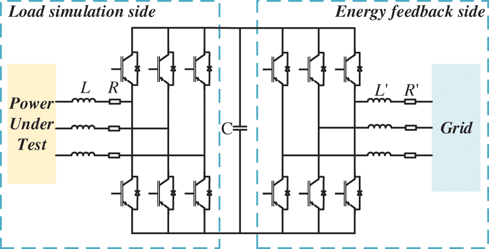
Figure 1: Topological structure of the AC electronic load with energy recovery

The front and rear stages of the AC electronic load can operate independently and are separated by a DC bus capacitor. In Fig. 1, L and L′ are the Filter inductor, R and R′ are the equivalent resistance, C is the DC bus capacitor. The front stage is the load simulation side, which realizes the simulation of various characteristic loads by controlling the input current. The rear stage is the energy feedback side, which realizes unity power factor grid connection by controlling the phase angle and amplitude of the grid-connected current.

2.2 System Control Strategy

2.2.1 Converter Model

The topology structure of the AC electronic load with energy recovery is symmetrical, a part of it can be chosen to establish and analyze a mathematical model. The AC electronic load is mainly composed of voltage source PWM rectifier. This paper chooses to directly study the mathematical model of the voltage source PWM rectifier to analyze the control strategy. A simplified circuit model of a voltage source PWM rectifier is shown in Fig. 2.

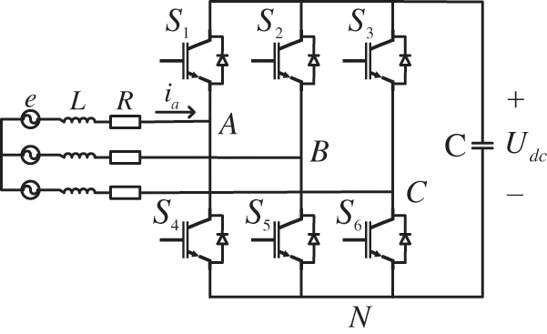
Figure 2: Simplified circuit diagram of voltage source PWM rectifier

Define the switching state as Eqs. (1)–(3):

Sa={1, if S1 on and S4 off0, if S1 off and S4 on(1)

Sb={1, if S2 on and S5 off0, if S2 off and S5 on(2)

Sc={1, if S3 on and S6 off0, if S3 off and S6 on(3)

Thus, the vectorial form of the switching state is defined as Eq. (4):

S=23(Sa+aSb+a2Sc)(4)

where a=ej2π3.

Define the PWM rectifier output voltage space vector as Eq. (5):

vαβ=23(vAN+avBN+a2vCN)(5)

where vAN,vBN, and vCN are the three-phase output phase-to-phase voltages of the PWM rectifier relative to the neutral point.

Then, the output voltage can be related to the switching state S as Eq. (6):

vαβ=VdcS(6)

where Vdc is the DC link voltage.

Analyzing all possible switching states, eight switching states can be obtained corresponding to eight voltage vectors. Because there are two switching states (000, 111) corresponding to the zero-voltage vector, there are 7 different voltage vectors. The voltage vector sector diagram is shown in Fig. 3.

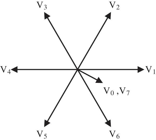
Figure 3: Voltage vector sector chart

Defining the PWM rectifier input current space vector as Eq. (7):

iαβ=23(ia+aib+a2ic)(7)

where ia,ib and ic are the three-phase input side currents of the PWM rectifier.

Simplify the circuit shown in Fig. 2 to obtain the circuit in the α−β coordinate system, as shown in Fig. 4.

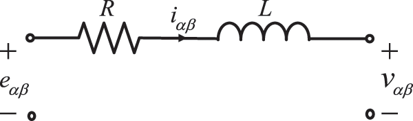
Figure 4: Equivalent circuit of α−β coordinate system

For the circuit shown in Fig. 4, Kirchhoff's law can be obtained by Eq. (8):

eαβ=iαβR+Ldiαβdt+vαβ(8)

where R is the equivalent resistance, L is the filter inductance, eαβ is the value of the power supply voltage in the α−β coordinate system, iαβ is the value of the input current in the α−β coordinate system, vαβ is the value of the rectifier output phase-to-phase voltage in the α−β coordinate system.

2.2.2 Discrete-Time Model

Since the FCS-MPC is an algorithm applied in discrete situations, it is necessary to establish a discrete-time mathematical model for analysis.

According to the Euler approximation formula, the discrete form of the current derivative formula based on the sampling time can be obtained by Eq. (9):

didt≈i(k)−i(k−1)Ts(9)

Replacing it in Eq. (8), the future load current can be obtained by Eq. (10):

i(k)=Li(k−1)+Tse(k)−Tsv(k)RTs+L(10)

Shifting the discrete-time one step forward in Eq. (10), the future load current can be determined as Eq. (11):

i(k+1)=Li(k)+Tse(k+1)−Tsv(k+1)RTs+L(11)

when the sampling period is small enough and the load is mainly inductive, RTs can be neglected and Eq. (11) can be expressed by Eq. (12):

i(k+1)=(1−RTsL)i(k)+TsL[e(k+1)−v(k+1)](12)

when the sampling frequency is much greater than the power supply frequency, it can be considered that the power-EMF does not change in one sampling interval so can assume as Eq. (13):

e(k+1)≈e(k)(13)

2.2.3 Load Simulation Side Control Strategy

After establishing the required discrete-time model, formulate a control scheme according to the required control objectives. Firstly, the analysis of the control strategy on the load simulation side is performed.

According to the needs of the power supply under test, set the load with the corresponded characteristics and calculate the reference input current iαβ∗(k). According to the Lagrange second-order extrapolation formula, the reference input current at the next moment can be expressed by Eq. (14):

iαβ∗(k+1)=3iαβ∗(k)−3iαβ∗(k−1)+iαβ∗(k−2)(14)

Set the cost function as Eq. (15):

g1=|iα∗(k+1)−iα(k+1)|+|iβ∗(k+1)−iβ(k+1)|(15)

Substitute all possible voltage vectors into Eq. (16):

i(k+1)=(1−RTsL)i(k)+TsL[e(k)−v(k)](16)

The obtained predicted current values at the next moment are compared through the cost function in turn. The switching state corresponding to the voltage vector that minimizes the cost function is taken as the switching signal at the next moment.

2.2.4 Energy Feedback Side Control Strategy

After determining the control strategy on the load simulation, formulate a control strategy to realize the control goals of the energy feedback side.

The control goals of the energy feedback side are to stabilize the DC bus voltage and control the phase angle and amplitude of the grid-connected side current to achieve unity power factor grid connection. In this paper, the PI controller is used to control the DC bus voltage. After that, the reference value of the active power is obtained. The current control on the grid-connected side is realized by setting the cost function.

According to the instantaneous power theory, the active power (p) and reactive power (q) of the circuit can be determined by Eq. (17):

{p=uαiα+uβiβq=uαiβ−uβiα(17)

where uα,uβ are the components of the three-phase voltage on the grid-connected side in the α−β coordinate system, iα,iβ are the components of the three-phase current on the grid-connected side in the α−β coordinate system.

The reference current at the next moment is still calculated by Eq. (14) whereas the predicted current at the next moment is obtained by Eq. (16).

Set the cost function as Eq. (18):

g2=|p∗(k+1)−p(k+1)|2+|q∗(k+1)−q(k+1)|2(18)

The reference current at the next moment used in the calculation of the active power reference value p∗(k+1) here is calculated by the PI controller. To achieve unity power factor grid connection, q∗(k+1) is set to 0 when considering the reactive power reference value.

2.2.5 Simplified Predictive Control Strategy

FCS-MPC does not have a strong universality in industrial applications because of its high computation burden and high computing power requirements of processors. To solve this problem, this paper adopts a simplified FCS-MPC, which greatly reduces the computational power of the algorithm, thus making it possible to implement the algorithm using low-cost processors. In this way, it can be adequately applied in future industries.

For the conventional FCS-MPC, the predicted current for the next moment is first calculated and then evaluated using a cost function. After that, the switching state corresponding to the voltage vector that minimizes the cost function is selected as the most possible switching state for the next moment. The conventional FCS-MPC block diagram is shown in Fig. 5.

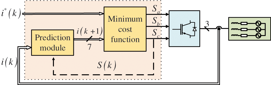
Figure 5: Conventional FCS-MPC control block diagram

It can be seen from Fig. 5 that the calculation process of the conventional FCS-MPC mainly includes predicting the current at the next moment and obtaining the minimum switching state through the cost function calculation and comparison.

Starting from the calculation process of the conventional FCS-MPC, it consists of two operations: prediction current (7 times) and evaluation of the cost function (7 times). The computational complexity of the algorithm can be reduced by simplifying the two parts of the calculation process.

The prediction current process is analyzed first. It is calculated based on the voltage vector corresponding to each switching state in turn to obtain all possible next-stage currents. Therefore, direct prediction of the voltage quantities can be considered and the reference voltage of the next stage is obtained from the reference current, followed by direct selection of the voltage vector using the cost function, as follows.

By replacing i(k+1) with i∗(k+1), Eq. (16) can be transformed as Eq. (19):

v∗(k+1)=e(k)−LTsi∗(k+1)+(LTs−R)i(k)(19)

The cost function becomes Eq. (20):

g3=|v∗(k+1)−v(k)|(20)

This simplifies the seven operations of the predicted current process to one.

Regarding the cost function evaluation process, the switching state corresponding to the current vector that makes the cost function take the minimum value is obtained by calculating and comparing each possible current vector according to the set cost function. Through the simplification of the predicted current process, the voltage vectors can be compared directly by calculation. However, the cost function evaluation process still requires seven judgments. The purpose of this process is to obtain the closest voltage vector. For this purpose, a sector allocation method like SVPWM can be considered for the voltage vector, dividing the area where the voltage vector is located into six sectors, and subsequently selecting the corresponding voltage vector by comparison calculations, thus, in this way, obtaining the most possible switching state for the next stage.

The simplified FCS-MPC voltage vector sector distribution diagram is shown in Fig. 6. According to the vector operation, the point with the same displacement from the origin and the endpoints of the six voltage vectors is found and the boundary of the shaded region in Fig. 6 can be obtained. Based on geometric knowledge, it is known that the boundary of the shaded area is the vertical bisector corresponding to the voltage vectors V1~V6, and the points on the vertical bisector have equal distances to the two endpoints. Then it can be derived that the voltage vector in the shaded region is closer to the zero vector (V0, V7), and the voltage vector outside the shaded region is closer to the corresponding switching voltage vector (V1~V6) in that region.

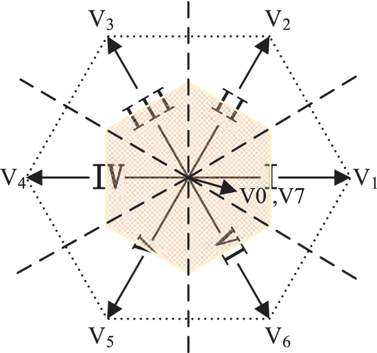
Figure 6: Simplified FCS-MPC voltage vector sector diagram

The specific steps to simplify the FCS-MPC are as follows:

1) Calculate v∗(k+1) from equation Eq. (17);

2) Determine the sector where v∗(k+1) in which the SVPWM is located by the sector determination method;

3) Judge whether v∗(k+1) is in the shaded area and select the switch state corresponding to the zero vector if it is in the shaded area, or select the switch state corresponding to the voltage vector in that sector if it is not in the shaded area.

The simplified FCS-MPC block diagram is shown in Fig. 7. It can be seen from Fig. 7 that the simplified FCS-MPC no longer requires complex current calculation and cost function calculation. After converting it into voltage calculation and sector distribution, the computational complexity is effectively reduced.

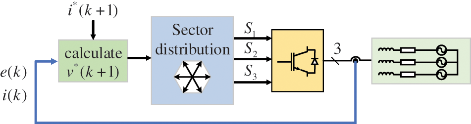
Figure 7: Simplified FCS-MPC control block diagram

2.2.6 System Control Strategy

The system operates under symmetrical three-phase conditions. The overall block diagram of the control system is shown in Figs. 8 and 9.

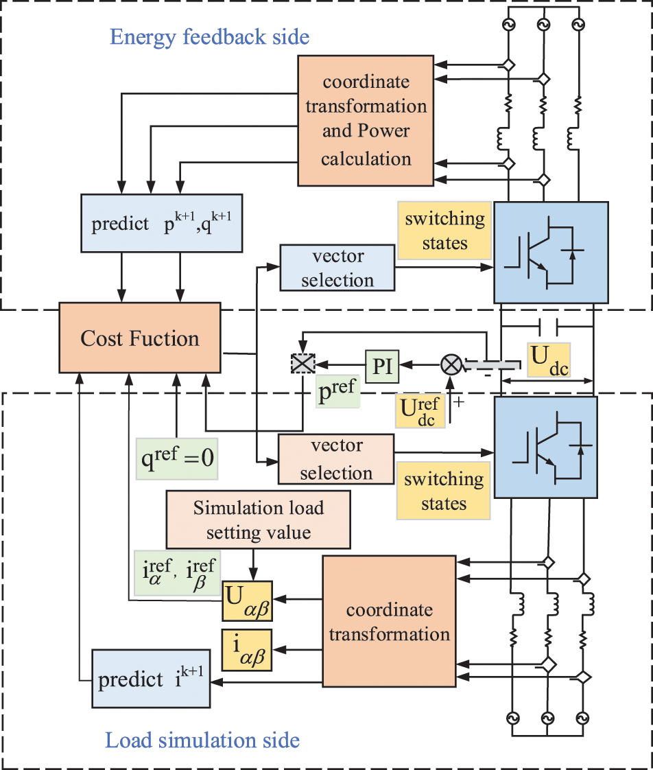
Figure 8: System control block diagram (Conventional FCS-MPC)

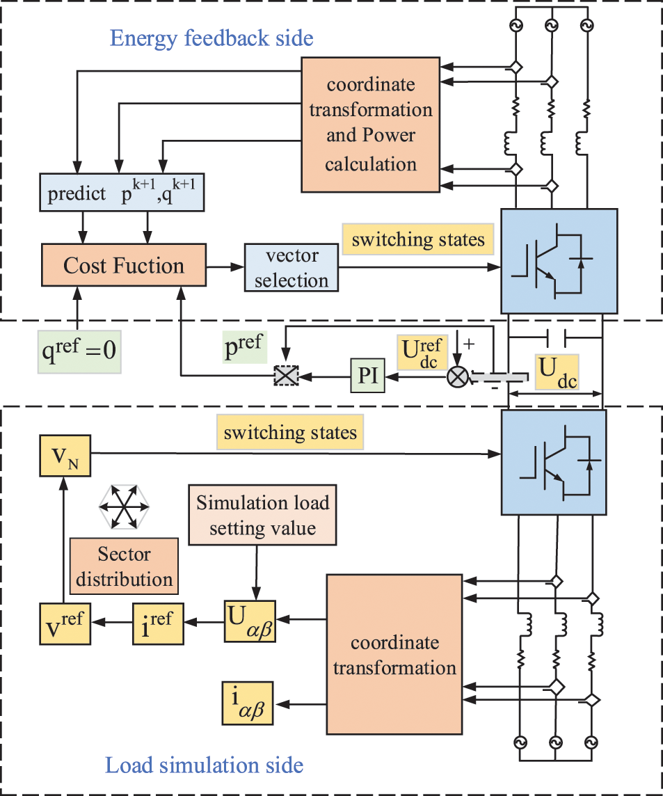
Figure 9: System control block diagram (Simplified FCS-MPC)

In Fig. 8, for conventional FCS-MPC, the control on the load simulation side adopts direct predictive current control. After calculating the reference current and all possible currents at the next moment and setting the cost function, the switching state of the next stage is obtained.

In Fig. 9, for simplified FCS-MPC, the control on the load simulation side avoids the complex calculation process of conventional FCS-MPC. By calculating the reference voltage corresponding to the reference current, and then judging the voltage vector with the smallest difference with the reference voltage vector, the switching state of the next stage is obtained.

2.2.7 System Stability Analysis

The system stability analysis of FCS-MPC. Since FCS-MPC has no specific transfer function, its stability analysis can only be done through simplified analysis.

In [27], the author presented a method to obtain the transfer function of FCS-MPC. Since the focus of the AC electronic load is to control the current on the input side, this paper only briefly analyzes the current control loop of the front stage. The simplified block diagram is shown as Fig. 10.

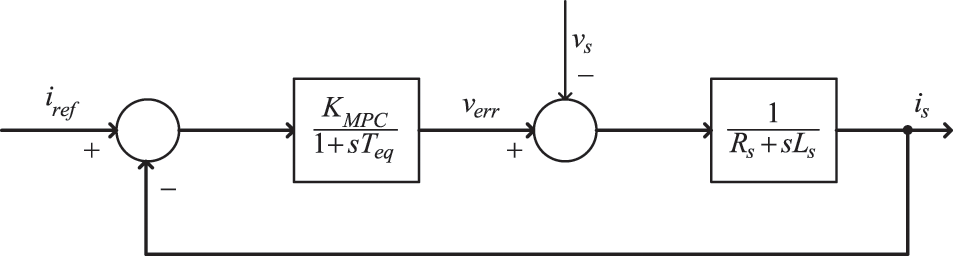
Figure 10: Simplified block diagram of input current control loop

In Fig. 10, verr is the difference between the reference and predicted value of the rectifier voltage, Teq is the equivalent time constant, assume the statistical execution delay of the MPC controller is 0.1Ts, where Ts is 50 μs. Considering the A/D conversion delay is 0.05 Ts, so the Teq can be calculated as Eq. (21):

Teq=0.85Ts(21)

The transfer function of the current control loop can be transformed as Eq. (22):

Gi(s)=KMPCs2TeqL+s(RTeq+L)+(R+KMPC)(22)

where KMPC is the constant gain of the FCS-MPC.

The Root locus diagram and the Nyquist diagram of the current control loop are shown as Figs. 11 and 12. The analysis results of the two analysis methods ensure the stability of the system.

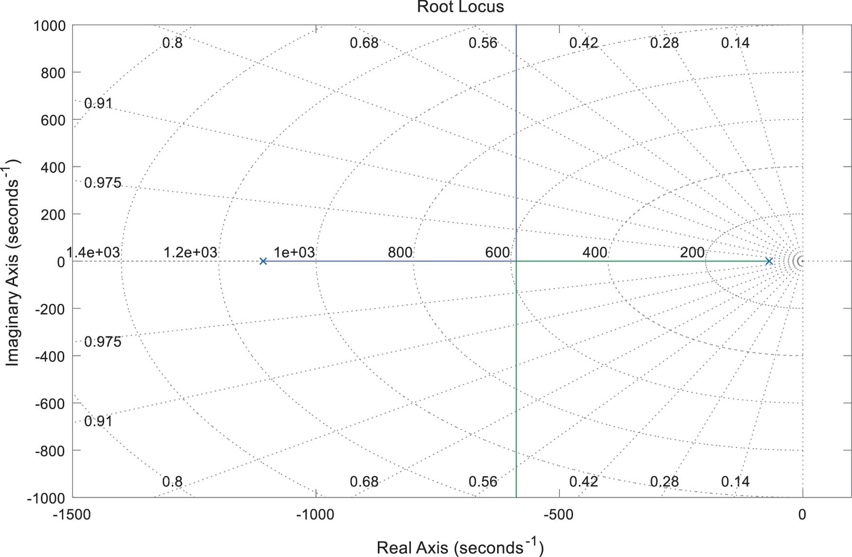
Figure 11: Root locus diagram for the transfer function of current control loop

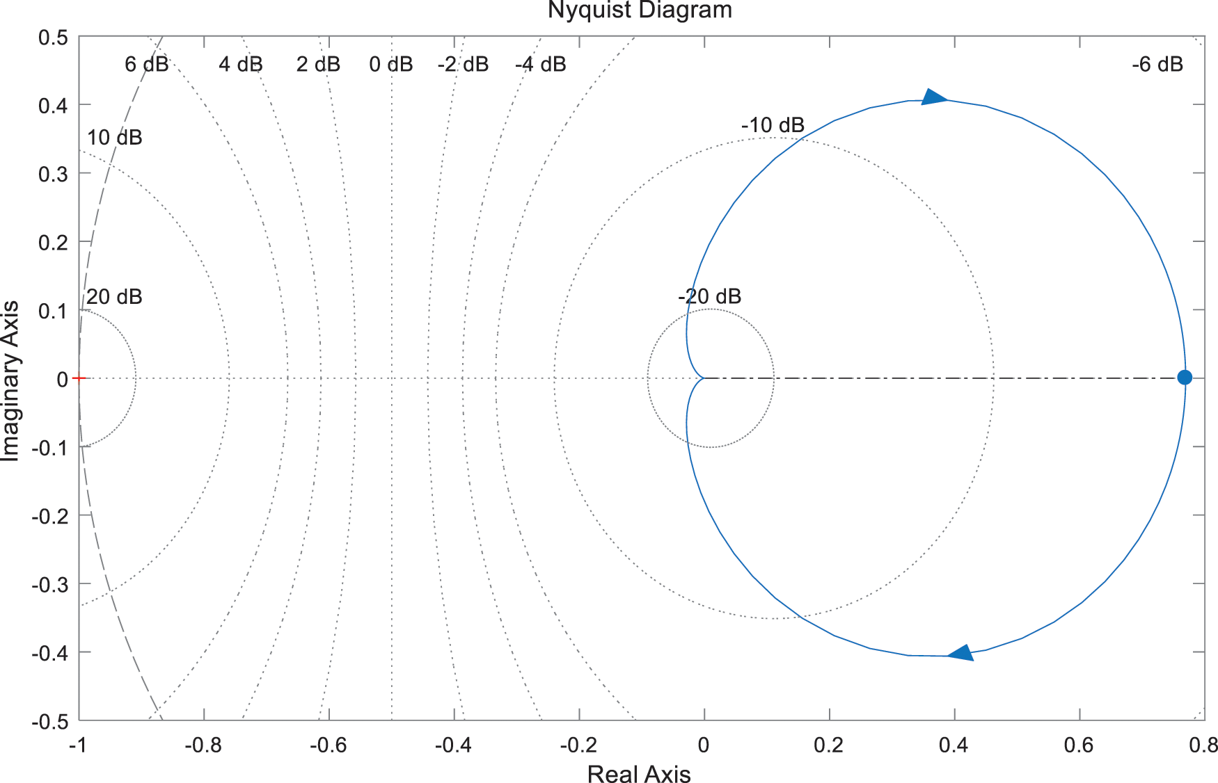
Figure 12: Nyquist diagram for the transfer function of current control loop

3  Simulation Results

The simulation consists of two parts. The first part is to compare the control performance of simplified FCS-MPC with SVPWM and FCS-MPC. The second part is to observe the control performance of the simplified FCS-MPC on the AC electronic load with energy recovery.

The AC electronic load with energy recovery controlled by SVPWM, FCS-MPC and simplified FCS-MPC are simulated by MATLAB/Simulink. The simulation parameters are shown in Table 1.

3.1 Performance Comparison

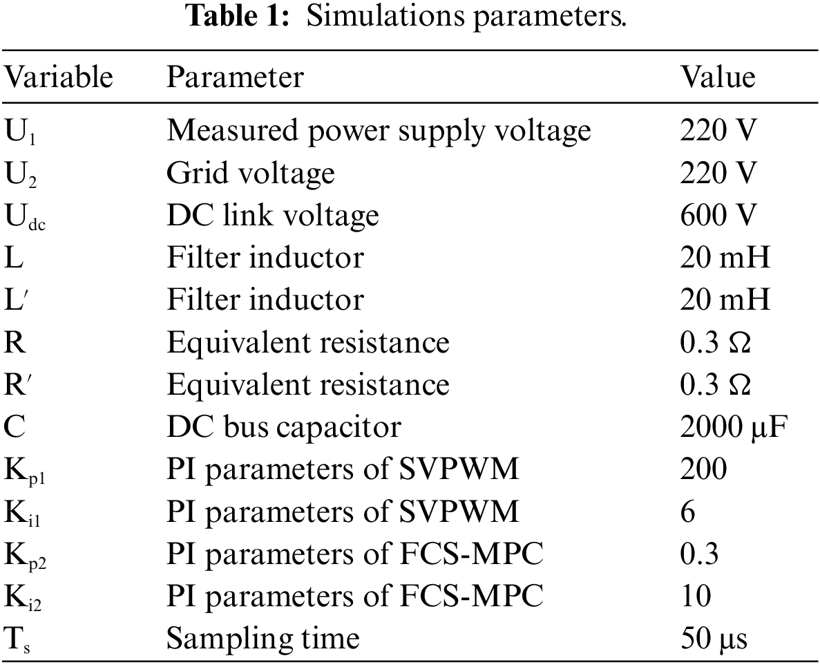
Taking the simulated pure resistive load as an example, the simulated reference current is set to15 A. The current tracking effect of iα and iβ under the control of SVPWM and FCS-MPC is shown in Fig. 13.

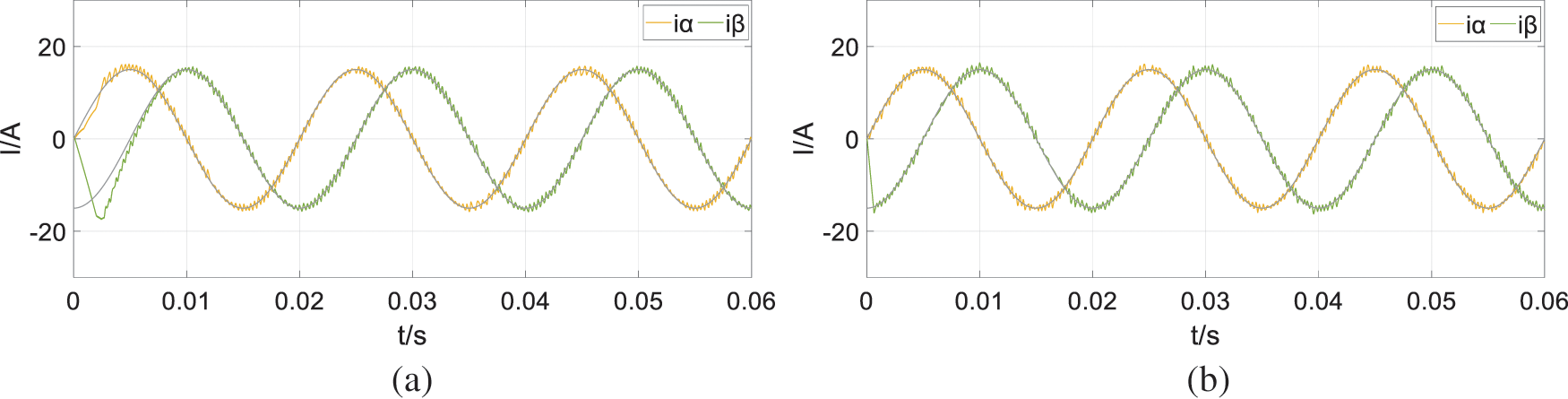
Figure 13: Simulation results when the load simulation side current is 15 A (a) SVPWM (b) FCS-MPC

It is demonstrated that with the same post-stage control, the load simulation side with FCS-MPC control has better rapidity. FCS-MPC can reach steady state almost instantaneously, while SVPWM takes nearly 0.005 s to reach steady state. It also reaches the steady state smoother and has comparable steady-state performance with SVPWM. The current tracking effect is very close as well.

The current is set to change abruptly, and the amplitude is reduced from 15 to 10 A at t = 0.015 s to observe the control effect of the two algorithms, the simulation results are shown in Fig. 14. From the simulation results, it can be seen that the FCS-MPC can return to the steady state faster and smoother when the current changes abruptly, which indicates that the FCS-MPC has better dynamic response performance than the SVPWM.

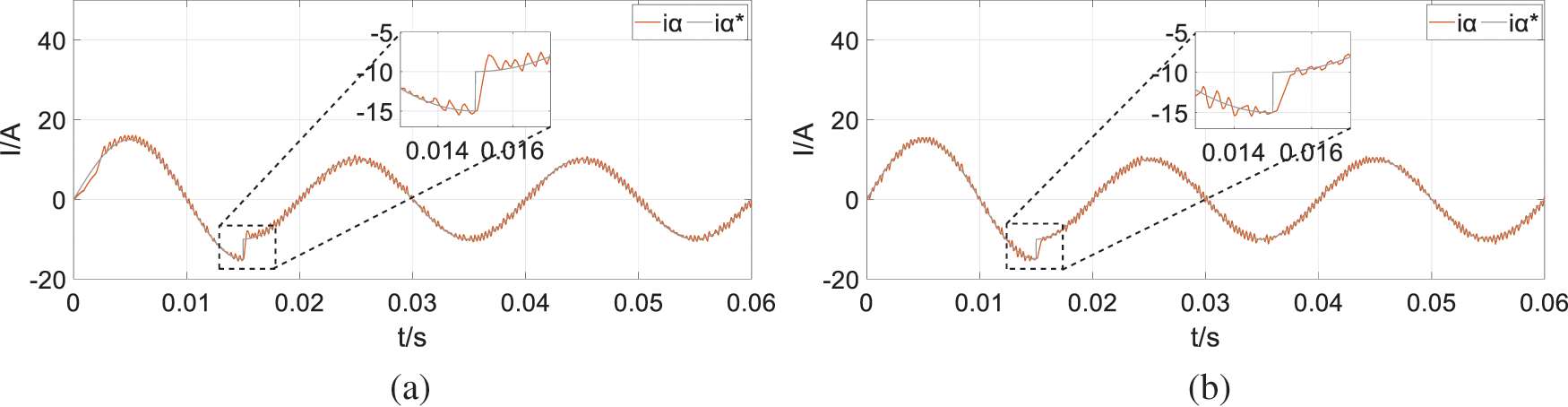
Figure 14: Simulation results when the load simulation side current change (a) SVPWM (b) FCS-MPC

Due to the large amount of calculation of FCS-MPC, some delay problems may occur which could lead to poor tracking effect. A relatively simple and effective delay compensation scheme is proposed in [28] to improve the steady-state behavior of FCS-MPC. This research increases the switching frequency to improve the control performance of FCS-MPC. When the sampling time is set to20 μs, the simulation result is shown in Fig. 15.

Figure 15: Experimental result with Ts = 20 μs for a step on iα∗

The simulation results show that the steady-state performance and transient performance of FCS-MPC have been improved after using a smaller sampling time. Therefore, we believe that FCS-MPC is a satisfying control algorithm with good high frequency performance.

In Fig. 13, the current on the load simulation side under SVPWM control has an obvious transient transition process at the beginning. The transient time is too long compared with the predictive control. In order to meet the current demand for high-power electronic load simulation, the ability of the control algorithm to track large currents is particularly important. We increase the load reference current amplitude to 25 A and observe the tracking effect of the two algorithms. The simulation results are shown in Fig. 16.

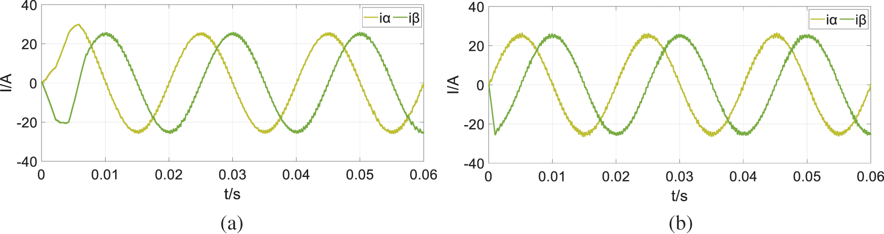
Figure 16: Simulation results when the load simulation side current is 25 A (a) SVPWM (b) FCS-MPC

It is clearly illustrated that after the current amplitude increases, the initial transient time of the load simulation side current controlled by the SVPWM algorithm becomes longer, increase to about 0.075 s, which is not benefit for the control of AC electronic loads that require fast response. On the contrary, after the current amplitude of the FCS-MPC algorithm increases, the transient process does not change significantly. The current tracking effect is improved to a certain extent instead. Therefore, it can be concluded that FCS-MPC is a control algorithm that is more suitable for simulating high-power loads.

Through FFT analysis, the THD results of FCS-MPC when the simulated load current has different amplitudes are obtained as shown in Table 2. It is not difficult to see that when the simulated load current is larger, the input current of the load simulation side has a lower THD, which has a better effect on the high-power load simulation test of the AC power supply.

The simplified FCS-MPC is simulated and analyzed. The simulated reference current is set to15 A and its performance is observed in Figs. 17 and 18.

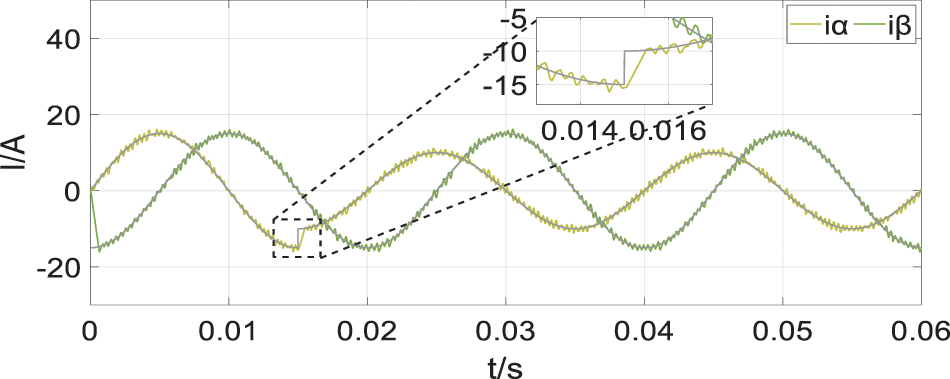
Figure 17: Simulation results for simplified FCS-MPC

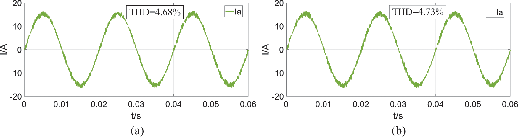
Figure 18: The waveform and THD of load simulation side current Ia (a) FCS-MPC (b) simplified FCS-MPC

The DC link voltage changes in both methods are shown in Fig. 19.

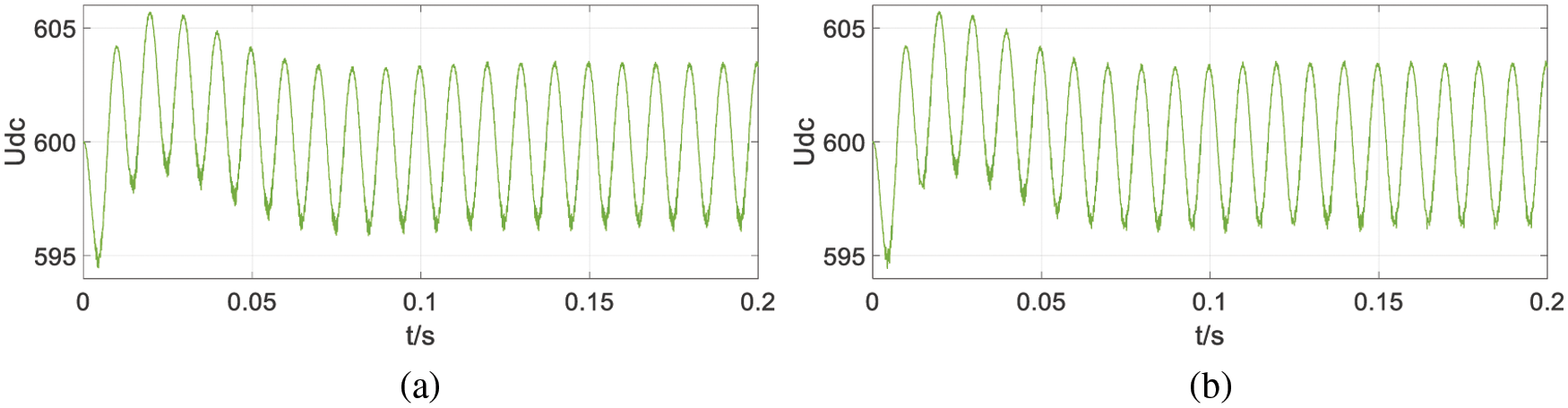
Figure 19: The DC link voltage (a) FCS-MPC (b) simplified FCS-MPC

It can be seen from the simulation results that its steady-state performance and transient performance are very similar to those of traditional FCS-MPC. The DC bus voltage changes of the two methods are also almost constant. The algorithms mentioned in this article are implemented using the S-Function module in SIMULINK. Using the MATLAB function running time analysis (Profile Function), the running time of each module corresponding to FCS-MPC and the simplified FCS-MPC algorithm under the same simulation time is shown in Fig. 20.

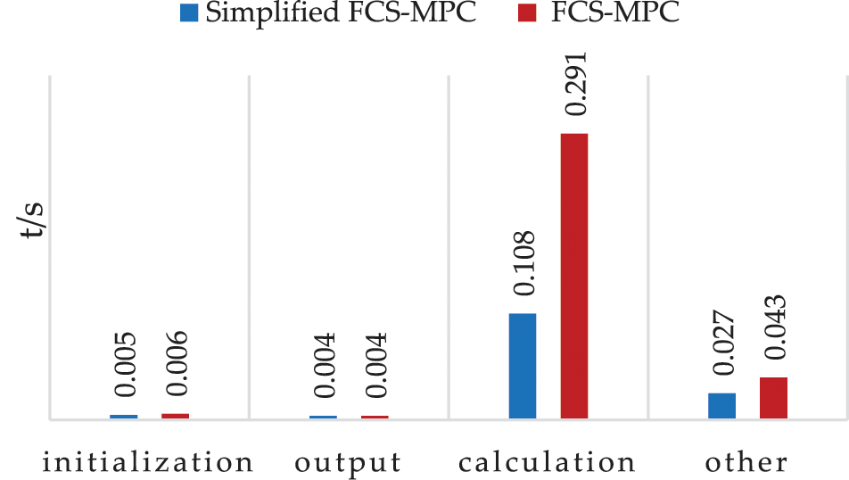
Figure 20: The running time of each module of the algorithm

The time spent by the calculation module of the corresponding prediction algorithm in the S-Function of FCS-MPC is about three times that of the simplified FCS-MPC while the total time is about twice that of the simplified FCS-MPC. This shows that the simplified FCS-MPC can greatly reduce the calculation amount. The computation burden of the processor is effectively reduced. It allows lower performance requirements of the processor, which greatly increases the ubiquity of FCS-MPC applications. To sum up, simplifying the FCS-MPC algorithm is a benefit improvement.

Analyze the robustness of the system. Considering the model mismatch problem of FCS-MPC, the system control effect in the case of model mismatch is shown in Figs. 21 and 22.

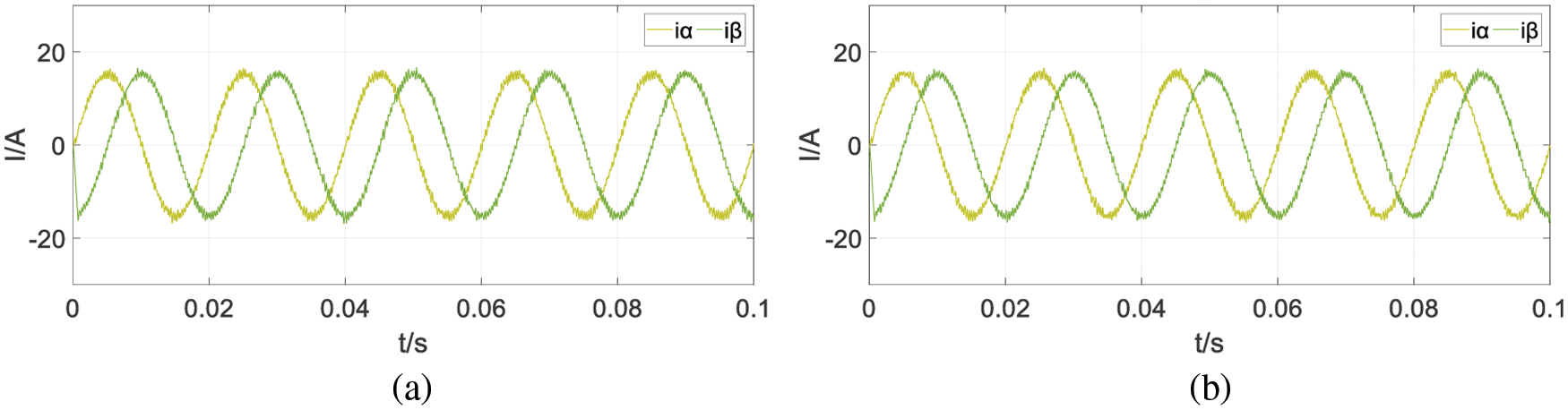
Figure 21: The simulation results in (a) R/R0 = 0.5 (b) R/R0 = 2

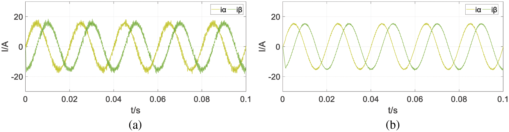
Figure 22: The simulation results in (a) L/L0 = 0.5 (b) L/L0 = 2

It can be seen from the simulation results that the change of the load resistance has no obvious effect on the simulation results of the system, but the change of the load inductance has a great influence on the steady-state error of the system. When the load inductance is less than the standard value, it will increase the system’s steady-state error.

3.2 System Control Performance

In order to further observe the control performance of the simplified FCS-MPC on the AC electronic load with energy recovery, the inductive load and the capacitive load are simulated respectively to observe the control results.

The simulation results of the inductive load Z1 = 6 + j6 (impedance angle of 45°) and capacitive load Z2 = 6 − j6 (impedance angle of −45°) are shown in Figs. 23 and 24. From simulation results, it can be seen that the simplified FCS-MPC can be well simulate these two types of loads, the waveform shows very good current tracking effect.

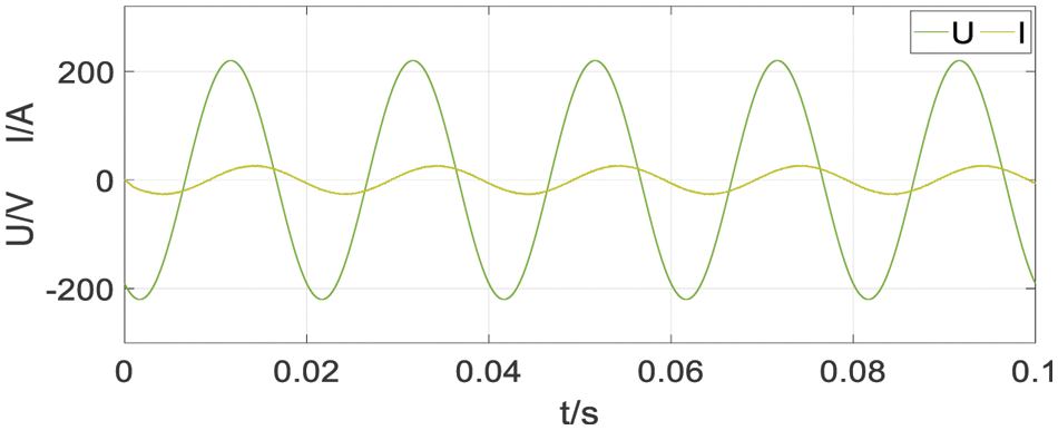
Figure 23: Simulation result of inductive load

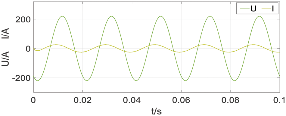
Figure 24: Simulation result of capacitive load

In Fig. 25, the simulation result of time-varying load is shown. It is obvious that the proposed control system can operate under time-varying loads.

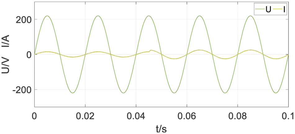
Figure 25: Simulation result of time-varying load (t = 0.045 s, I from 15 to 25 A)

Under the rear stage control, the energy feedback side needs to achieve the control goal of unity power factor grid connection. FFT analysis of the three-phase current on the grid-connected side when simulating Z1. The simulation results are shown in Figs. 26 and 27. A unity power factor grid connection is achieved with a lower THD, compliant with industry standards.

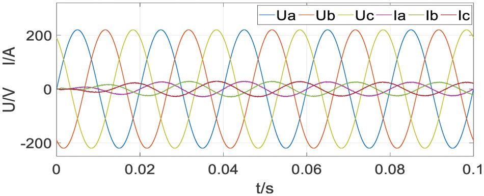
Figure 26: Three-phase voltage and current of the energy feedback side

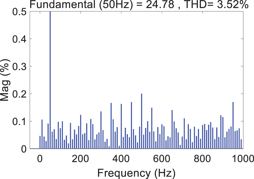
Figure 27: FFT analysis result of the grid side current

4  Conclusions

In this paper, the feasibility of FCS-MPC in controlling AC electronic load with energy recovery is verified through simulation verification, followed by analysis on its good performance when simulating high-power loads. After that a simplified FCS-MPC through sector judgment is proposed. The computational complexity of the algorithm is greatly reduced, the number of calculations has been reduced from 14 times to only one calculation and one sector judgment, it can be implemented with low-cost processors, making it more realistic to put it into practical applications. The stability and robustness of the algorithm are proved by the equivalent transformation analysis. Compared with the SVPWM algorithm, it is confirmed that FCS-MPC has better dynamic performance and anti-interference. In normal simulation, it generally reaches steady state 0.005 s earlier than SVPWM. It also shows good simulation results for loads with different characteristics. It can be concluded that simplified FCS-MPC is a better alternative algorithm for AC electronic load with energy recovery, providing a new alternative for engineering practice applications.

Funding Statement: The authors received no specific funding for this study.

Conflicts of Interest: The authors declare that they have no conflicts of interest to report regarding the present study.

References

    1. Zhang, Z., Liu, X., Zhang, Y., Zhang, C., Deng, W. (2021). A novel current control method based on dual-mode structure repetitive control for three-phase power electronic load. IEEE Access, 9, 144406–144416. DOI 10.1109/ACCESS.2021.3122123. [Google Scholar] [CrossRef]

    2. Akhlaghi, S., Zolghadri, M. (2020). Predictive current control for programmable electronic AC load. 2020 11th Power Electronics, Drive Systems, and Technologies Conference (PEDSTC), pp. 1–5. Tehran, Iran. DOI 10.1109/PEDSTC49159.2020.9088471. [Google Scholar] [CrossRef]

    3. Benjanarasut, K., Benjanarasut, J., Neammanee, B. (2017). Single phase AC electronic load with energy recovery. 2017 International Electrical Engineering Congress (iEECON), pp. 1–4. Pattaya, Thailand. DOI 10.1109/IEECON.2017.8075777. [Google Scholar] [CrossRef]

    4. Geng, Z., Gu, D., Hong, T., Czarkowski, D. (2018). Programmable electronic AC load based on a hybrid multilevel voltage source inverter. IEEE Transactions on Industry Applications, 54(5), 5512–5522. DOI 10.1109/TIA.2018.2818059. [Google Scholar] [CrossRef]

    5. Li, F., Zou, Y. P., Wang, C. Z., Chen, W., Zhang, Y. C. et al. (2008). Research on AC electronic load based on back to back single-phase PWM rectifiers. 2008 Twenty-Third Annual IEEE Applied Power Electronics Conference and Exposition, pp. 630–634. Austin, TX, USA. DOI 10.1109/APEC.2008.4522787. [Google Scholar] [CrossRef]

    6. Ji, T. C., Qi, Y. C., Zhao, H. T. (2020). Research on control strategy of new current-type energy-fed AC electronic load. 2020 IEEE Sustainable Power and Energy Conference (iSPEC), pp. 258–263. Chengdu, China. DOI 10.1109/iSPEC50848.2020.9351144. [Google Scholar] [CrossRef]

    7. Chavali, R. V., Dey, A., Das, B. (2022). A hysteresis current controller PWM scheme applied to three-level NPC inverter for distributed generation interface. IEEE Transactions on Power Electronics, 37(2), 1486–1495. DOI 10.1109/TPEL.2021.3107618. [Google Scholar] [CrossRef]

    8. Wang, S., Ma, J., Liu, B., Jiao, N., Liu, T. et al. (2020). Unified SVPWM algorithm and optimization for single-phase three-level NPC converters. IEEE Transactions on Power Electronics, 35(7), 7702–7712. DOI 10.1109/TPEL.2019.2960208. [Google Scholar] [CrossRef]

    9. Cortes, P., Kazmierkowski, M. P., Kennel, R. M., Quevedo, D. E., Rodriguez, J. (2008). Predictive control in power electronics and drives. IEEE Transactions on Industrial Electronics, 55(12), 4312–4324. DOI 10.1109/TIE.2008.2007480. [Google Scholar] [CrossRef]

  10. Kouro, S., Cortes, P., Vargas, R., Ammann, U., Rodriguez, J. (2009). Model predictive control—A simple and powerful method to control power converters. IEEE Transactions on Industrial Electronics, 56(6), 1826–1838. DOI 10.1109/TIE.2008.2008349. [Google Scholar] [CrossRef]

  11. Rodriguez, J., Kazmierkowski, M. P., Espinoza, J. R., Zanchetta, P., Abu-Rub, H. et al. (2013). State of the art of finite control set model predictive control in power electronics. IEEE Transactions on Industrial Informatics, 9(2), 1003–1016. DOI 10.1109/TII.2012.2221469. [Google Scholar] [CrossRef]

  12. Karamanakos, P., Geyer, T. (2020). Guidelines for the design of finite control set model predictive controllers. IEEE Transactions on Power Electronics, 35(7), 7434–7450. DOI 10.1109/TPEL.2019.2954357. [Google Scholar] [CrossRef]

  13. Gulbudak, O., Santi, E. (2016). Finite control set model predictive control of dual-output four-leg indirect matrix converter under unbalanced load and supply conditions. 2016 IEEE Applied Power Electronics Conference and Exposition (APEC), Long Beach, CA, USA. DOI 10.1109/apec.2016.7468331. [Google Scholar] [CrossRef]

  14. Gulbudak, O., Santi, E., Marquart, J. (2014). Finite state model predictive control for 3×3 matrix converter based on switching state elimination. 2014 IEEE Energy Conversion Congress and Exposition (ECCE), Pittsburgh, PA, USA. DOI 10.1109/ecce.2014.6954198. [Google Scholar] [CrossRef]

  15. Gulbudak, O., Gokdag, M., Komurcugil, H. (2022). Model predictive control strategy for induction motor drive using Lyapunov stability objective. IEEE Transactions on Industrial Electronics, 69(12), 12119–12128. DOI 10.1109/TIE.2021.3139237. [Google Scholar] [CrossRef]

  16. Babaie, M., Mehrasa, M., Sharifzadeh, M., Al-Haddad, K. (2022). Floating weighting factors ANN-MPC based on Lyapunov stability for seven-level modified PUC active rectifier. IEEE Transactions on Industrial Electronics, 69(1), 387–398. DOI 10.1109/TIE.2021.3050375. [Google Scholar] [CrossRef]

  17. Babaie, M., Mehrasa, M., Sharifzadeh, M., Al-Haddad, K. (2021). Floating weighting factors ANN-MPC based on Lyapunov stability for seven-level modified PUC active rectifier. IEEE Transactions on Industrial Electronics, 69(1), 387–398. DOI 10.1109/TIE.2021.3050375. [Google Scholar] [CrossRef]

  18. Wang, F., Lin, G., He, Y. (2021). Passivity-based model predictive control of three-level inverter-fed induction motor. IEEE Transactions on Power Electronics, 36(2), 1984–1993. DOI 10.1109/TPEL.2020.3008915. [Google Scholar] [CrossRef]

  19. Vazquez, S., Rodriguez, J., Rivera, M., Franquelo, L. G., Norambuena, M. (2017). Model predictive control for power converters and drives: Advances and trends. IEEE Transactions on Industrial Electronics, 64(2), 935–947. DOI 10.1109/TIE.2016.2625238. [Google Scholar] [CrossRef]

  20. Kwak, S., Park, J. (2014). Switching strategy based on model predictive control of VSI to obtain high efficiency and balanced loss distribution. IEEE Transactions on Power Electronics, 29(9), 4551–4567. DOI 10.1109/TPEL.2013.2286407. [Google Scholar] [CrossRef]

  21. Geyer, T., Quevedo, D. E. (2015). Performance of multistep finite control set model predictive control for power electronics. IEEE Transactions on Power Electronics, 30(3), 1633–1644. DOI 10.1109/TPEL.2014.2316173. [Google Scholar] [CrossRef]

  22. Harbi, I., Abdelrahem, M., Ahmed, M., Kennel, R. (2020). Reduced-complexity model predictive control with online parameter assessment for a grid-connected single-phase multilevel inverter. Sustainability, 12(19), 7997. DOI 10.3390/su12197997. [Google Scholar] [CrossRef]

  23. Kieferndorf, F., Karamanakos, P., Bader, P., Oikonomou, N., Geyer, T. (2012). Model predictive control of the internal voltages of a five-level active neutral point clamped converter. 2012 IEEE Energy Conversion Congress and Exposition (ECCE), pp. 1676–1683. Raleigh, NC, USA. DOI 10.1109/ECCE.2012.6342611. [Google Scholar] [CrossRef]

  24. Yin, J., Leon, J. I., Perez, M. A., Franquelo, L. G., Marquez, A. et al. (2021). Model predictive control of modular multilevel converters using quadratic programming. IEEE Transactions on Power Electronics, 36(6), 7012–7025. DOI 10.1109/TPEL.2020.3034294. [Google Scholar] [CrossRef]

  25. Gao, J., Gong, C., Li, W., Liu, J. (2020). Novel compensation strategy for calculation delay of finite control set model predictive current control in PMSM. IEEE Transactions on Industrial Electronics, 67(7), 5816–5819. DOI 10.1109/tie.2019.2934060. [Google Scholar] [CrossRef]

  26. Serna-Montoya, L. F., Cano-Quintero, J. B., Muñoz-Galeano, N., López-Lezama, J. M. (2019). Programmable electronic AC loads: A review on hardware topologies. 2019 IEEE Workshop on Power Electronics and Power Quality Applications (PEPQA), pp. 1–6. Manizales, Colombia. DOI 10.1109/PEPQA.2019.8851542. [Google Scholar] [CrossRef]

  27. Parvez, M., Mekhilef, S., Tan, N. M. L., Akagi, H. (2015). An improved active-front-end rectifier using model predictive control. 2015 IEEE Applied Power Electronics Conference and Exposition(APEC), Charlotte, NC, USA. DOI 10.1109/apec.2015.7104341. [Google Scholar] [CrossRef]

  28. Cortes, P., Rodriguez, J., Silva, C., Flores, A. (2012). Delay compensation in model predictive current control of a three-phase inverter. IEEE Transactions on Industrial Electronics, 59(2), 1323–1325. DOI 10.1109/TIE.2011.2157284. [Google Scholar] [CrossRef]