Cayley Picture Fuzzy Graphs and Interconnected Networks

1  Introduction

A classical (crisp) set involves exactly two truth values ‘True (1)’ and ‘False (0)’ which is unable to handle the raw data or the data with uncertainties. To overcome such circumstances, Zadeh [1] explored the concepts of fuzzy sets (FSs) which is proved more effective to solve the problems containing uncertainties. The fuzzy sets (FSs) is the generalized form of a classical (crisp) set in which the members of the set are allocated different degrees of membership values lying in the interval [0,1] . Since allotting a fixed number to the judgement of any specialist in any field of life becomes very constrictive, so it would be more effective if we take an interval rather than a specific number. Hence the term interval-valued fuzzy sets (IVFSs) was proposed in [2]. Further to this, by introducing an additional membership degree named “hesitation margin” in the fuzzy sets the term intuitionistic fuzzy sets (IFSs) was introduced in [3]. IFSs is comparatively more efficient than the typical fuzzy sets to handle uncertainty because it has an extra margin i.e., “hesitation margin”. Moreover, IFSs was applied effectively in different fields of sciences like image processing [4], decision making [5] etc. However, it has been observed that in IFS the concept of the degree of neutrality cannot be considered. But neutrality degree has much importance in many real life circumstances like democratic election stations and so forth. Human beings normally give their judgments including more replies of the types: yes, no, abstain and refusal. In such types of situations, if we apply intuitionistic fuzzy sets theory then the details of voting for non-candidates (refusal) may be not considered. For handling such types of situations, Cuong [6] commenced with the idea of the picture fuzzy sets (PFSs) which is the generalized form IFSs. Picture fuzzy set (PFS) includes the concept of positive membership, neutral membership and negative membership degrees of each object. Subsequently, Phong et al. [7] proposed numerous picture fuzzy relations, Cuong and Hai [8] discussed several new types of operators in the setting of PFSs. Similarly, Garg [9] endorsed some aggregation operations of PFSs and explored its applications towards multi-criteria decision making. Furthermore, the generalization of picture fuzzy sets termed interval-valued picture fuzzy sets (IVPFSs) was introduced in [10]. Applications of interval-valued picture fuzzy soft sets (IVPFSs) towards decision-making theory were also explored by Khalil et al. [10].

The idea of fuzzy graphs (FGs) was proposed by Rosenfeld [11], a decade after the Zadeh’s incredible article on fuzzy sets. Fuzzy graphs are proven an effective tool to handle the problems containing unclear data. Fuzzy graph also provides us more compatible models for the solution of real world problems as compared to the classic graphs. Subsequently, Mordeson and Nair [12] introduced the concept of the complement fuzzy graph and in continuation Sunitha and Kumar explored it further in [13]. In the same perspective, Parvathi et al. [14] introduced the term intuitionistic fuzzy graphs (IFGs) at the base of intuitionistic fuzzy relation and Shannon and Atanossov [15] provided several generalized forms of IFGs. Different operations on IFGs were presented in [16,17]. Moreover, Rashmanlou et al. [18] discussed various exclusive properties of IFGs and different types of products of IFGs were discussed in [19]. The structure of IFGs has more diversity than that of FGs and hence several applications of IFGs were explored towards radio coverage networking [20], shortest path problems [21] and social networks [22]. Moreover, the term Cayley intuitionistic fuzzy graphs were discussed in [23]. Currently, the generalization of intuitionistic fuzzy graphs termed picture fuzzy graphs (PFGs) is introduced by Zua et al. [24]. They introduced some special types of picture fuzzy graphs (PFGs) like strong, complete etc. They also introduced and applied the terms weak and co-weak isomorphisms to the picture fuzzy graphs (PFGs). Few applications of PFGs towards social networking were also explored by them. Subsequently, picture fuzzy multigraphs (PFMGs) has been introduced in literature [25]. Recently, the further extensions of PFGs like constant picture fuzzy graphs [26] and balanced picture fuzzy graphs [27] are also introduced. First and third authors (with Babir Ali) have introduced the notion of bipolar picture fuzzy graphs and bipolar picture fuzzy acquaintanceship graph in [28]. Similarly, the term interval-valued picture fuzzy graphs is explored by both the authors in [29].

Numerous generalizations of the fuzzy graphs are explored in the literature to deal with the uncertainties existing in daily life complex problems. We know that the uncertainties are well explained by using PFSs and hence the Cayley picture fuzzy graphs (CPFGs) would be the excellent research area for dealing the problems having uncertainties. In this study, we suggest the definition of CPFGs at the base of picture fuzzy relation described on the group and its generators. We discuss few main characteristics of the Cayley picture fuzzy graphs. We show that the CPFGs are vertex transitive (node symmetric) and hence are regular. Consequently, we provide the linkage between Cayley picture fuzzy graphs and classical Cayley graphs as well. We discuss in detail the term connectivity of the CPFGs. Overall, we provide the generalizations of some characteristics of both the PFGs and Cayley fuzzy graphs (CFGs) in the setting of CPFGs. Finally, we provide an application of CPFGs towards interconnected networks.

2  Preliminaries

Definition 1. [1] A pair (Υ,X) , where X is a nonempty set and Υ:X→[0,1] is the membership function, is said to be a fuzzy set (subset) (FS) of X .

Definition 2. [1] A fuzzy subset of X×X is the fuzzy relation on any set X .

Definition 3. [30] An object of the form of S={(u,PS(u),QS(u):u∈U)} , where PS(u)∈[0,1] is the membership degree, QS(u)∈[0,1] is the non-membership degree of u , and PS and QS satisfy PS(u)+QS(u)≤1 , for all u∈U , is an intuitionistic fuzzy set (IFS) on U .

Definition 4. [6] A picture fuzzy set (PFS) S on a nonempty set U is the object expressible in the form of S= {(u,PS(u),QS(u),RS(u)):u∈U} , where Ps(u)∈[0,1] is the degree of positive membership, QS(u)∈[0,1] is the neutral membership degree while RS(u)∈[0,1] is the negative membership degree of u in S , and PS,QS and RS satisfy PS(u)+QS(u)+RS(u)≤1 , for all u∈X . Here, the refusal membership degree of u in S is 1−(PS(u)+QS(u)+RS(u).

Definition 5. [6] Let S={(u,PS(u),QS(u),RS(u)):u∈U} and T={(v,PT(v),QT(v),RT(v)) :v∈V} be two PFSs defined on U and V , respectively. Then their Cartesian product is given by

(i)S×1T={(u,v),PS(u).PT(v),QS(u).QB(v),RS(u).RS(v):u∈U,v∈V}

(ii)S×2T={(u,v),PS(u)∧PT(v),QS(u)∧QT(v),RS(u)∨RT(v):u∈U,v∈V}.

Definition 6. [11] Let V≠0 and finite set of vertices. Then G = (PC,PD) is a fuzzy graph, where PC is a fuzzy subset of V and PD is a symmetric fuzzy relation on PC, i.e., PC : V→ [0,1] and PD : V×V → [0,1] satisfying

PD(u,v)≤PC(u)∧PC(v),∀u,∀v∈V.

Definition 7. [23] Cayley intuitionistic fuzzy graph G=(V,R) of the graph is an IFG with the set of nodes or vertices V=G (a group) and let V=(ξ,ω) be an intuitionistic fuzzy subset of V and also R is an intuitionistic fuzzy subset on V×V is defined by

R(a,b)={(ξ(a−1b),ψ(a−1b)): a,b∈G  and  a−1b∈T⊆G}.

Definition 8. [24] A pair G=(C,D) is said to be a PFG on a H∗ = (A,B) , where C = (ηC,θC,ϑC) is a PFS on A and D = (ηD,θD,ϑD) is a PFS over the set B ⊆ A×A such that for any edge mn∈B with

ηD(m,n)≤min(ηC(m),ηC(n))

θD(m,n)≤min(θC(m),θC(n))

ϑD(m,n)≥max(ϑC(m),ϑC(n)).

Let G = (ξ, Υ) be a FG. The strength of connectedness between the pair of vertices u and v is the maximum of strengths of all paths between that pairs and abbreviated as CONNG(x,y) [31]. On the other hand, a disconnection of a fuzzy graph G = (ξ, Υ) is a vertex set V ⊂ ξ∗ whose deletion provides a disconnected or a single vertex fuzzy graph [32]. The vertex connectivity of a fuzzy graph G represented by Ω(G) is the minimum weight of a disconnection, where the weight W is described by Σv∈V ∧{Υ(uv) : Υ(uv)≠ 0}. Following [32], a set of vertices X=v1,v2,…,vm ⊂ ξ∗ is called a fuzzy vertex cut or a fuzzy node cut (FNC), if either, CONNG−X(x,y) < CONNG(x,y) , for some pair of vertices x,y∈ξ∗ with x,y≠vi for i=1,2,…,m or G−X is trivial. If X contains n vertices, then X is said to be an n−FNC . Evidently, a 1−FNC is the set X={u} , where u is a FNC. However, if X is a FNC of G then the strong weight of X, abbreviated as s(X), is s(X) = Σx∈X Υ(xy) , where Υ(xy) is the minimum of the all the weights of strong edges incident at x. Similarly, the minimum strong weight of fuzzy vertex cuts of G , represented by κ(G) is the fuzzy vertex connectivity of G . Let (V1, V2) be a partition of the vertex set V of a fuzzy graph G . Then the set of edges lying between V1 and V2 is said to be a fuzzy cut-set of G . The weight of the cut-set (V1, V2) is defined by Σu∈V1,v∈V2 . The symbol λ(G) stands for the edge connectivity of G and is the minimum weight of cut-sets of G .

For further discussions on the fuzzy edge cuts and connectivity etc of FGs, we refer G [31–33].

3  Cayley Picture Fuzzy Graphs (CPFGs)

Throughout by a Cayley picture fuzzy graph we mean a Cayley picture fuzzy graph on a group G and T represents a nonempty subset of a group G . Let (G,∗) be a group and T be a nonempty subset of a group G .

Definition 9. Let G∗=(V,E) be a Cayley graph with V=G . Then the Cayley picture fuzzy graph (CPFG) on G∗ is given by G=(A,R) , where A=(ξA,ρA,ωA) is a picture fuzzy subset of V=G and R=(ΥR,ΦR,ψR) is a picture fuzzy subset of V×V=G×G . Here ξA , ΥR are positive memberships, ρA , ΦR represent neutral memberships and ωA , ψR are negative memberships values. The picture fuzzy relation R(a,b) on V is expressible as

R(a,b)={(ΥR(a−1b),ϕR(a−1b),ψR(a−1b))|a,b∈G  and  a−1b∈T}.

Example 1. Let us take a group V=G=Z3={0,1,2} and T=G . Then ξA:G→[0,1], ρA:G→[0,1] and ωA:G→[0,1] are defined by ξA(0)=0.4,ξA(1)=0.3,ξA(2)=0.5;ρA(0)=0.3,ρA(1)=0.5,ρA(2)=0.4;ωA(0)=0.2,ωA(1)=0.2,ωA(2)=0.1. Then the corresponding graph G=(A,R) induced by {Z3,+,A} is demonstrated in Tab. 1 and Fig. 1. One can easily verify that the graph in Fig. 1 is a CPFG.

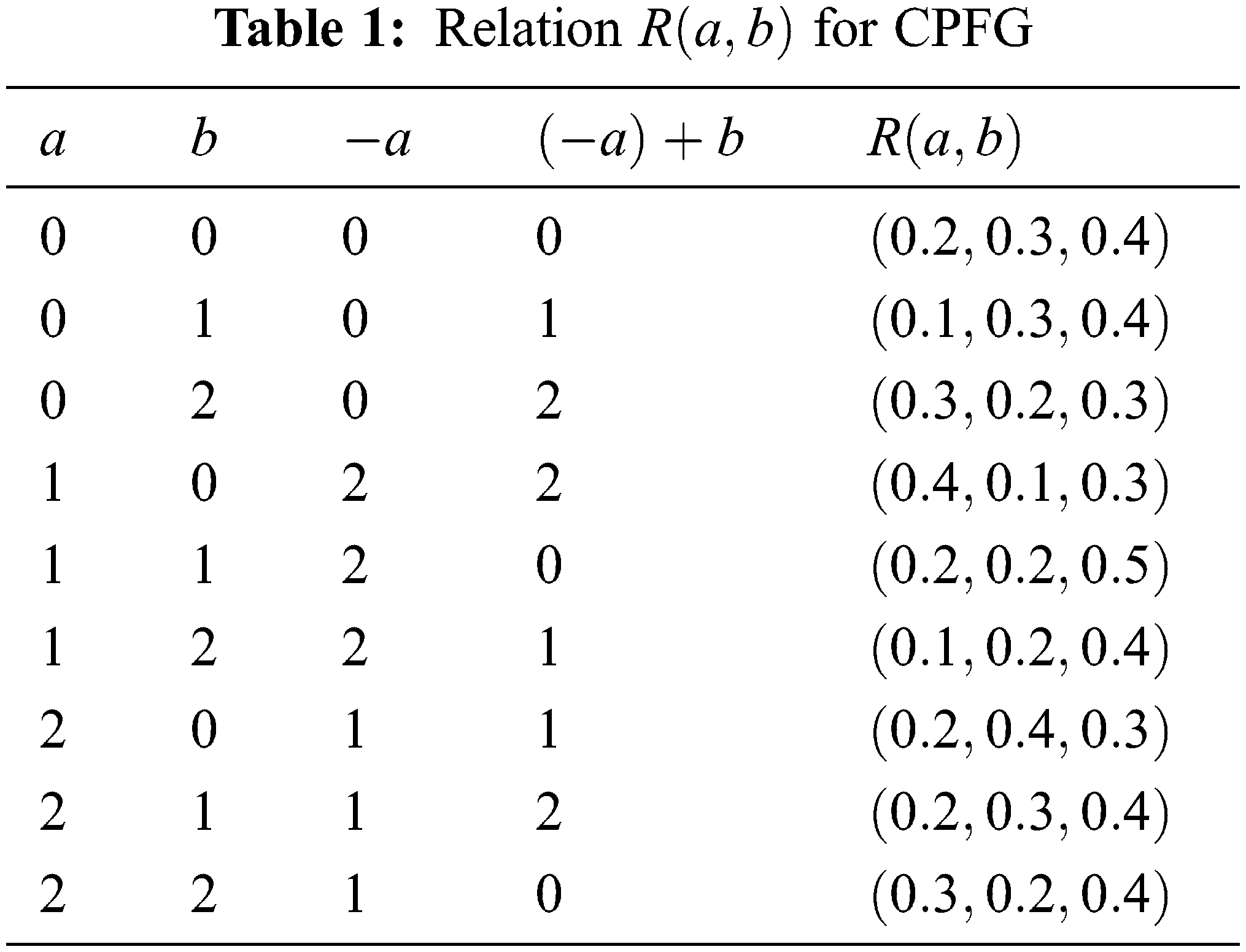
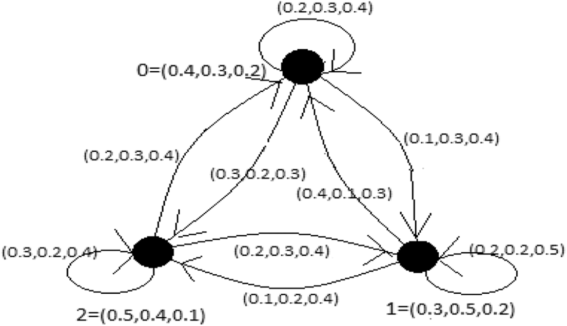
Figure 1: Cayley picture fuzzy graph

Definition 10. Let G be Cayley picture fuzzy directed graph. Then the in degree (ind) of a node or vertex a in G is defined as ind(a)=(indξA(a),indρA(a),indωA(a)) , where indξA(a)=∑b≠aΥR(ab−1) , indρA(a)=∑a≠bϕA(ab−1) and indωA(a)=∑b≠aψR(ab−1) . Similarly, the out degree (out) of a vertex a in G is defined by out(a)=(outξA(a),outρA(a),outωA(a)) , where outξA(a)=∑b≠aΥR(ab−1) , outρA(a)=∑b≠aϕR(ab−1) and outωA(a)=∑b≠aψR(ab−1) .

Remark 1. A Cayley picture fuzzy directed graph having equal out (resp., in) degree r for every vertex is said to be out (resp., in) regular directed graph with the index of out (resp., in) regularity r .

Example 2. The graph given in Fig. 1 is a regular CPFG.

Theorem 1. Every CPFG is vertex transitive.

Proof. Let G=(A,R) be a CPFG, where A=(ξA,ρA,ωA) and R=(ΥR,ΦR,ψR) defined on G=(V,E) . Let m,n∈V . Define α:V→V as α(x)=nm−1x ∀ x∈V . Then, for all x,y∈V α is a bijective map. Consider R(α(x),α(y)) = (RΥ(α(x), α(y)), Rϕ(α(x), α(y)), Rψ(α(x), α(y))). For this,

(i) RΥ(α(x),α(y)) = RΥ(nm−1x,nm−1y) = ΥA((nm−1x)−1(nm−1x)) = ΥA(x−1y) = RΥ(x,y)

(ii) Rϕ(α(x),α(y)) = Rϕ(nm−1x,nm−1y) = ϕA((nm−1x)−1(nm−1x)) = ϕA(x−1y) = Rϕ(x,y)

(iii) Rψ(α(x),α(y)) = Rψ(nm−1x,nm−1y) = ψA((nm−1x)−1(nm−1x)) = ψA(x−1y) = Rψ(x,y).

From (i), (ii) & (iii) we get R(α(x),α(y)) = R(x,y) . Therefore, α is an automorphism on group and α(a)=b . Hence CPFGs is vertex transitive.

Theorem 2. Every vertex transitive CPFG is regular.

Proof. Let G=(A,R) be a vertex transitive CPFG, where A=(ξA,ρA,ωA) and R=(ΥR,ΦR,ψR) defined on G=(V,E) and let u,v∈V. The automorphism f on group is f(u)=v. Note that ind(u) = ∑x∈VR(x,u) = ∑x∈V(RΥ(x,u), Rϕ(x,u), Rψ(x,u)) = ∑x∈V((RΥ(f(x),f(u)), Rϕ(f(x),f(u)), Rψ(f(x),f(u))) = ∑x∈V((RΥ(f(x),v), Rϕ(f(x),v), Rψ(f(x),v)) = ∑x∈V(RΥ(y,v), Rϕ(y,v), Rψ(y,v)) = ind(v)

Similarly,

out(u) = ∑x∈VR(x,u) = ∑x∈V((RΥ(u,x), Rϕ(u,x),Rψ(u,x)) = ∑x∈V((RΥ(f(u),f(x)), Rϕ(f(u),f(x)), Rψ(f(u),f(x))) = ∑x∈V((RΥ(v,f(x)), Rϕ(v,f(x)), Rψ(v,f(x))) = ∑x∈V((RΥ(v,y), Rϕ(v,y), Rψ(v,y)) = outd(v).

Thus, G is regular.

4  Cayley Graphs Induced by Cayley Picture Fuzzy Graphs

In this section, first we introduce α, β, γ− cuts of CPFG and then we obtain the linkage between a CPFGs and its corresponding crisp graphs by using these cuts.

Definition 11. Let G∗=(V,E) be a Cayley graph, where V=(G,∗) be a group. Let G=(A,R) be a CPFG on G∗ , where A is a CPF subset of V and R is a CPF relation defined on E ⊆ V×V. Now A=(u:ξA(u),ρA(u),ωA(u)) and R(a,b) = {(uv : ΥR(u−1v), ϕR(u−1v), ψR(u−1v)) | u,v∈G and u−1v∈T} . Then the level set of A is defined as

LA={α:ξA(u)=α,α∈[0,h1]}∪{β:ρA(u)=β,β∈[h2,1]}∪{γ:ωA(u)=γ,γ∈[h3,1]}.

A level set of R is defined as

LR={α:ΥR(u−1v)=α,α∈[0,t1]}∪{β:ϕR(u−1v)=β,β∈[t2,1]}∪{γ:ψR(u−1v)=γ,γ∈[t3,1]}

where h1,h2,h3 and t1,t2,t3 are heights of positive memberships, negative memberships and neutral memberships of A and R , respectively, A level set of a CPFG is the set L=LA∪LR.

Definition 12. Let G∗=(V,E) be a Cayley graph, where V=(G,∗) be a group and let T≠ ∅ be a subset of (G,∗) . Let G=(A,R) be a CPFG on G∗ , where A=(ξ,ρ,ω) is a CPF subset of V and R=(Υ,Φ,Ψ) is a CPF relation defined on E ⊆ V×V. Given α, β, γ∈L ∪{0} , where L is level set of the CPFG and α + β + γ≤1 . And α, β, γ− cuts of a graph G is a crisp graph G∗(α,β,γ) = (VLα,β,γ,ELα,β,γ) for which

VLα,β,γ={x∈V:ξA(x)≥α,ρA(x)≥β,ωA(x)≤γ}and

ELα,β,γ={ΥR(x−1y)≥α,ΦR(x−1y)≥β,ΨR(x−1y)≤γandx,y∈G,x−1y∈T}.

Theorem 3. Let G∗=(V,E) be a Cayley Graph, where V is a group. Let G=(A,R) be a CPFG defined on G∗, where A=(x,ξA(x),ρA(x),ωA(x)) and R={(x,y : ΥR(x−1y), ΦR(x−1y), ΨR(x−1y)) : x,y∈G x−1y∈T} . Given α1, β1 , γ1 ; α2, β2, γ2 ∈L , where L is a level set of CPFG and α1 + β1 + γ1 ≤1 , α2 + β2 + γ2 ≤1 . If α1 ≥ α2, β1 ≥ β1, γ1 ≤ γ2, then

Gα1+β1+γ1⊆Gα2+β2+γ2.

Proof. Let α1, β1, γ1 ; α2, β2, γ2 ∈L . Let x be any vertex in VLα,β,γ. Following the definition of a level set of the CPFG, we have ξA(x) ≥ α1, ρA(x) ≥ β1, ωA(x) ≤ γ1 . Let xy be any edge in ELα,β,γ . It means that ΥR(x−1y) ≥ α1, ΦR(x−1y) ≥ β1, ΨR(x−1y) ≤ γ1. We know that α1 ≥ α2, β1 ≥ β2, γ1 ≤ γ2. It implies ξA(x) ≥ α1 ≥ α2 , ρA(x) ≥ β1 ≥ β2 , ωA(x) ≤ γ1 ≤ γ2 and ΥR(x−1y) ≥ α1 ≥ α2 , ΦR(x−1y) ≥ β1 ≥ β2 , ΨR(x−1y) ≤ γ1 ≤ γ2. We obtain x∈ VLα2,β2,γ2 and xy∈ ELα2,β2,γ2 . Therefore, ALα1,β1,γ1 ⊆ ALα2,β2,γ2 and RLα1,β1,γ1 ⊆ RLα2,β2,γ2 . Hence Gα1,β1,γ1 ⊆ Gα2,β2,γ2.

Theorem 4. Given a CPFG G=(A,R) on Cayley Graph G∗=(V,E) and let T≠∅ be a subset of V=G . If α=0, β=0, γ = max {d1,d2} , where d1= max {ω(x):x∈V} and d2= max {Ψ(x−1y):x,y∈G,x−1y∈T}, then the cut Gα,β,γ of the CPFG is a complete Cayley graph.

Proof. Since α=0, β=0, γ= max {d1,d2} , for each x in A satisfying ξA(x) ≥ α, ρA(x) ≥ β, ωA(x) ≤ γ . Also, all pairs uv for every v,u ∈G satisfying ΥR(x−1y) ≥ α, ΦR(x−1y) ≥ β, ΨR(x−1y) ≤ γ. Hence, the (α,β,γ)− cut of the CPFG is a crisp graph in which there is a connection between each pair of its vertices. Hence the cut is a (crisp) Cayley complete graph.

Theorem 5. Let G=(A,R) be a CPFG defined on a Cayley Graph G∗=(V,E) and let T≠∅ be a subset of a group G=V . Let A=(ξA(x),ρA(x),ωA(x)) and R={(x,y) : ΥR(x−1y), ΦR(x−1y), ΨR(x−1y)) : x,y∈G x−1y∈T}. Let a = min {ξA(x) }, b = min {ΥR(x−1y)} , c1 = min {ρA(x)} , c2 = min {ϕR(x−1y)} , d1 = max {ωA(x)} , d2 = max {ψR(x−1y)} . If α = min (a,b), β = min (c1,c2), γ = max (d1,d2), then the cut Gα,β,γ of a CPFG is a Cayley graph G∗ .

Proof. Since α = min (a,b), β = min (c1,c2), and γ = max (d1,d2), we get ξ(x) ≥ α, ρ(x) ≥ β, ω(x) ≤ γ for each x∈A . Also, each pair xy∈E is satisfying ΥR(x−1y) ≥ α, ΦR(x−1y) ≥ β, ΨR(x−1y) ≤ γ. Thus, all the vertices and edges of the CPFG G are lying in the cut G∗(α,β,γ) . Hence the cut is the underlying Cayley graph G∗=(V,E).

5  Vertex and Edge Connectivity in CPFGs

The terms vertex connectivity and edge connectivity of a fuzzy graphs have been introduced in [31]. The notion of strong edges (arcs) in fuzzy graphs was initiated in [33]. These terms were further generalized in [32]. Throughout this section, we shift these terminologies towards PFGs and CPFGs. We divide this section into three subsections. In Section 1, we discuss the notion of the vertex connectivity of a CPFGs. Section 2 is devoted for discussion on the edge connectivity of the CPFGs. In the third subsection, we explore the relationship between vertex and edge connectivity of the CPFGs.

5.1 Vertex Connectivity in CPFGs

We present the definitions of disconnection and vertex connectivity of PFGs (resp., CPFGs) which are due to the work presented in [31–33] for fuzzy graphs.

Definition 13. A disconnection of a PFG G=(A,R) is a vertex set D whose removal results in a disconnection or a single vertex of PFG. The weight of D may be described by ∑v∈D( min ΥR(uv), min ϕR(uv), max ψR(uv)).

Remark 2. In the above definition, if G is a CPFG then the weight of D is

∑v∈D(minΥR(uv−1),minϕR(uv−1),maxψR(uv−1)).

Definition 14. The vertex connectivity of a CFG (resp., CPFG) G is the minimum weight of a disconnection in G and is denoted by Ω(G).

Let G be a PFG. Then, if we exempt the vertex vi in G such that it decreases the strength of the connectedness among some pairs of vertices, then we say it a cut vertex of G .

Definition 15. Let G=(A,R) be a connected PFG (resp., CPFG). A set of vertices X = {v1, v2, v3, …, vm} ⊂ A∗=(ξ∗,ρ∗,ω∗) is said to be a PFG vertex cut (in short, PFGVC (resp., CPFGVC)) if either CONNG−X(a,b) < CONNG(a,b) , CONNG−X(a,b) < CONNG(a,b) and CONNG−X(a,b) > CONNG(a,b) , for some pairs of the vertices a,b belongs to ( ξ∗ , ρ∗ , ω∗ ), respectively, such that both a,b ≠ vi for i = 1, 2, …, m or G−X is trivial.

Example 3. Let G=(A,R) be a CPFG, where A is a picture fuzzy set defined on a group V4=A={e,a,b,ab}, and R=(ΥR(uv−1), ϕR(uv−1), ψR(uv−1)), here ΥR(ea−1) = ΥR(abb−1) = 0.1, ΥR(ab−1) = 0.15, ΥR(aba−1) = ϕR(ea−1) = ϕR(ab−1) = 0.2, ϕR(aba−1) = ϕR(abb−1) = 0.2 and ψR(ea−1) = ψR(ab−1) = 0.4, ψR(abb−1) = 0.3, ψR(aba−1) = 0.4.

Then S={ab,b} is a 2-CPFNC for, CONNG−S(a−1e) = 0.1 < 0.2 = CONNG(a−1e) , CONNG−S(a−1e) = 0.1 < 0.3 = CONNG(a−1e) and CONNG−S(a−1e) = 0.4 > 0.3 = CONNG(a−1e) . Also disconnection can be calculated by D = ∑V∈D( min ΥR(ab−1), min ϕR(ab−1), max ψR(ab−1)).

Picture fuzzy vertex cuts of G are ab , b and a with strong weights D(ab) = (0.4, 0.3, 0.1), D(b) = (0.2, 0.4, 0.3) and D(a) = (0.6, 0.7, 0.4). Thus the vertex connectivity is as follows.

Ω(G)=(min(D(ab),D(b),D(a)),min(D(ab),D(b),D(a)),max(D(ab),D(b),D(a)))=(min(0.4,0.2,0.6),min(0.3,0.4,0.7)max(0.1,0.3,0.4))=(0.2,0.3,0.4).

5.2 Edge Connectivity in CPFGs

Definition 16. Let G be a CPFG graph and {V1,V2} be the partition of its set of vertices. The edges set joining the vertices of V1 and vertices of V2 is said to be a cut-set of G relative to the partition {V1,V2} and is denoted by (V1,V2). The weight of the cut-set (V1,V2) is described by D′ = ∑u∈V1,v∈V2( ΥR(ab−1), ϕR(ab−1), ψR(ab−1)).

Definition 17. The minimum weight of cut-sets of a PFG (resp., CPFG) G is the edge connectivity of G and is denoted by λ(G) .

Definition 18. An edge of a PFG (resp., CPFG) G is said to be a strong edge, if its weight is at least as great as the connectedness of its end vertices, whenever it is removed.

Definition 19. Let G=(C,D) be a connected CPFG. A set of strong edges E = {e1, e2, e3, …, em} with ei = (ui,vi), i = 1, 2, …, n is said to be a CPFG-edge cut (CPFGEC) if either CONNG−E(a,b) < CONNG(a,b) , CONNG−E(a,b) < CONNG(a,b) and CONNG−E(a,b) > CONNG(a,b) such that a,b ∈G and a−1b∈T, for some pair of vertices a,b belongs to ( ξ∗ , ρ∗ , ω∗ ) with at least one of a or b is different from both ui and vi , i = 1, 2, …, n , or G−E is disconnected.

If there are n edges in E then we say it is an n -CPFGECs. Among the others CPFG edge cuts the CPFG edge cut with one edge (1-CPFGEC) is the special type and we call it a CPF-bridge.

Definition 20. A 1-CPFGEC is a CPFGEC bond (CPFGEC-bond).

Remark 3. If (u,v) is a bridge in any graph, then at least one of u or v must be a cut-node. However, in CPFG, if (u,v) is a CPF bridge, it is not necessary that at least one of u or v is a CPFGC vertex.

Proposition 1. In a CPFG-bond of a CPFG there is at least one of the end nodes of a CPFG-bond is a CPFG-cut vertex.

Proof. Let G=(A,R) be a CPFG and let e=(u,v) be an CPFG-bond in G. Since e is a CPFG-bond, by deleting e from G decreases the strength of connectedness between x and y such that at least one of them is different from u and v . However, if both x and y are different from u and v , then u as well as v will become a CPFGC-vertex. On the other hand, if one of x or y coincides with u or v , then u or v which is neither x nor y will be a CPFGC-vertex.

Example 4. Let G=(A,R) be a CPFG, where A is a picture fuzzy set defined on a group V4=A={e,a,b,ab}, and R=(ΥR(uv−1), ϕR(uv−1), ψR(uv−1)) , where ΥR(ea−1) = ΥR(abb−1) = 0.1, ΥR(ab−1) = 0.15, ΥR(abb−1) = ΥR(eab−1) = 0.1, ϕR(ea−1) = 0.05, ϕR(ea−1) = ϕR(ab−1) = 0.2, ϕR(aba−1) = ϕR(abb−1) = 0.2 and ψR(ea−1) = ψR(ab−1) = 0.4, ψR(abb−1) = 0.3, ψR(aba−1) = 0.4, ψR(ea−1) = 0.3. There are three CPF bonds(1-CPFEC) namely the edges (a, e), (a, b) and (b, ab). Also E = {(a, b), (e, ab)} is a 2-CPFEC, since 0.1= CONNΥR(G)−E(b−1e) < CONNΥR(G)(b−1e) = 0.15, 0.1 = CONNϕR(G)−E(b−1e) < CONNϕR(G)(b−1e) = 0.15 and 0.5 = CONNψR(G)−E(b−1e) > CONNψR(G)(b−1e) = 0.3. Then the strong weight of E={(e,a), (a,b)} and edge connectivity can be calculated as follows.

D′(e)=(0.2,0.1.0.2),D′(ea−1)=(0.1,0.1.0.5),D′(ab−1)=(0.15,0.2,0.4)

λ(G)={min(0.2,0.1,0.15),min(0.1,0.1,0.2),max(0.2,0.5,0.4)}=(0.1,0.1,0.5)

5.3 Relationship between Vertex Connectivity and Edge Connectivity in CPFGs

Definition 21. A CPFG G=(C,D) is a CPF tree if it has an CPF spanning subgraph H=(E,F) which is a tree, where for all edges (u,v) not in H, ΥR(a−1b) = ∧ {ΥF((a−1)b)} , ϕR(a−1b) = ∧ {ϕF((a−1)b)} and ψR(a−1b) = ∨ {ψF((a−1)b)} : a,b ∈G and a−1b∈T.

Theorem 6. In a CPF tree of a graph G=(A,R)

Ω(G)=λ(G)={∧(γR(x−1y)),∀xy∈G,x−1y∈T∧(ϕR(x−1y)),∀xy∈G,x−1y∈T∨(ψR(x−1y))∀xy∈G,x−1y∈T (1)

such that x−1y is a strong edge in G.

Proof. Let G=(A,R) be a CPF tree. Assume that F=(A,S) is a unique maximum spanning CPF tree of G . An edge (x−1y) in G=(A,R) is an CPF-bridge if and only if (x−1y) is an edge of maximum spanning CPF tree F of G. Such CPF-bridges are CPF-bonds, also the edges in F are strong edges. Hence every strong edge in F is a 1-CPF cut of G. Evidently, a strong weight of each such 1-CPFC is {γR(x−1y), ϕR(x−1y), ψR(x−1y)}. Thus, CPFG edge connectivity λ(G) is the minimum weight of all edges in F and therefore the minimum weight of all strong edges in G.

Now every internal vertex of F is an F-cut vertex of CPF tree of G and hence are 1-CPFG vertex cut of G. Hence CPFG vertex connectivity Ω(G) is the minimum weight of all vertices in F and hence is a minimum weight of all strong edges in G. Which completes the proof.

However, in a common CPFG, Theorem 13 does not hold true as we observe in Example 5.

Example 5. From Examples (3 & 4), we have observed the followings.

Ω(G)=(min(0.4,0.2,0.6),min(0.3,0.4,0.7)max(0.1,0.3,0.4))=(0.2,0.3,0.4)

λ(G)={min(0.2,0.1,0.15),min(0.1,0.1,0.2),max(0.2,0.5,0.4)}=(0.1,0.1,0.5).

Which implies Ω(G) ≠ λ(G) .

6  Application

Due to the current progress of parallel and distributed computing, the design and analysis of diverse interconnected networks have been a significant area of research for the last few years and is still triggered by the new technologies introduced in the field of communication networking like optic fibers. In this regard, various classes of Cayley graphs are used in the modeling of interconnected networks and routings. Since the signals in such systems within the range can either be connected, disconnected or fluctuate between the positions of connected and disconnected. It is well known that in any network environment the data transferred across the network in the shape of packets. However, these packets are interrupted during their journey due to network congestion, overtaxed devices, software bugs and so on. Generally, the wireless networks face more issues with packet loss than the wired networks as the weaker signals, radio frequency interference, physical barriers and distance are the main reasons of wireless networks to drop packets. Hence the modelling of interconnected networks in the setting of fuzzy graphs is more practical. Specifically, as CPFGs is a vertex transitive so it is most suitable to describe interconnected networks. We present such model through a CPFG shown in Fig. 2.

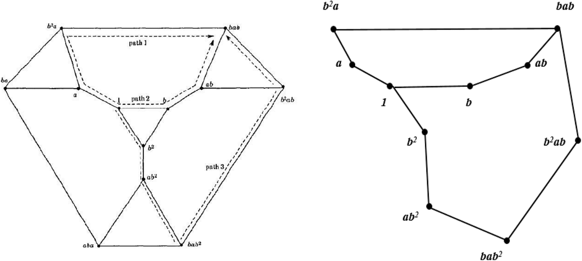
Figure 2: Cayley picture fuzzy graph defined on A4

From Fig. 2 and its description, it is evident that the level of communication between and a is better than that of b2a and bab and so on.

Similarly, we may describe the levels of the vertex and edge connectivity of the interconnected networks given in Fig. 2. For this, let V1 and V2 be two partitions of vertex set V , where V1 = {1,a,ba,bab,ab,b} and V2 = {1,b2,ab2,bab2,b2ab,bab}. Here V1 consists of two paths P1 and P2 while V2 consists of a path P3. Disconnection (D) in V2 consists of {1,a,ba,bab} and {1,b,ab,bab} . We can easily calculate D = ∑V∈D( min ΥR(uv−1), min ϕR(uv−1), max ψR(uv−1)) and D′ = ∑u∈V1,v∈V2( ΥR(uv−1), ϕR(uv−1), ψR(uv−1)). Finally, the vertex connectivity and edge connectivity of the graph shown in Fig. 2 can be easily calculated. For this, we describe the following cases:

References

1.  L. Zadeh, “Fuzzy sets,” Information and Control, vol. 8, no. 3, pp. 338–353, 1965. [Google Scholar]
2.  L. Zadeh, “The concept of a linguistic variable and its application to approximate reasoning—I,” Information Science, vol. 8, no. 3, pp. 199–249, 1975. [Google Scholar]
3.  K. T. Atanassov, “Intuitionistic fuzzy sets,” Fuzzy Sets and Systems, vol. 20, pp. 87–96, 1986. [Google Scholar]
4.  T. Chaira and A. K. Ray, “A new measure using intuitionistic fuzzy set theory and its application to edge detection,” Applied Soft Computing, vol. 8, no. 2, pp. 919–927, 2008. [Google Scholar]
5.  D. F. Li, “Multiattribute decision making models and methods using intuitionistic fuzzy sets,” Journal of Computer and System Sciences, vol. 70, no. 1, pp. 73–85, 2005. [Google Scholar]
6.  B. C. Cuong and V. Kreinovich, “Picture fuzzy sets,” Journal of Computer Science and Cybernetics, vol. 30, no. 4, pp. 409–420, 2014. [Google Scholar]
7.  P. H. Phong, D. T. Hieu, R. Ngan and P. T. Them, “Some compositions of picture fuzzy relations,” in Proc. of the 7th National Conf. on Fundamental and Applied Information Technology Research (FAIR’7), Thai Nguyen, Vietnam, 19–20 June 2014, pp. 19–20, 2014. [Google Scholar]
8.  B. C. Cuong and V. H. Pham, “Some fuzzy logic operators for picture fuzzy sets,” in Proc. of the 2015 Seventh Int. Conf. on Knowledge and Systems Engineering (KSE), Ho Chi Minh City, Vietnam, 8–10 2015, pp. 132–137, 2015. [Google Scholar]
9.  G. Wei, “Some cosine similarity measures for picture fuzzy sets and their applications to strategic decision making,” Informatica, vol. 28, no. 3, pp. 547–564, 2017. [Google Scholar]
10. A. M. Khalil, S. G. Li, H. Garg, H. Li and S. Ma, “New operations on interval-valued picture fuzzy set, interval-valued picture fuzzy soft set and their applications,” IEEE Access, vol. 7, pp. 51236–51253, 2019. [Google Scholar]
11. A. Rosenfeld, “Fuzzy graphs,” in Fuzzy Sets and Their Applications to Cognitive and Decision Processes, L. A. Zadeh, K. S. Fu, K. Tanaka, M. Shimura (eds.New York: Academic Press, pp. 77–95, 1975. [Google Scholar]
12. J. N. Mordeson and P. S. Nair, “Fuzzy graphs and fuzzy hypergraphs,” in Studies in Fuzziness and Soft Computing. Springer-Verlag Berlin GmbH, 2000. [Google Scholar]
13. M. Sunitha and A. Vijayakumar, “Complement of a fuzzy graph,” Indian Journal of Pure and Applied Mathematics, vol. 33, no. 9, pp. 1451–1464, 2002. [Google Scholar]
14. R. Parvathi and M. Karunambigai, “Intuitionistic fuzzy graphs,” in Journal of Computational Intelligence: Theory and Applications. Berlin, Heidelberg: Springer, pp. 139–150, 2006. [Google Scholar]
15. A. Shannon and K. T. Atanassov, “On a generalization of intuitionistic fuzzy graphs,” Notes on Intuitionistic Fuzzy Sets, vol. 12, no. 1, pp. 24–29, 2006. [Google Scholar]
16. S. Thilagavathi, R. Parvathi and M. Karunambigai, “Operations on intuitionistic fuzzy graphs II,” In: International conference in International Journal of Computer Applications, vol. 51, 2009. [Google Scholar]
17. M. Akram and R. Akmal, “Operations on intuitionistic fuzzy graph structures,” Fuzzy Information and Engineering, vol. 8, no. 4, pp. 389–410, 2016. [Google Scholar]
18. H. Rashmanlou, S. Samanta, M. Pal and R. A. Borzooei, “Intuitionistic fuzzy graphs with categorical properties,” Fuzzy Information and Engineering, vol. 7, no. 3, pp. 317–334, 2015. [Google Scholar]
19. S. Sahoo and M. Pal, “Different types of products on intuitionistic fuzzy graphs,” Pacific Science Review A: Natural Science and Engineering, vol. 17, no. 3, pp. 87–96, 2015. [Google Scholar]
20. M. Akram and W. A. Dudek, “Intuitionistic fuzzy hypergraphs with applications,” Information Sciences, vol. 218, pp. 182–193, 2013. [Google Scholar]
21. M. Karunambigai, P. Rangasamy, K. T. Atanassov and N. Palaniappan, “An intuitionistic fuzzy graph method for finding the shortest paths in networks,” in Theoretical Advances and Applications of Fuzzy Logic and Soft Computing. Berlin, Germany: Springer, pp. 3–10, 2007. [Google Scholar]
22. D. Yu and S. Shi, “Researching the development of Atanassov intuitionistic fuzzy set: Using a citation network analysis,” Applied Soft Computing, vol. 32, no. 1, pp. 189–198, 2015. [Google Scholar]
23. M. Akram, M. Karunambigai and O. Kalaivani, “Cayley intuitionistic fuzzy graphs,” Journal of Applied Mathematics and Informatics, vol. 32, no. 5–6, pp. 827–842, 2014. [Google Scholar]
24. C. Zuo, A. Pal and A. Dey, “New concepts of picture fuzzy graphs with application,” Mathematics, vol. 7, no. 5, pp. 470, 2019. [Google Scholar]
25. S. Das and G. Ghorai, “Analysis of road map design based on multigraph with picture fuzzy information,” International Journal of Applied and Computational Mathematics, vol. 6, no. 3, pp. 1–17, 2020. [Google Scholar]
26. R. Anjum, A. Gumaei and A. Ghaffar, “Certain notions of picture fuzzy information with applications,” Journal of Mathematics, vol. 2021, no. 3, pp. 1–8, 2021. [Google Scholar]
27. S. Amanathulla, B. Bera and M. Pal, “Balanced picture fuzzy graph with application,” Artificial Intelligence Review, vol. 54, no. 7, pp. 5255–5281, 2021. [Google Scholar]
28. W. A. Khan, B. Ali and A. Taouti, “Bipolar picture fuzzy graphs with application,” Symmetry, vol. 13, no. 8, pp. 1427, 2021. [Google Scholar]
29. W. A. Khan, K. Faiz and A. Taouti, “Interval-valued picture fuzzy graphs,” in Demonstratio Mathematica, 2021. [Google Scholar]
30. K. T. Atanassov, “Intuitionistic fuzzy sets,” Fuzzy Sets and Systems, vol. 20, no. 1, pp. 87–96, 1986. [Google Scholar]
31. R. T. Yeh and S. Bang, “Fuzzy relations, fuzzy graphs, and their applications to clustering analysis,” in Fuzzy Sets and Their Applications to Cognitive and Decision Process, L. A. Zadeh, K. S. Fu, M. Shimura (eds.New York, NY, USA: Academic Press, pp. 338–353, 1975. [Google Scholar]
32. S. Mathew and M. Sunitha, “Node connectivity and arc connectivity of a fuzzy graph,” Information Sciences, vol. 180, no. 4, pp. 519–531, 2010. [Google Scholar]
33. K. R. Bhutani and A. Rosenfeld, “Strong arcs in fuzzy graphs,” Information Sciences, vol. 152, pp. 319–322, 2003. [Google Scholar]
Cite This Article
APA Style
Khan, W.A., Faiz, K., Taouti, A. (2023). Cayley picture fuzzy graphs and interconnected networks. Intelligent Automation & Soft Computing, 35(3), 3317-3330. https://doi.org/10.32604/iasc.2023.024484
Vancouver Style
Khan WA, Faiz K, Taouti A. Cayley picture fuzzy graphs and interconnected networks. Intell Automat Soft Comput . 2023;35(3):3317-3330 https://doi.org/10.32604/iasc.2023.024484
IEEE Style
W.A. Khan, K. Faiz, and A. Taouti "Cayley Picture Fuzzy Graphs and Interconnected Networks," Intell. Automat. Soft Comput. , vol. 35, no. 3, pp. 3317-3330. 2023. https://doi.org/10.32604/iasc.2023.024484
cc This work is licensed under a Creative Commons Attribution 4.0 International License , which permits unrestricted use, distribution, and reproduction in any medium, provided the original work is properly cited.
• 830
View
• 411
Download
• 0
Like
Related articles