Cephalopods Classification Using Fine Tuned Lightweight Transfer Learning Models

1  Introduction

Marine molluscs are a distinct class of creatures with more than 100,000 diverse classes presently. Cephalopods are the members of the mollusc phylum encompassing fewer than 1000 classes scattered in 43 families [1]. Cephalopod has seized to grow steadily in the last four decades. According to food and agricultural organization, the catching of cephalopods has increased from 1 million metric tonnes to 3.6 million metric tonnes.

The most extravagant species in the Indian market are those rapports to cuttlefish and squid [2,3]. This experience makes to have approaches for classifying cephalopod species, despite morphological characteristics that have been evacuated. Earlier cephalopods are classified using biochemical and molecular taxonomic markers [4,5]. The molecular taxonomy of cephalopods is highly expensive and time-consuming, so there is a need for an alternative tool. This study focuses on developing an automated system that classifies and separates the cephalopod species into different categories.

Deep Learning (DL) techniques have recently been used to solve various classification problems in robotics, sports, and medicine [6–9]. The most prevalent deep learning models [10] are Convolutional Neural Networks (CNNs), which offer a lot of potential for the classification of tasks [11]. Salman et al. [12] had created a deep network to classify undersea species of fish. Deep learning involves an extensive dataset and a lot of computing power, leading to overfitting in small datasets [13].

Allken et al. [14] suggested a strategy for increasing the training sample based on a rational deep vision picture simulation to compensate for the lack of labeled data, reaching a categorization rate of 94% for Atlantic herring, blue whiting, and Atlantic mackerel. A method based on cross-convolutional layer pooling on a pre-trained CNN was presented in [15] to avoid the requirement for a significant quantity of training data. A validation accuracy of 98.03% was found after a thorough analysis of 27,370 species of images.

Xu et al. [16] also reported the species recognition based on SE-ResNet152 and class-balanced focal loss. The marine fish Tuna was similarly classified using a region-based CNN with ensembling [17]. When tested with an independent test dataset, the proposed approach achieved a precision of 93.91%. Based on this, Iqbal et al. [18] presented a model which employed a simplified AlexNet model with four convolutional layers and two fully connected layers.

It is demonstrated to be advantageous that use of sample expansion and transfer learning methodologies to improve the learning model generalization and mitigate the problem of limited sample data overfitting. Furthermore, the optimal model structure for various target datasets usually is different. An automatic cephalopods identification method is proposed using the transfer learning approach based on the issues. A network with very little weight is necessary to enable an IoT device or any embedded devices [19,20] to recognize cephalopod images automatically. The following is a list of contributions to the present research.

•   For the novel cephalopod image classification, in this study, lightweight pre-trained models (Slim Networks) are being used. Furthermore, the models are fine-tuned for improving the accuracy of classification.

•   An optimizer is proposed to boost the accuracy rates further while reducing the training time.

•   The models are tested, and the performance of the models is compared to select the ideal candidates for integration in embedded or IoT devices for cephalopod species classification.

The following sections are laid out as follows; Data sources for this article and the pre-trained models are discussed in Section 2. Section 3 presents the results of the tests, the specifics of the suggested optimizer, and interpretations of the findings. Section 4 wraps up the results presented in this paper.

2  Materials and Methods

2.1 Image Collection

A Canon EOS 1000D was used to capture the cephalopod images in this dataset with a resolution of 10.1 effective megapixels, 3,888 × 2,592, from Kasimedu and Tuticorin coastal areas of Bay of Bengal. Six common species of cephalopods, namely Sepia pharaonis, Sepia prashad, Sepia aculeata, Sepioteuthis lessoniana, Uroteuthis duvauceli, and Doryteuthis siboga are collected and used in the proposed work. Field and sample images are shown in Fig. 1. The selected species of cephalopods are found all over India, and their reproduction speed is also high.

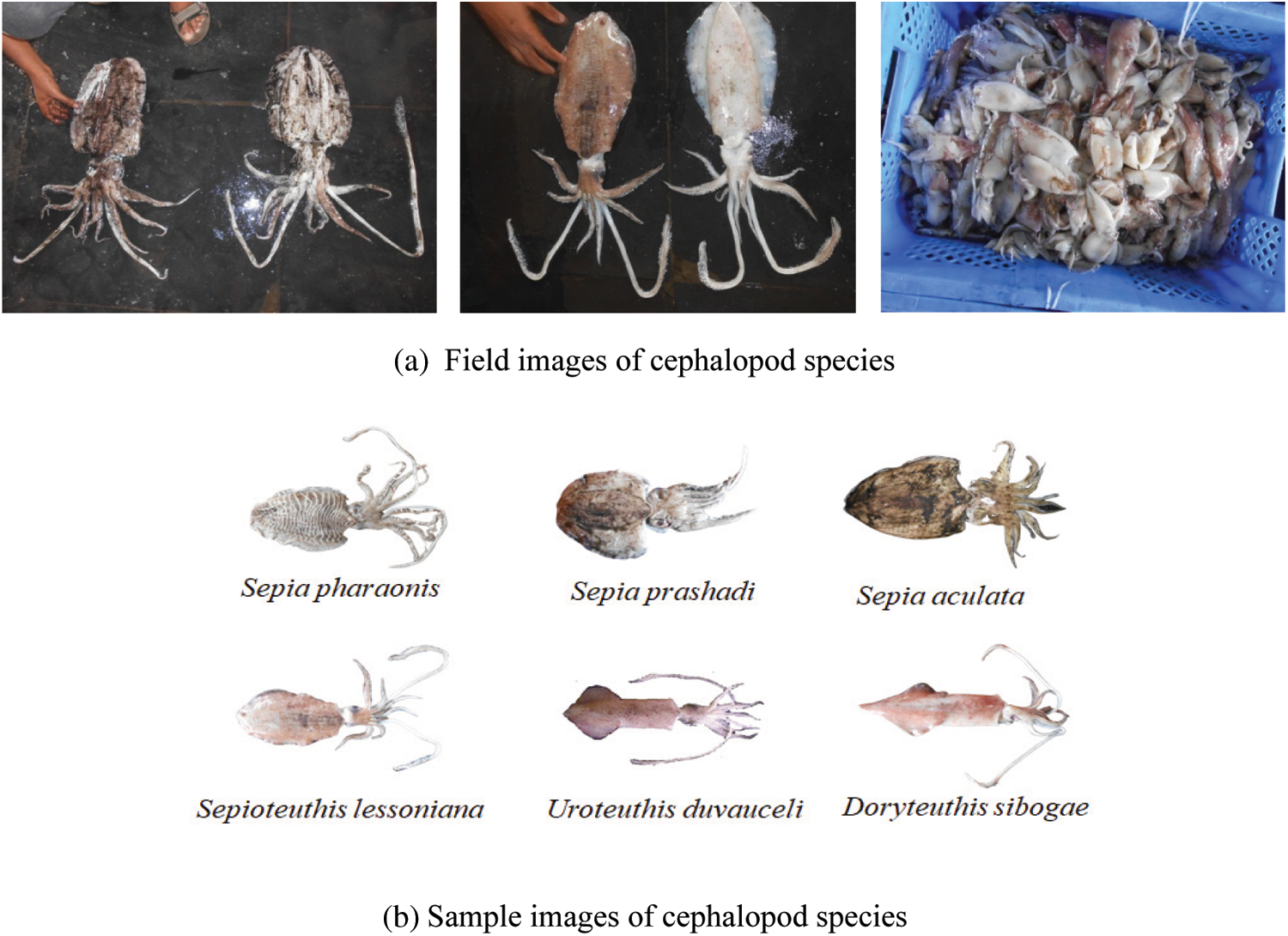
Figure 1: (a) Field images of cephalopod species (b) Sample images of cephalopod species

These six species are noteworthy in terms of classification study. Totally, 492 images (D. sibogae, 84; S. aculeata, 88; S. pharaonis, 80; S. Prashad, 88; S. lessoniana, 78; U. duvauceli, 74) have been collected from the coastal areas. With these photographs, a new cephalopod image dataset is created. The newly created dataset is used for the first time in the proposed work.

2.2 Image Augmentation and Scaling

Data augmentation was used in the proposed study to address the overfitting issues by increasing the base data set and implementing the label-preserving transformations [21]. The following transformation operations were used to expand the dataset. The methods uniform distribution, rotating images at random within a precise range were used. Images were shifted vertically and horizontally by a random percentage of their total size. A part of the pictures was flipped horizontally, then arbitrary scaling and shearing changes were done. Image data generator [22] accepts batches of images and transforms them into a new set of images at random. Before being applied to any model, the image of size 4608 × 3456 is scaled down to size 224 × 224.

2.3 Proposed System for Cephalopod Classification

2.3.1 Fine Tuned MobileNetV2 Architecture

The MobileNet model focuses on depthwise separable convolutions, a factorized convolution that splits a standard convolution into a depth-wise and a pointwise convolution. The depth-wise convolution used by Mobile Nets utilizes a single filter for each input channel. The outputs of depth-wise convolution are then combined using an 1 × 1 convolution by pointwise convolution. This is divided into two layers by the depthwise separable convolutions; one for filtering and the other for connecting. This factorization has the benefit of significantly lowering the computing time. An improved module with an inverted residual structure has been added to MobileNetV2 [23]. The first layer is 1 × 1 convolution with Rectified Linear Unit (ReLU). The depthwise convolution is the second layer. Another 1 × 1 convolution is used in the third layer with no non-linearity. Deep networks will only have the power of a linear classifier on the non-zero volume output domain if ReLU is applied again.

The projection layer, a pointwise convolutional layer in V2, converts the data with many channels into a tensor with much fewer channels. Before going into the depth-wise convolutional layer, a 1 × 1 expansion of the convolutional layer extends the number of channels based on the expansion factor in the results. Each output of the block is a holdup in the bottleneck residual block. The residual connection exists to aid gradient flow through the network. Batch normalization and the ReLU6 activation features are included in each layer of MobileNetV2.

MobileNet V2 architecture includes 17 bottleneck residual blocks in a row, a standard 1 × 1 convolution, and a classification layer. The pre-trained MobileNetV2 model was adapted for the cephalopod classification task in the proposed work, and its architecture is shown in Fig. 2. In the final classification section, fully connected dense layers with dropouts are added accordingly to achieve higher accuracy of classification. A softmax layer, an output classification layer, replaces the final classification layers of the model. The proposed RAdamGC optimizer is used in the fine-tuned architecture, and it is explained in Section 3.4 to increase the training speed of the network. The learning rate factor is adjusted in fully connected layers to expedite learning in the new ending layers. Training parameters such as learning rate, maximum epochs, mini-batch size, and validation data are being set to train the network using the cephalopod data.

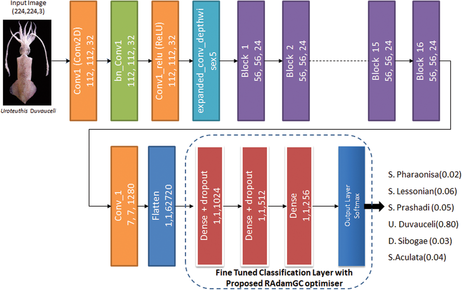
Figure 2: Fine-tunedMobileNetV2 model

2.3.2 Fine Tuned NASNet Mobile Architecture

The brain team of google has created the Neural Architecture Search Network (NASNet), which has two main cell functions; (1) Normal cell and (2) Reduction Cell. NASNet [24] has performed its operations on a small dataset before transferring its block to a larger dataset to achieve a higher mean Average Precision (mAP). The output of NASNet is enhanced by a tweaked drop path called Scheduled drop path for successful regularization. In the first NASNet, the number of cells in the architecture is not pre-determined. Normal and reduction cells are used in particular. The size of the feature map is described by normal cells, and the reduction cell returns the reduced feature map in terms of height and width by a factor of two.

The controlled architecture of NASNet, which is built on a Recurrent Neural Network (RNN), predicts the entire structure of the network based on the two initial hidden states. The Controller Architecture employs an RNN-based LSTM model, with softmax prediction for convolutional cells prediction and recursive construction of network motifs. In NASNet Mobile, the input image size used is 224 × 224. For the transfer learning process, NASNetMobile employs ImageNet pre-trained network weights to classify the cephalopods. The classification layers of the pre-trained NASNet Mobile model are fine-tuned as shown in Fig. 3 for the cephalopod classification task. The model is fine-tuned with three fully connected layers with dropouts, a softmax layer, and an output classification layer to achieve a high categorization rate. The learning rate factor with fully connected layers are increased to accelerate the learning in the new final layers with the proposed optimizer. The performance of the model is evaluated by tweaking higher parameters.

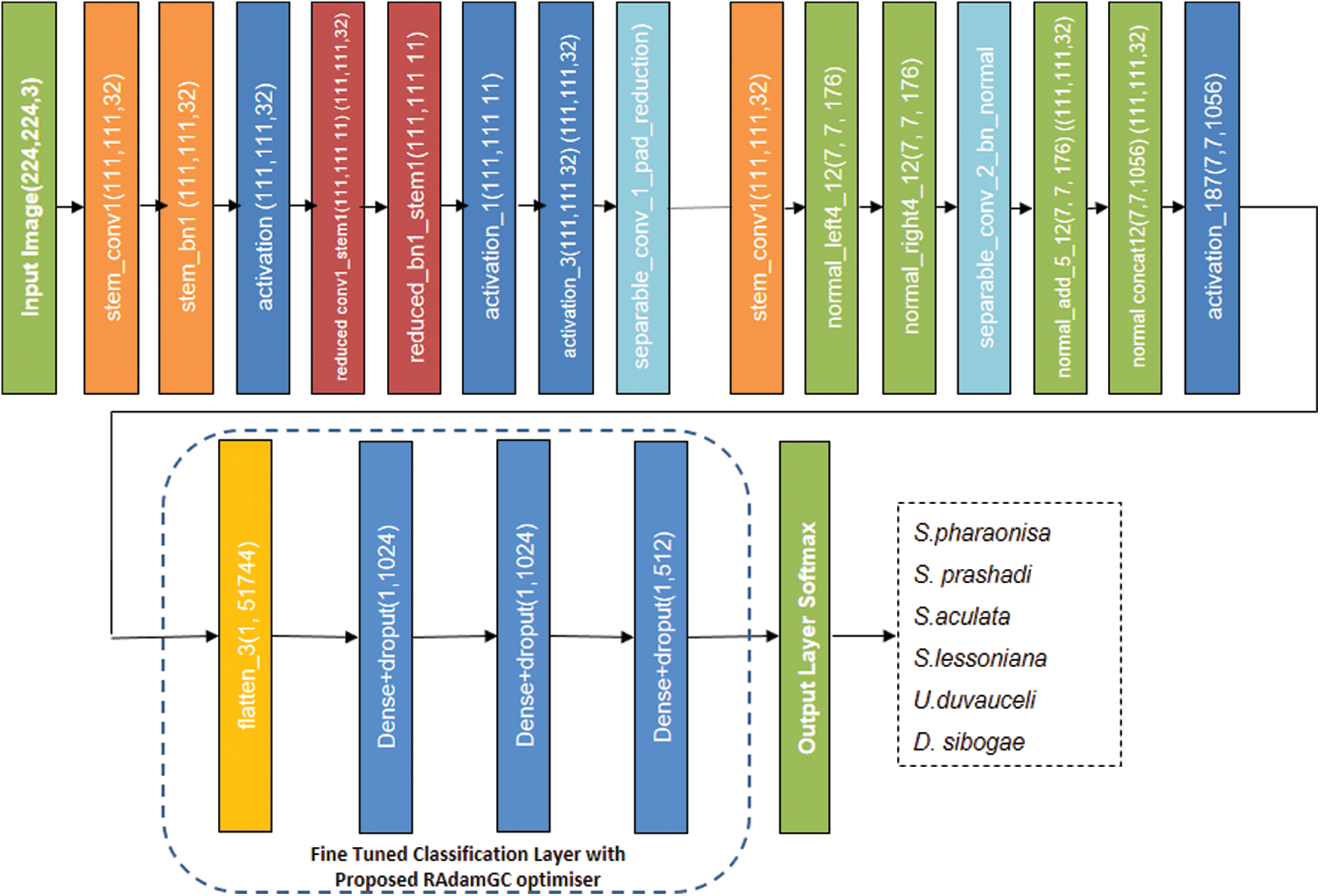
Figure 3: Fine-tuned NASNet Mobile model

2.3.3 Fine Tuned InceptionV3 Architecture

The advent of Inception models inhibits the stacking layer mode, allowing us to expand the depth and width in a new way. Because the variety of modules in an inception model is more complex to design than a Visual Geometry Group (VGG). On the other hand, inception models can be built more extensively and broadly under the same computational budget, resulting in greater accuracy than a VGG. The Inception paradigm has gone through four generations; Inception-V1, Inception-V2, Inception-V3, and Inception-V4. Inception-V2 replaces the 5 × 5 convolutional layers of Inception v1with two 3 × 3 convolutional layers in a row. Asymmetric convolutions are used in Inception-V3 and Inception-V4 to expand the depth, although the former has fewer model parameters. The classification layers of the pre-trained InceptionV3 model have been fine-tuned for our cephalopod classification task. The fully connected layers with dropouts, a softmax layer, and an output classification layer replace the final layers of the model. The learning rate factor with fully connected layers is varied to accelerate the learning in the new final layers. The performance is observed by tweaking the other hyperparameters.

2.3.4 DenseNet201

A feed-forward network, the Dense Convolutional Network (DenseNet), in which each layer is linked to every other layer. Direct connections L(L + 1)/2 are used in this network. All the feature maps of previous levels are used as inputs into each layer, and the feature maps of the layer are being used as inputs in all the following layers. DenseNets have several compelling advantages, including eliminating the vanishing-gradient problem, improved feature propagation, reuse of features, and a considerable reduction in the number of parameters. For Cephalopod classification, DenseNet201 is used. The DenseNet201 is a 201-layer deep CNN. It is a member of the DenseNet family of image classification models.

2.3.5 Xception

Xception is a more advanced variant of the Inception model that independently performs channel-wise and cross-channel convolutions. The primary operator in Xception is a separable convolution, which significantly reduces the parameters of regular convolutions. Xception uses a smaller window (3 × 3) for channel-wise convolution, which is similar to VGG networks. 1 × 1 standard convolutions are performed for cross-channel convolution. Inception models outperform the other types of networks in the classification of accuracy because of the multi-scale processing modules within them.

2.3.6 ResNet50

The ResNet-50 model and aggregation of ResNet models of various depths gained recognition for image classification. ResNet-50 is a residual network of 50 layers that aims to resolve the issue of vanishing gradients in CNN during back-propagation. Increasing the depth of the network can enhance its accuracy if over-fitting is taken into consideration. As the depth of the network rises, the signal needed to modify the weights, which originates from comparing the ground truth and prediction (seen vs. forecasted) at the end of the network, becomes extremely tiny at the early layers. Essentially, it implies that the layers before it is nearly unlearned. The ResNet-50 model relies heavily on the convolution blocks. Multiple filters are applied on these networks to distinguish the images, and the filters are passed over the original image of the strides. The values from the learned filters are multiplied by the values from the images. The outputs of the filters are pooled, thereby down sampling while preserving the essential characteristics.

2.3.7 Proposed Optimization Approach- Rectified Adam with Gradient Centralisation (RAdamGC)

Rectified Adam, often known as Adam, is a stochastic optimizer variation that adds a term to correct the variance of adaptive learning rate. In order to improve the accuracy in cephalopod classification, the optimizer Rectified Adam proposed in [25] is adopted and fine-tuned.

The values of ϕ(.) and ψ(.) , may be changed to provide different optimization techniques, where ϕ(.) indicates how the momentum is determined at time step t and ψ(.) specifies how the adaptive rate of learning is calculated. For example, in the Adam algorithm,

ϕ(g1,⋯,gt)=(1−β1)∑i=1tβ1t−igi1−β1tandψ(g1,⋯,gt)=1−β2t(1−β2)∑i=1tβ2t−igi2 (1)

The function ψ(.) in Eq. (1) is commonly computed as in Eq. (2).

ψ^(g1,⋯,gt)=1−β2ϵ+(1−β2)∑i=1tβ2t−tg12 (2)

In generic adaptive optimisation method, calculation of gradients with respect to stochastic objective at time step t, momentum, adaptive learning rate, updating parameters are given as follows (Eqs. (3)–(6)).

gt←∇θft(θt−1) (3)

mt←ϕt(g1,⋯,gt) (4)

lt←ψt(g1,⋯,gt) (5)

θt←θt−1−αtmtlt (6)

In real-world applications, the Exponential Moving Average (EMA) can be interpreted as a close approximation to the Simple Moving Average (SMA), which is given in Eq. (7).

p((1−β2)∑i=1tβ2t−igi21−β2t)≈p(∑i=1f(t,β2)gt+1−i2f(t,β2)) (7)

where f(t,β2) is the length of SMA, allowing the SMA and the EMA to share the same “center of mass.” In other words, f(t,β2) satisfies the following condition which is given in Eq. (8).

(1−β2)∑i=1tβ2t−i⋅i1−β2t=∑i=1f(t,β2)(t+1−i)f(t,β2) (8)

By solving Eq. (8), we get the Eq. (9) as follows:

f(t,β2)=21−β2−1−2tβ2t1−β2t (9)

For ease of notation, f(t,β2) is marked as ρt . Also, we refer 21−β2−1asρ∞ (maximum length of the approximated SMA), due to the inequality f(t,β2)≤limt→∞⁡f(t,β2)21−β2−1

The rectification term can be calculated as in Eq. (10):

rt=(ρt−4)(ρt−2)ρ∞(ρ∞−4)(ρ∞−2)ρt (10)

Gradient Centralization (GC) is a technique [26] for bringing gradient vectors to a zero mean. GC improves the gradient of the loss function, enhancing the efficiency and consistency of the training process.

It is assumed that the gradient of an FC or convolution layer via propagating backwards is obtained, then, for a weight vector wi whose gradient is ∇wiL(i=1,2,…,N) , the GC operator, denoted by ΦGC , is given in Eq. (11).

ΦGC(∇wiL)=∇wiL−μ∇wiL (11)

where represent the gradient of L w.r.t. the weight matrix W and weight vector wi, respectively.

The GC formula is pretty straight forward. The mean of the weight matrix's column vectors must be computed, and then the mean must be removed from each column vector.

In optimising the cephalopod classification, GC is embedded with RAdam to boost the performance of the network model and to reduce the training time extensively. It is proposed to have an algorithm RAdamGC to raise the performance of the model and save time for training. To embed GC with RAdam, the parameter updates are carried out as shown in Eqs. (12)–(16) and embedded with RAdam algorithm.

gt←∇θft(θt−1) (12)

gt^←∅GC(gt) (13)

mt←β1mt−1+(1−β1)gt^ (14)

vt←β2vt−1+(1−β2)gt^⊙gt^ (15)

mt^←mt(1−β1t) (16)

With the equation, gt^←∅GC(gt) gradient centralisation is applied for calculating the gradients at timestamp t with respect to stochastic objective. Then exponential moving 1st moment mt←β1mt−1+(1−β1)gt^ is calculated with GC. Bias corrected moving average is calculated with mt^←mt/(1−β1t) . In the classification task, the proposed algorithm is utilized using initial values of ρt→7 for MobileNetV2 and ρt→6 for InceptionV3 and NASNet Mobile. For MobileNetV2, InceptionV3, and NASNet Mobile, the initial learning rate is 1e−8, 1e−6, and le−5, respectively.

3  Experimentation and Results

The experiments were carried out in Google Colab Pro, a computational tool that included a Jupyter notebook environment with 25 GB RAM and a GPU interface. Before being applied to pre-trained models, the images were resized to 224 × 224 pixels. Image augmentation was performed while training the model with the Image Data Generator class available in the Keras deep learning neural network library. Initially, the lightweight models namely MobileNetV2, NASNet Mobile, Densenet201, Xception, InceptionV3, ResNet50, were considered for evaluation. Each model was under 100 MB and was considered to be a lightweight model.

3.1 Evaluation of Pre-Trained Models

Adaptive Moment Estimation is a technique for optimizing the gradient descent algorithms. The models were evaluated for the pre-processed dataset. The pre-trained models with a dense layer at their output were trained with an Adam optimizer. Beta one and beta two values were set to values 0.9 and 0.999 correspondingly. The learning rate used with Adam was 0.001. The experiment had used several epochs up to 100. Of the whole cephalopod images, 70% of the total images were used for training, 15%were used for validation, and 15% for testing.

Six different pre-trained models that were considered in the work were evaluated for the classification of accuracy. From the results shown in Fig. 4, it can be observed that InceptionV3 gives the highest accuracy of 82.69%. NASNet Mobile and DenseNet201 have provided an accuracy of 82.05%. The very lightweight model MobileNetV2 has an accuracy value of only 80.77%.

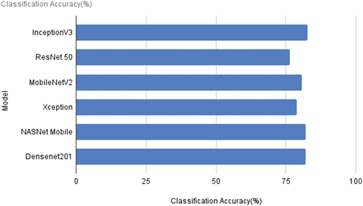
Figure 4: Classification accuracy of the models

Based on the accuracy and size of the models, three are chosen for fine-tuning from the results above. When the outputs of Xception and ResNet 50 are observed, both of them provide less than 80% of accuracy. Despite its 92 MB size, Inception V3 is selected for further fine-tuning to assess the accuracy. Following that, the NASNet Mobile is selected since it is, exceptionally light in weight. Due to its tiny size compared to the other models, MobileNetV2 is also picked for additional fine-tuning.

3.2 Evaluation of Fine Tuned Pre-Trained Models

The evaluation of model is performed by varying dense layers and by employing fine-tuned optimisers to reduce the loss and to improve the performance of the models

3.2.1 Effect on Adding Additional Dense Layers

An improved classification model with dense layers is used to improve the accuracy of classification. Initially, the optimizer Adam is used with the default learning rate. According to the results of the fine-tuned models, there is a significant improvement in the inaccuracy. MobileNetV2 has achieved an accuracy of 84.62%, while the other lightweight model NASNet Mobile has achieved only 84.08%. The classification accuracy of InceptionV3 is 84.61%. Fig. 5 compares the models that have and do not have fine-tuning. Fine-tuning has improved the performance of all models.

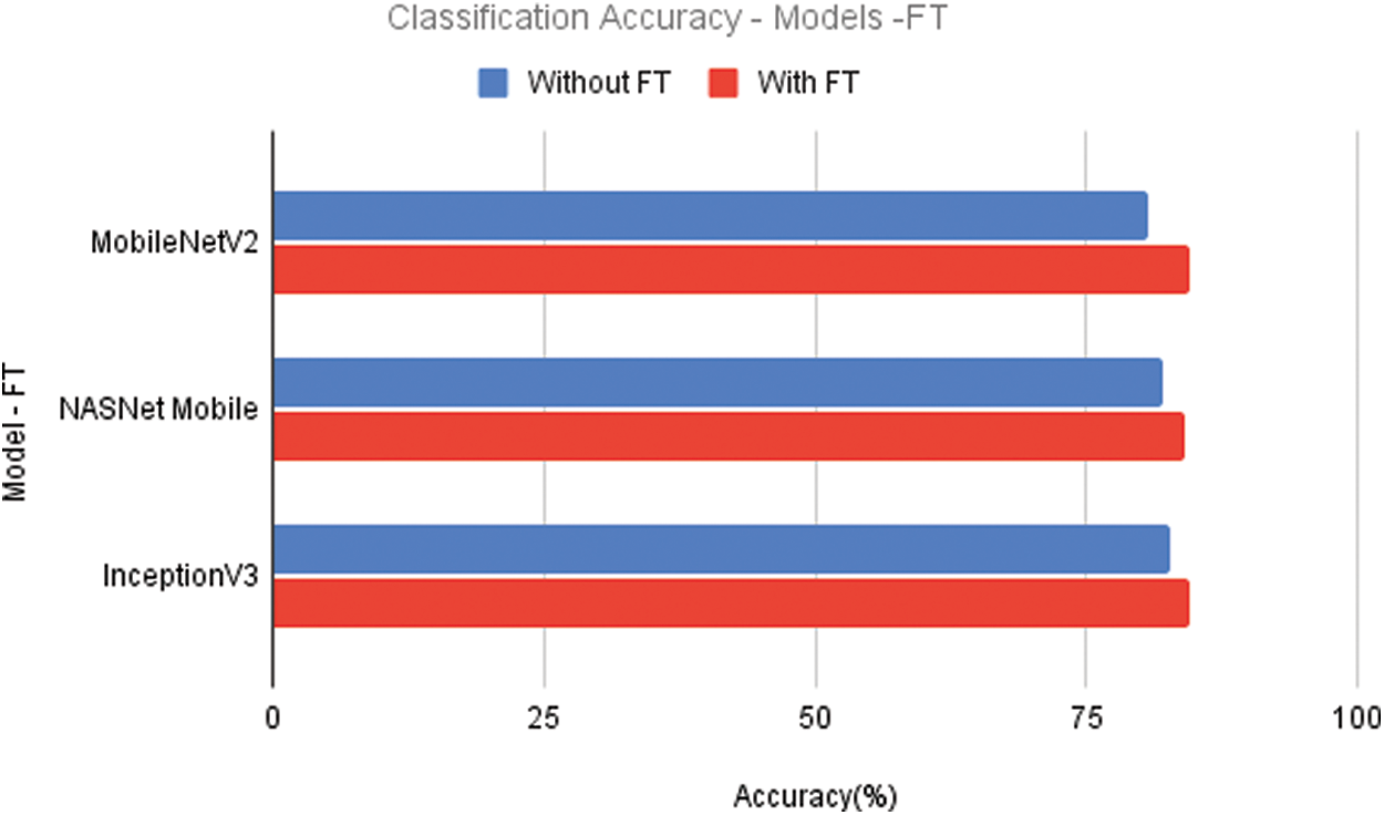
Figure 5: Comparison of models with and without fine tuning (FT)

The performance of MobileNetV2 has significantly improved since the models are fine-tuned. The accuracy of the models NASNET Mobile and InceptionV3 fine-tuned with dense layers have increased by 2%. The accuracy of MobileNetV2 has increased by 4%.

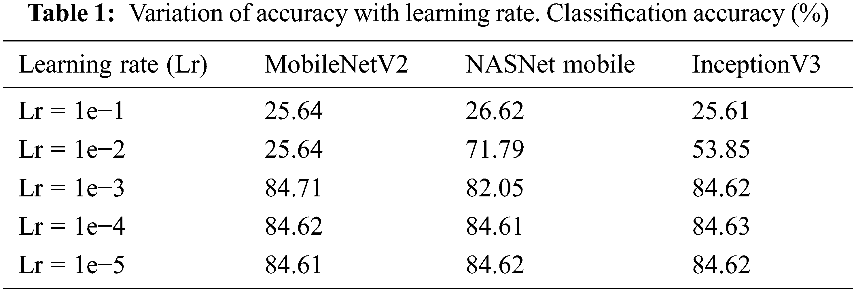
3.2.2 Effect of Learning Rate (Lr)

In an optimization algorithm, the Lr is a tweaking parameter that controls the step size at each iteration while progressing towards a minimum of loss function. A higher learning rate causes the loss function to rise, whereas a slower learning rate causes the loss function to decline progressively.

The best learning rate must be determined to minimize the loss function in the cephalopod classification task. To assess the performance of the model, the models are now trained using learning rates of 1e−1, 1e−2, 1e−3, 1e−4, and 1e−5. Tab. 1 gives the accuracy values when the model is tested with varied learning rates. The MobileNetV2 model performs the best for the Lr of 1e−3. It gives an accuracy of 84.71% with Lr of 1e−3. NASNet Mobile gives the accuracy of 84.62% with the Lr of 1e−5. With the Lr, 1e−4, InceptionV3 gives the accuracy of 84.63%.

3.3 Effect of Optimiser-Improved Rectified Adam

When the approximated SMA length is less than or equal to 4, the variance of adaptive learning rate is intractable, and the adaptive learning rate is inactivated. Otherwise, the variance rectification term is calculated, and the adaptive learning rate is employed to update the parameters. In order to enhance the performance, the fine-tuned models are tested with different values. As shown in Tab. 2, the variation has significant improvement in the performance of the models.

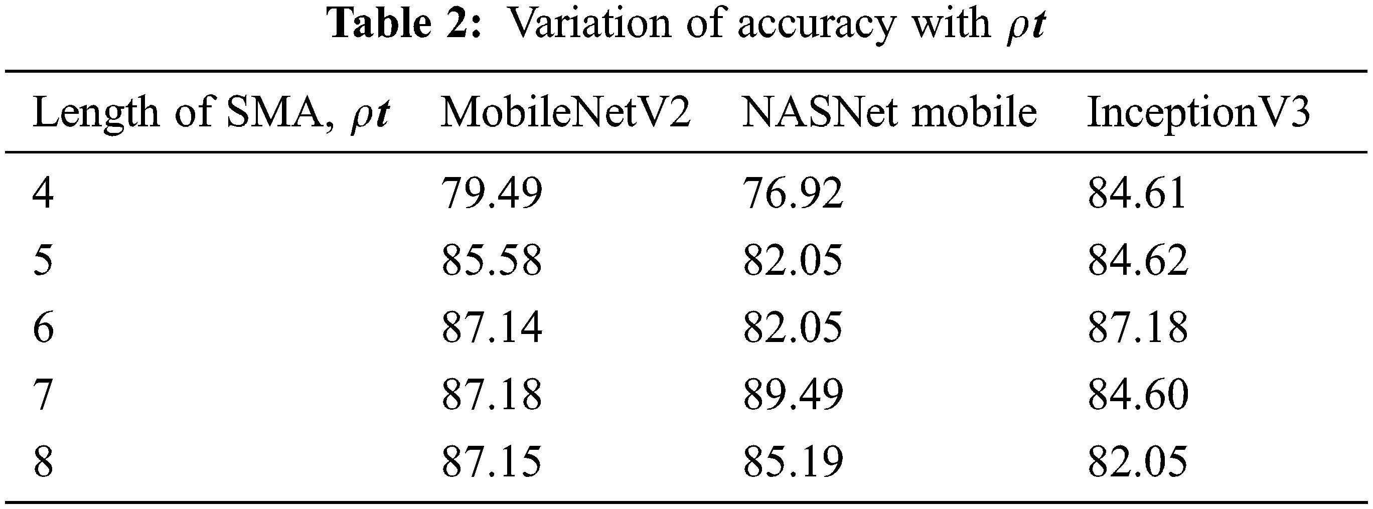
The accuracy of MobileNetV2 is 87.18% with SMA length of 7. NASNet Mobile produces 89.49% for the SMA value of 7. InceptionV3 gives the accuracy of 87.18% with the SMA length of 6.

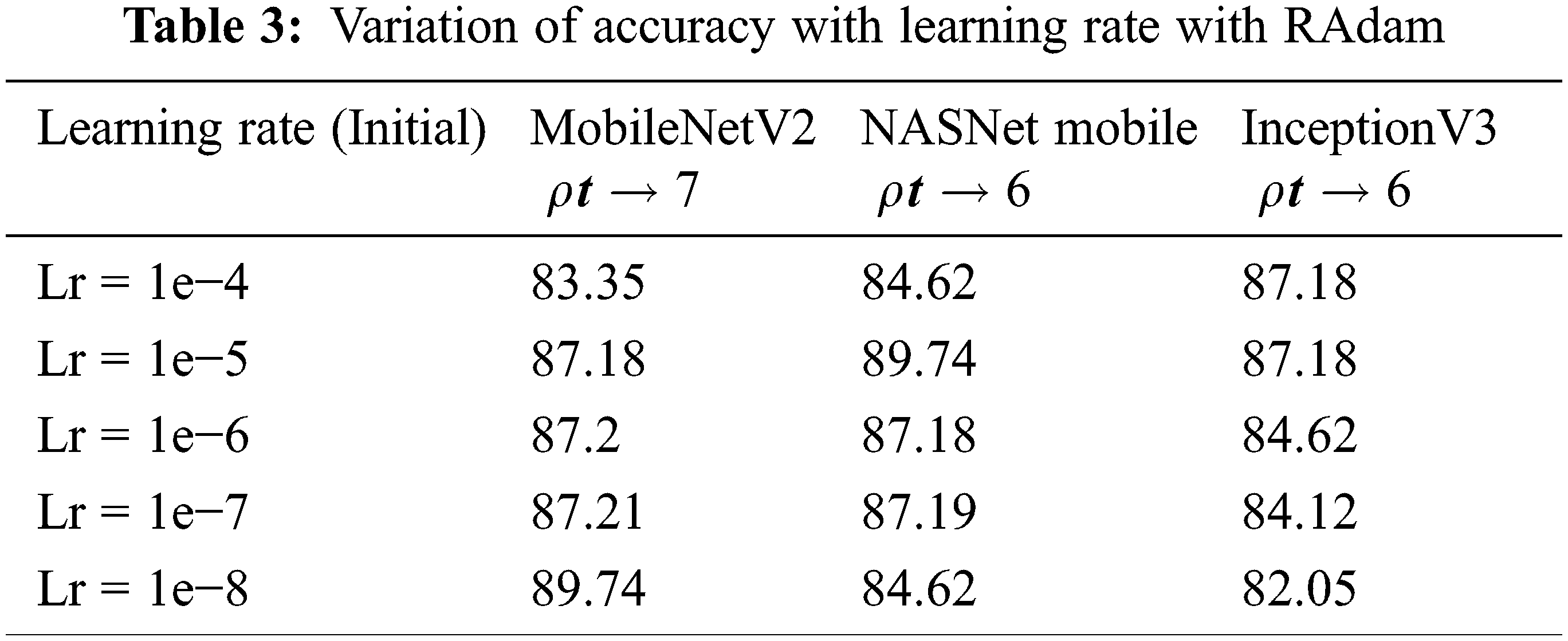
In order to find the optimal learning rate, Learning rate (Lr) is varied from 1e−4 to 1e−8 by setting the optimal values of ρt obtained. MobileNetV2 has attained the maximum accuracy of 89.74% with an Lr of 1e−8, as shown in Tab. 3. The performance of NASNet is increased apparently when compared to the Adam and it also gives the accuracy of 89.74%. InceptionV3 has achieved the accuracy of 87.18% with the Lr of 1e−4 and 1e−5.

The performance measure values of various models for categorizing the species are shown in Tab. 4. The MobileNetV2 Model, which has a precision of 1.00 for four different classes, provides the best results. The accuracy of the Sephia aculeata class is 0.83 with NASNet Mobile and InceptionV3.

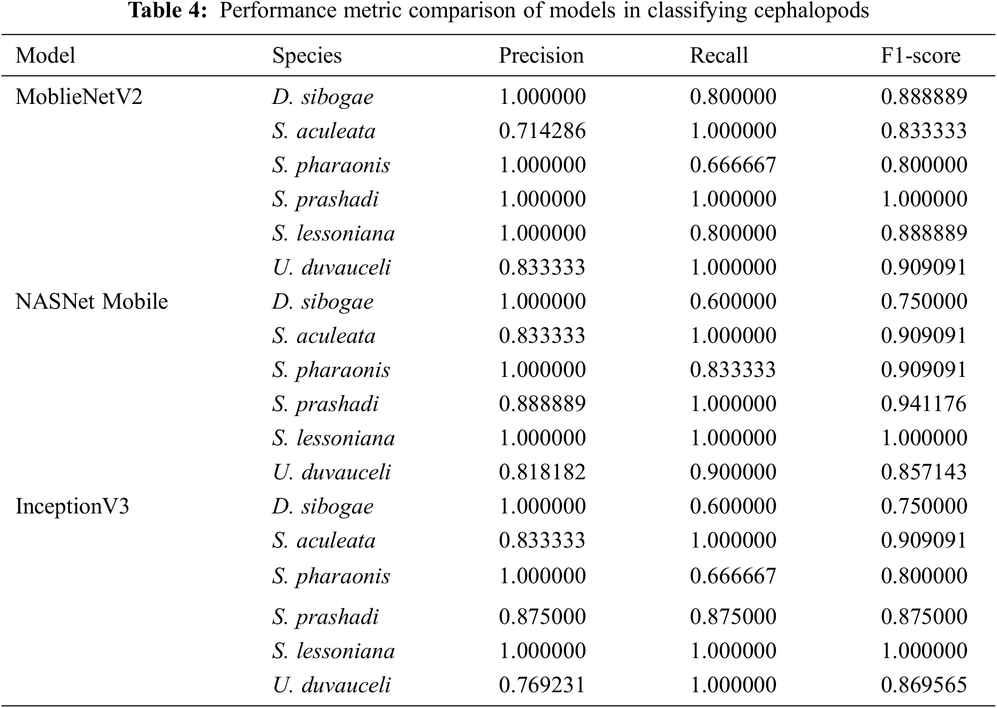
The recall is the measure of the proposed model identifying the cephalopods in a right way. MobileNetV2 gives a reasonable recall rate of 1.00 for the classes S. aculeata, S. Prashadi, & U. duvauceli. In comparison with the other models, NASNet Mobile predicts S. pharaonis in an appropriate manner. MobileNetV2 has a higher recall rate for D. sibogae compared to the other two models.

When compared to the other species, the F1 score shows that the MobileNetV2 model is accurate in classifying S. prashadi, while NASNet Mobile and InceptionV3 accurately categorize S. lessoniana

The performance of various models on a basis of species-by-species is depicted in Fig. 6. MobileNetV2 outperforms in predicting the species S. pharaonis, D. sibogae performs better. S. pharaonis, U. duvauceli, and S. aculata are accurately predicted by NASNet Mobile which outperforms the other models. InceptionV3 predicts S. lessoniana in an accurate way when compared to the other models. When it comes to classifying the other species, it falls short.

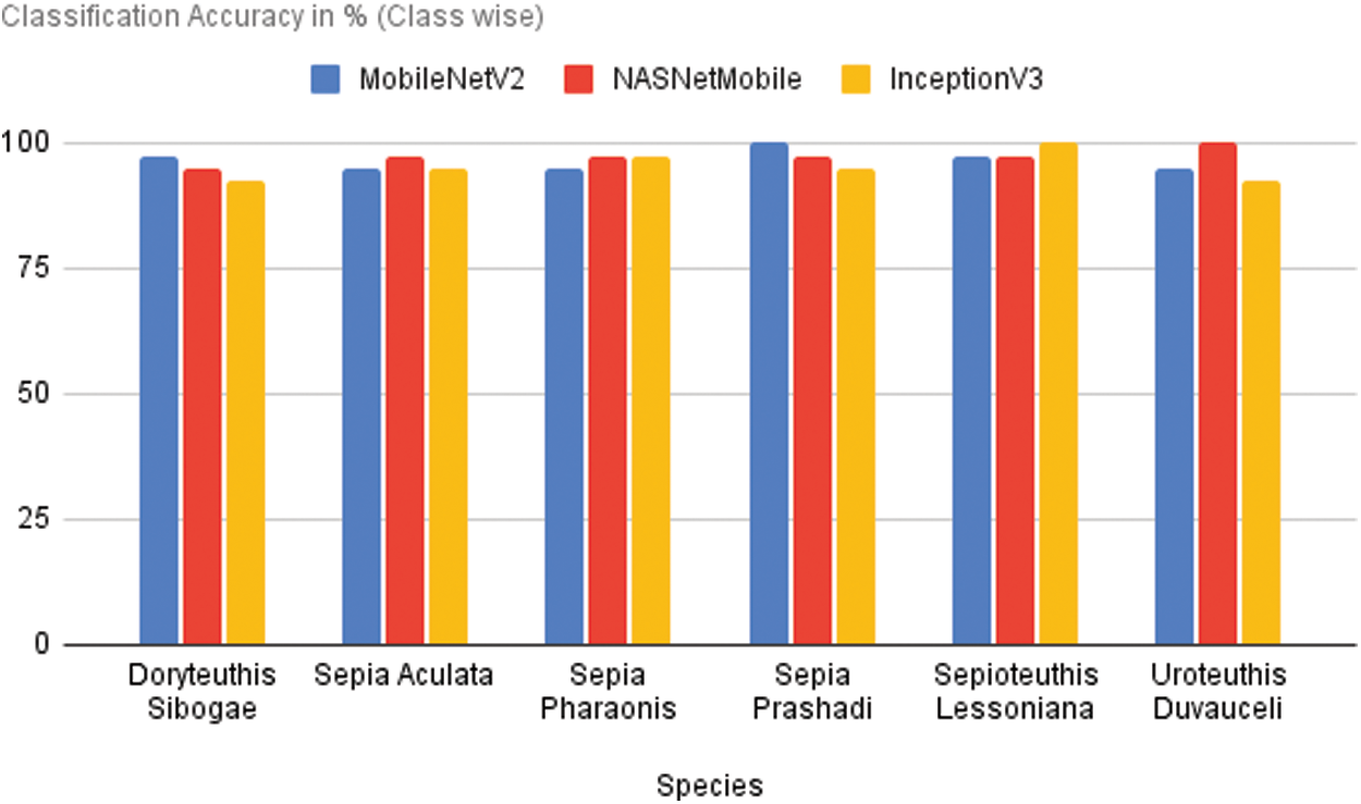
Figure 6: Performance of different models on species wise

The classification accuracy of all models with and without fine-tuning is shown in Fig. 7. After fine-tuning with dense layers and by varying values of parameter change in Rectified Adam, both MobileNetV2 and NASNet Mobile have produced good results.

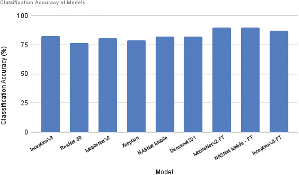
Figure 7: Performance comparison of all models (with and without Fine Tuning)

There is a significant improvement in Inceptionv3 after fine tuning but it is comparatively less when compared to the other fine-tuned models.

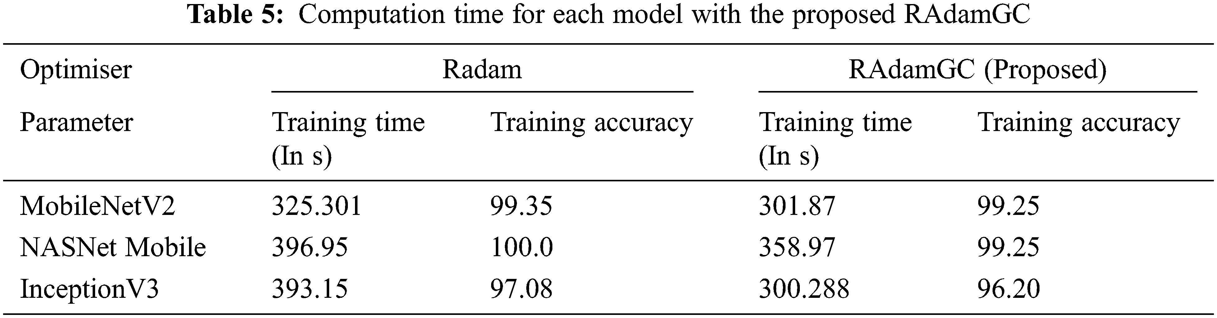
3.4 Computation Time with RAdamGC

The Proposed RAdamGC optimiser is used with the models MobileNetV2, NASNetMobile, InceptionV3.

The training time with the proposed optimizer is significantly reduced, as seen in Tab. 5. MobileNetV2 requires 301.87 s of training time with RAdamGC and 23.43 s of additional training time with Adam. With Adam, NASNet Mobile takes the training time of 396.95 s without GC, but there is a reduction in time of 37.98 s with GC. InceptionV3 requires significantly less training time of 300.288 s with GC, and it is 97.08 s less when compared to Adam without GC. There is a very slight difference in training accuracy with and without GC in cephalopod classification.

4  Discussion

It is evident from the findings that NASNet Mobile, MobileNetV2, and InceptionV3 models had outperformed than the other lightweight models. Fine-tuning of the models with dense layers had given the accuracy of 84.62% with MobileNetV2, 84.08% with NASNet and 84.61% with InceptionV3. The performance of the models was evaluated with Adam by adjusting the learning rates. For learning rates of 1e−3 and 1e−4, the performance of the models was extraordinary. The improved rectified adam was utilized for training to reduce further loss and improve its performance. The models had performed much better for SMA thresholds of 6 and 7. NASNET mobile and MobileNetV2 had produced an accuracy of 89.74% with a learning rate of 1e-8 and 1e-7, respectively. Fine Tuned MobileNetV2 and NASNET Mobile could be utilized to classify cephalopods with extreme certainty. These networks could also be used as an ‘ON DEVICE NETWORK’ for the classification of cephalopods with IoT devices or embedded devices. In order to reduce the training time, gradient centralization was embedded with RAdam. The proposed RAdamGC was applied to evaluate the performance of the model. The findings of the study had indicated that there is a much reduction in the training time with RAdamGC in comparision with all three models.

5  Conclusions

Without the manual and direct observation of cephalopods by marine scientists, the classification of cephalopod is quite a challenging task. This paper has proposed a system to alleviate the manual and the direct process of species classification. The proposed method enables an IoT device or a mobile application to perform the classification tasks by embedding a suitable lightweight pre-trained network. In this paper, six lightweight models are chosen and evaluated. Furthermore, three models are selected based on their performances and fine-tuned to improve the classification rate. As per the evaluation results of the three models, MobileNetV2 and NASNet Mobile have attained a higher degree of accuracy with 89.74%. Because of their light weight, these models are ideal for IoT and mobile devices. An IoT device embedded with such networks can be installed in boats and ships to identify the cephalopods that live beneath the surface of the water. The approach that is used in this study is the first step towards identifying hundreds or thousands of cephalopods. Future investigation is required to expand the range of situations in which the network is adequate for most of the species. In future, the proposed work can not only be developed to categorize the cephalopods into species but also to locate and count them, as well as to estimate their size using images. Detection and segmentation of cephalopods' can also be accomplished using well-known object detection and segmentation techniques.

Funding Statement: The authors received no specific funding for this study.

Conflicts of Interest: The authors declare that they have no conflicts of interest to report regarding the present study.

References

 1.  P. G. Rodhouse, “Role of squid in the southern ocean pelagic ecosystem and the possible consequences of climate change,” Deep Sea Research Part II: Topical Studies in Oceanography, vol. 95, pp. 129–138, 2013. [Google Scholar]

 2.  W. J. Overholtz, L. D. Jacobson and J. S. Link, “An ecosystem approach for assessment advice and biological reference points for the gulf of maine georges bank atlantic herring complex,” North American Journal of Fisheries Management, vol. 28, no. 1, pp. 247–257, 2008. [Google Scholar]

 3.  M. C. Tyrrell, J. S. Link and H. Moustahfid, “The importance of including predation in fish population models: Implications for biological reference points,” Fisheries Research, vol. 108, no. 1, pp. 1–8, 2011. [Google Scholar]

 4.  J. Quinteiro, C. G. Sotelo, H. Rehbein, S. E. Pryde, I. Medina et al., “Use of mtDNA direct polymerase chain reaction (PCR) sequencing and PCR restriction fragment length polymorphism methodologies in species identification of canned tuna,” Journal of Agricultural and Food Chemistry, vol. 46, no. 4, pp. 1662–1669, 1998. [Google Scholar]

 5.  I. M. Mackie, S. E. Pryde, C. GonzalesSotelo, I. Medina, R. PérezMartın et al., “Challenges in the identification of species of canned fish,” Trends in Food Science & Technology, vol. 10, no. 1, pp. 9–14, 1999. [Google Scholar]

 6.  J. Wäldchen and P. Mäder, “Machine learning for image based species identification,” Methods in Ecology and Evolution, vol. 9, no. 11, pp. 2216–2225, 2018. [Google Scholar]

 7.  J. Wäldchen, M. Rzanny, M. Seeland and P. Mäder, “Automated plant species identification—Trends and future directions,” PLOS Computational Biology, vol. 14, no. 4, pp. e1005993, 2018. [Google Scholar]

 8.  F. EmmertStreib, Z. Yang, H. Feng, S. Tripathi and M. Dehmer, “An introductory review of deep learning for prediction models with big data,” Frontiers in Artificial Intelligence, vol. 3, pp. 4, 2020. [Google Scholar]

 9.  S. R. Jena, S. T. George and D. N. Ponraj, “Modeling an effectual multi-section you only look once for enhancing lung cancer prediction,” International Journal of Imaging Systems and Technology, vol. 31, no. 4, pp. 2144–2157, 2021. [Google Scholar]

10. Y. LeCun, Y. Bengio and G. Hinton, “Deep learning,” Nature, vol. 521, no. 7553, pp. 436–444, 2015. [Google Scholar]

11. S. Khan and T. Yairi, “A review on the application of deep learning in system health management,” Mechanical Systems and Signal Processing, vol. 107, no. 2, pp. 241–265, 2018. [Google Scholar]

12. A. Salman, A. Jalal, F. Shafait, A. Mian, M. Shortis et al., “Fish species classification in unconstrained underwater environments based on deep learning,” Limnology and Oceanography: Methods, vol. 14, no. 9, pp. 570–585, 2016. [Google Scholar]

13. S. A. Siddiqui, A. Salman, M. I. Malik, F. Shafait, A. Mian et al., “Automatic fish species classification in underwater videos: Exploiting pre-trained deep neural network models to compensate for limited labelled data,” ICES Journal of Marine Science, vol. 75, no. 1, pp. 374–389, 2018. [Google Scholar]

14. V. Allken, N. O. Handegard, S. Rosen, T. Schreyeck, T. Mahiout et al., “Fish species identification using a convolutional neural network trained on synthetic data,” ICES Journal of Marine Science, vol. 76, no. 1, pp. 342–349, 2019. [Google Scholar]

15. M. Mathur, D. Vasudev, S. Sahoo, D. Jain and N. Goel, “Crosspooled fishnet: Transfer learning based fish species classification model,” Multimedia Tools and Applications, vol. 79, no. 41, pp. 31625–31643, 2019. [Google Scholar]

16. X. Xu, W. Li and Q. Duan, “Transfer learning and SE-ResNet152 networks-based for small-scale unbalanced fish species identification,” Computers and Electronics in Agriculture, vol. 180, pp. 105878, 2021. [Google Scholar]

17. J. A. Jose, C. S. Kumar and S. Sureshkumar, “Tuna classification using super learner ensemble of region based CNN-grouped 2D-LBP models,” Information Processing in Agriculture, vol. 9, no. 1, pp. 68–79, 2021. [Google Scholar]

18. M. A. Iqbal, Z. Wang, Z. A. Ali and S. Riaz, “Automatic fish species classification using deep convolutional neural networks,” Wireless Personal Communications, vol. 116, no. 2, pp. 1043–1053, 2021. [Google Scholar]

19. A. S. Winoto, M. Kristianus and C. Premachandra, “Small and slim deep convolutional neural network for mobile device,” IEEE Access, vol. 8, pp. 125210–125222, 2020. [Google Scholar]

20. X. Liu, Z. Jia, X. Hou, M. Fu, L. Ma et al., “Realtime marine animal images classification by embedded system based on mobilenet and transfer learning,” OCEANS 2019-Marseille, vol. 2019, pp. 1–5, 2019. [Google Scholar]

21. Z. Liu, Y. Cao, Y. Li, X. Xiao, Q. Qiu et al., “Automatic diagnosis of fungal keratitis using data augmentation and image fusion with deep convolutional neural network,” Computer Methods and Programs in Biomedicine, vol. 187, no. 11, pp. 105019, 2020. [Google Scholar]

22. D. M. Montserrat, Q. Lin, J. Allebach and E. J. Delp, “Training object detection and recognition CNN models using data augmentation,” Journal Electronic Imaging, vol. 10, no. 10, pp. 27–36, 2017. [Google Scholar]

23. M. Sandler, A. Howard, M. Zhu, A. Zhmoginov and L. C. Chen, “Mobilenetv2: Inverted residuals and linear bottlenecks,” in Proc. IEEE Conf. on Computer Vision and Pattern Recognition, San Juan, USA, pp. 4510–4520, 2018. [Google Scholar]

24. B. Zoph, V. Vasudevan, J. Shlens and Q. V. Le, “Learning transferable architectures for scalable image recognition,” in Proc. IEEE Conf. on Computer Vision and Pattern Recognition, San Juan, USA, pp. 8697–8710, 2018. [Google Scholar]

25. L. Liu, H. Jiang, P. He, W. Chen, X. Liu, J. Gao, J. Han, “On the variance of the adaptive learning rate and beyond”. arXiv preprint arXiv:1908.03265, 2019 Aug 8. [Google Scholar]

26. H. Yong, J. Huang, X. Hua, L. Zhang, “Gradient centralization: A new optimization technique for deep neural networks,” In European Conference on Computer Vision. pp. 635–652, 2020. [Google Scholar]