B-Spline-Based Curve Fitting to Cam Pitch Curve Using Reinforcement Learning

1  Introduction

Plate cam is a significant part of mechanical design and manufacturing field [1]. It can not only help virtually specify any desirable output function, but also be used to ensure a curved surface to generate the output function of the follower in motion. The polynomial and simple harmonic motion (SHM) expressions with third-order or higher continuity are widely applied for the cam design [2]. As the computer numerical control (CNC) system does not come with a polynomial or SHM interpolation function, it is essential to adopt a computer-aided manufacturing (CAM) tool to discretize the cam profile into several linear segments presented as a sequence of G01 G-codes. Unfortunately, the tool-path code tends to be verbose and the G01 tool path does not go beyond G0 continuity, which may give rise to feed rate and acceleration fluctuation and produce machinery vibration and unexpected slowdowns during the process [3].

To smoothly match the CNC curves, and improve the quality of B-spline tool paths, Min et.al. [4] proposed a method that takes into account the arc-length-based parameter setting, G2 continuity, and the numerical measure. In another study, Jiang put forward a set of approaches for contour error prediction and compensation on the basis of deep learning and reinforcement learning (RL) [5]. Under the chord error constraint, Bi [6] presented a general, fast and robust B-spline fitting scheme for high-speed interpolation of a micro-line tool path. In [7], a progressive and iterative approximation for least squares (LSPIA) method is applied to avoid numerical instability, and lessen chord errors by applying stretching energy terms. All the above studies adopted online or offline optimization approaches to smooth the B-spline tool path locally or globally when the CNC is in operation. Actually, it is preferable to convert the polynomial or SHM expression of the cam into a B-spline expression before CNC machining so that one can directly use the spline interpolation function to operate the plate cam. To this end, this paper concentrates on the B-spline fitting of the plate cam pitch curve.

For a B-spline curve with a fixed degree, it is a complex nonlinear optimization problem to deal with the numbers and positions of knots or control points of the B-spline curve under the error constraints. While fitting the complex heat treatment curves or noise signal curves with multiple data points, the fitting performance is largely impacted by the appropriate numbers and positions of knots [8], and the methods suggested in [9–11], were thus focused on obtaining the numbers and positions of optimized knots, with little discussion on how to obtain these so-called appropriate number and position of data points.

Although one can create a B-spline curve that approximates the pitch curve by placing as many control points as possible, too many control points will lead to lengthy spline parameters, which is almost the same as using a large number of linear segments to approximate the curve. Instead, we intend to create a B-spline curve that meets the error requirements with the smallest possible number of the control points at the right positions. In practical terms, unless enough information about the shape of the original curve can be obtained a priori can one identify the high-quality feature points on the pitch curve [12]. In a nutshell, we can transform the problem of finding the number and position of control points into the problem of finding the number and position of data points on the pitch curve, and use these data points to determine the control points needed to construct the B-spline curve.

In light of the path planning of the unmanned surface vehicle (USV) [13], we shall be able to obtain the relevant data points for the construction of the B-spline curve. In this case, a pitch curve is treated as an ideal path, and an RL algorithm is applied to find an optimal policy that obtains the appropriate number and position of the data points on the ideal path (i.e. the pitch curve). When the actions set is discrete and the number of states set is limited, a Q-learning algorithm can be adopted to find the rough position of the probe point [14]. Similarly, it is possible to use the visualization table of Q-learning to obtain the optimum data points from the pitch curve. Note that accurately estimating the number and position of data points of an unknown curve that can fit a B-spline is mathematically infeasible. Correspondingly, the dimensions of the Q-table built from the numbers and positions of data points should be discrete in nature, and the searching process of the data points should be made model-free. As the framework of deep Q-network (DQN) is basically the same as that of Q-learning, and DQN adopts a neural network to replace the Q-table in Q-learning, DQN is suitable for model-free control problems with discrete variables. Furthermore, the double deep Q-network (DDQN) algorithm with model-free techniques is found to enhance the robustness of curve matching than supervised machine learning algorithms [15]. Compared with the advanced actor-critic (A2C) algorithm of on-policy, the proximal policy optimization (PPO) algorithm of off-policy and the deep deterministic policy gradient (DDPG) algorithm applicable to continuous and high dimensional action space, DDQN algorithm has a simple framework, fast convergence speed, and the ability to deal with the optimal solution of discrete variables under uncertain dimensions. In simple terms, the DDQN algorithm is more suitable for obtaining the optimal policy through the maximum Q-value, and it is thus adopted as the B-spline fitting algorithm of the pitch curve, as proposed in this paper.

In this paper, we propose a DDQN algorithm with data points traceability to cope with the B-spline fitting of the pitch curve. We take the pitch curve expression as the system environment of RL (see Section 2.1), and the agent applies the actions set A which covers a 360-degree circle to search for interpolation points (see Section 2.2). We then use these interpolation points as the data points on the B-spline curve, and define column vector S which is composed of all the data points’ coordinates, the number of data points and the termination criterion as the current state of the agent (see Section 2.3). Meanwhile, a memory area Ttrack is applied to store the trajectory of data points obtained by every episode iteration for the inverse calculation of B-spline knot vectors and control points. Section 2.4 studies the reward function which is the key part in an RL, and designs single-objective and double-objective reward functions to reduce the radial error of spline fitting. In Section 2.5, we design a neural network for DDQN algorithm, and use a small batch of training sets to train the initial network of DDQN. At the end of Section 2.5, we summarize the detailed procedure of the algorithm put forth in this paper. In Section 3, we select the 5th degree polynomial rise function of a cam for B-spline fitting test. Through the iterative calculation, the control objective of constructing a B-spline curve satisfying the fitting error with a small number of data points is realized. Finally, Section 4 summarizes the paper.

2  Modeling and Training Using RL

2.1 Environment Build

2.1.1 Pitch Curve Expression

To find the data points on the pitch curve, the pitch curve expression is inputted to the RL environment. Let H(φ) and S(φ) represent the displacements of the follower under respective polynomial and SHM expressions, where φ is the cam shaft angle. The n-degree polynomial or SHM function expression of the rise or fall segments adopted by conventional pitch curve is given by

H(φ)=D0+D1φ+D2φ2+⋯+Dnφn (1)

S(φ)=D0+D1cos⁡(D2φ) (2)

The geometry of plate cam is shown in Fig. 1. Here, φ falls into the range of start angle φ0 and end angle φe .The polynomial coefficients Dn can be obtained by the boundary conditions, and the SHM coefficients Dn can be obtained by adopting the laws of SHM and cycloidal motion.

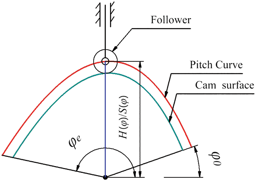
Figure 1: Geometry of plate cam

2.1.2 B-spline Curve Expression

The expression of the B-spline curve is simple and has a favorable local modification. The local shape of the curve can be modified by changing the position of the control points, which meets the fitting requirements of the pitch curve. B-spline curve expression B(u) with parameter u as its variable and its basis function Ni,p(u) are:

B(u)=∑i=0n⁡Ni,p(u)diu∈[0,1] (3)

{Ni,p(u)=u−UiUi+p−UiNi,p−1(u)+Ui+p+1−uUi+p+1−Ui+1Ni+1,p−1(u)Ni,0(u)={1ui≤u<ui+10otherwiseset00=0 (4)

In Eqs. (3) and (4), Ni,p(u) is the basis function, di is the control point, Ui is the knot and U is the knot vector consisting of all the knots. The parameters of B-spline curve are selected as follows:

Number of knots: m+1 ;

Knot vector: U=(U0,U1,⋯,Um) ;

B-spline degree: p = 3;

The number of basis functions Ni,p(u) and control points Pcon : n+1 ;

The number of data points Pin : n−1 .

2.1.3 B-Spline Curve Expression as the Inverse of B-spline Knot Vector and Control Points

To ensure that the B-spline curve and the adjacent curve are G1 continuous at the joint points, the first and last data points on B-spline curve are included as the first and last points on the pitch curve. Next, the clamp property of B-spline is applied to make the positions of the first and last control points coincide with the positions of first and last data points. Correspondingly, the value of the first p+1 knots is set to be 0, and the value of the last p+1 knots is 1. In accordance with the property of B-spline, i.e., m=n+p+1 , the number of interior knots is: m+1−2(p+1)=m−2p−1=n+p+1−2p−1=n−p . The knot vector U can be written as:

U=[0…0⏟p+1Up+1…Um−p−1⏟n−11…1⏟p+1] (5)

The non-uniform interior knots Up+1⋯Um−p−1 are calculated with reference to accumulative chord length method given in Eq. (6) through Eq. (8).

lj=|Pj+1Pj|j=0,1…n−3 (6)

L=∑j=0n−3⁡lj (7)

Ui+1=Ui+li−p−1L(i=p+1,⋯,n+p−3) (8)

Here, Pj is the data point, lj is the chord, and L is the total length of accumulative chord.

After the knot vector is determined, the control points of the B-spline can be solved by applying Eqs. (9) and (10) [16]:

{d0=P0[1g2b2c2⋯gn−2⋯bn−2cn−21][d1d2.dn−2dn−1]=[D1D2.Dn−2Dn−1]dn=Pn−2 (9)

{ Δi=Ui+1−Ui   (i=0,⋯,m−1)gi=(Δi+2)2Δi+Δi+1+Δi+2bi=Δi+2(Δi+Δi+1)Δi+Δi+1+Δi+2+Δi+1(Δi+2+Δi+3)Δi+1+Δi+2+Δi+3ci=(Δi+1)2Δi+1+Δi+2+Δi+3T1=P0−Δ33P0′Dn−1=Pn−2−Δn+13Pn−2′Di=(Δi+1+Δi+2)Pi−1   (i=2,⋯,n−2)}(10)

Here, d0⋯dn are the control points. P0′ and Pn−2′ is the tangent vector of the first and last data point, respectively, which ensures that the B-spline curve meets G1 continuity at the joint points.

In the next, we will show how to use the RL method to search for the data points with appropriate numbers and positions.

2.2 Action Modeling

2.2.1 The Set of Actions

One iteration of RL is shown in Fig. 2. Here the agent starts from the initial point P0 of the pitch curve, and adopts action at to seek the data points in the counter-clockwise direction.

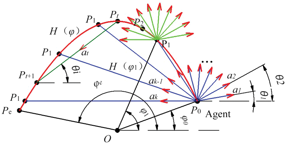
Figure 2: Actions of agent

In Fig. 2, We define the t-th action at of the agent as the linear motion at an angle θi with respect to the horizontal line. We divide (0, π] into k segments, and define the actions set A as:

A=(a1,a2⋯ak−1,ak)=(θ1,θ2⋯θk−1,θk)=(πk,2πk⋯(k−1)πk,π) (11)

Here, θi is the angle between the search line and the horizontal line when the agent applies action at to seek the data points. The agent may seek the data points along or opposite to the direction of the arrow in Fig. 2. Hence, the actions set A ensures that the search range of agent is [0,2π]. The larger the value of k in Eq. (11) is, the smaller the angle division value between adjacent actions is, and the more data points the agent can obtain. In a simple term, we can adjust the maximum number of data points obtained by the agent by varying the value of k .

2.2.2 Solving Data Points Using the Actions Set

We assume that in an iterative calculation, the agent selects an action at to perform a linear motion from the current data point Pt in Fig. 2. If the straight line and the pitch curve have an intersection point Pt+1 , the agent updates the Pt+1 to the current data point. Eq. (12) is established by adopting the coordinates of points Pt and Pt+1 and the slope of the straight line connecting the two points. After replacing coordinates of the data point in Eq. (12) with the projection correlation between the cam stroke and the cam shaft angle in Eqs. (13) and (12) only contains parameters φ that is still unknown. Next, the cam shaft angle and stroke corresponding to the current data point can be dealt with from the deformed Eq. (12), and the coordinate of the current data point Pt+1 will be figured out by substituting φt+1 and H(φt+1) into Eq. (13).

Yt+1−Yt=tan⁡(i ∗180∘k)(Xt+1−Xt) (12)

{Xt+1=H(φt+1)cos⁡(φt+1−φ0)Yt+1=H(φt+1)sin⁡(φt+1−φ0)φϵ[φ0,φe] (13)

The two nonlinear equations, Eqs. (12) and (13), are solved with the agent applying action at from actions set A to find intersection Pt+1 and taking it as the current data point. The solution process requires numerical iteration, and the following points shall be noted in the solution process:

(1) The cam shaft angle φ should locate in the range [φ0,φe] , and the data points exceeding this range shall be removed. Next set Pt+1=Pt , and terminate the search process;

(2) When the equations have no solution, set Pt+1=Pt , and then terminate the search process;

(3) When the updated data point Pt+1 is very close to the end point Pe of the pitch curve, the search process terminates;

(4) When the action at obtains the intersection point Pt+1 as exhibited in Fig. 3, since this type of intersection point does not conform to counter-clockwise direction, taking this type of intersection point as a data point will result in a singular structure of the B-spline curve. As a result, we specify that when OPt+1¯<OPt¯ , action at is an invalid action that cannot find a new data point. We thus set Pt+1=Pt , and end the search process.

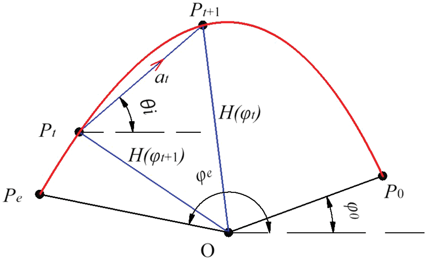
Figure 3: Intersection point that does not conform to counterclockwise direction

2.2.3 Greedy Strategy

Agent adopts a greedy strategy to select the action at in the current state from the actions set A . We define the greedy strategy πg as:

πg(at|S)={1Nnow0.2at=random(A)1−1Nnow0.2at=argmaxQ(S,ai)aiεA (14)

Here, Nnow is the current sequence number during RL iterative calculation. For instance, when Nnow=300,1Nnow0.2=0.3196 , the agent is in the exploration stage, and has a high probability to conduct random exploration. When Nnow=18000 , 1Nnow0.2=0.1409 , the agent is at the end of the iteration, and has a small probability to select actions other than the maximum Q-value.

2.3 Current State Feature Model Build

2.3.1 The Set of States

When the agent adopts the actions defined in Section 2.2 to explore the environment defined in Section 2.1, it should obtain as much current information as possible. We define the set of all states S as:

S=[xyfe]T (15)

Here, x , y are the coordinates of the current data point, and f is adopted to record the number of data points in the current state of the agent. When a new data point is determined from the next state S′ , we set f′ = f+1 . Next, the agent updates the current state and continues to search the next data point; otherwise, we set f′=f , and terminate the state update. e in Eq. 15 is the termination criterion needed to check whether the current data point is close enough to the end point of pitch curve. From Fig. 2, one can see that e is calculated as below:

e={1ifPeO¯−PtO¯<0.50ifPeO¯−PtO¯>0.5 (16)

2.3.2 The Traceback of Data Points

Since the state vector S records the current state, when e=1 , the coordinates of all the data points obtained by the agent before the terminal state need to be obtained to find out the knot vector and the control points. In each iteration, since the number of actions t in each episode is the same as the number of data points f in the current state vector St , the state vector St in Eq. (17) can be encoded using the parameter t or f and mapped to Ttq , as given in Eq. (17).

Ttq=[xtytftetq]T (17)

In Eq. (17), Ttq is adopted to store the state vector St of the f -th acquisition data point in the q -th episode iteration. We use a memory Ttrack to store the trajectories of all completed sequences Ttq for the agent to be able to trace back all the calculated data points.

Due to the mapping correlation between the state vector S and the vector Ttq , each sample can be recorded as (St,at,Rt,St+1,q) during the experience replay of the DDQN algorithm. Fig. 4 shows the traceback process to with the help of memory Ttrack to find all the data points obtained by the agent in the q -th episode at terminal state ( et+1=1 ).

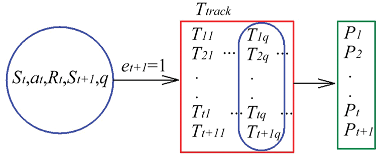
Figure 4: Traceback of the data points through memory Ttrack

2.4 Reward Method

2.4.1 Reward Function for Obtaining the Maximum Number of Data Points

The reward function is of paramount importance to whether or not the agent can learn effective knowledge from the environment and evolve correctly. Regardless whether it is designed as single objective or multi-objective [17], a reward function must meet its control objectives to achieve an expected convergence effect [18]. The control objective in this paper is to construct a spline curve satisfying the fitting error with fewer data points. When the value of k in Eq. (11) is fixed, the angle division value between consecutive actions is unchanged. Although there are many possible combinations for the data point sequences that the agent may obtain, there is at least one combination that can obtain the maximum number of data points. In this case, the fitted B-spline curve is closest to the pitch curve. In order to find the maximum number of data points under a fixed angle division, the reward function R1 is given as:

R1={−10iff1=00if{f1=1ft+1−ft=010if{f1=1ft+1−ft=1 (18)

The reward function defined by Eq. (18) indicates that:

(1) If the agent fails to find the first data point, it will be given a penalty −10 which is the same order of magnitude as the reward value. The larger penalty will encourage the agent to find the first data point in the exploration to speed up the RL algorithm assurance that the agent finds the data points effectively;

(2) If the agent finds the data point after the first action, but cannot find the data point in its current action, it will be rewarded with 0;

(3) When the agent finds the data point after the first action and also finds the new data point in current action, it will be given 10 rewards to encourage the agent to obtain as many data points as possible.

The DDQN algorithm using R1 as the reward function will obtain the following convergence effects after a multitude of iterative calculations: The agent starts from the initial point P0 of the pitch curve, and employs the trained neural network to determine if the action a1∗ can obtain the maximum Q-value in the actions set A in the current state S0 . Thus, the first data point P1 can be determined, and the current state is updated to S1 . Next, the agent continues to use the trained neural network to check the action a2∗ that obtains the maximum Q-value in the actions set A in the S1 state, and determines the second data point P2 . After that, the agent repeats the above operations until the current data point approaches the end point Pe of the pitch curve. The above process is actually a generalized policy iteration (GPI) process using the maximum Q-value. The sequence of actions (a0∗,a1∗…an∗) together constitutes an optimal policy π1∗ using R1 as the reward function. The Bellman Equation for calculating the Q-value is expressed as:

Q(St,at)=E[Rt+γQ(St+1,at+1)] (19)

where γ∈[0,1] is the discount factor, and E[.] is the expectation operation. In this case, Q-value is the mathematical expectation of the algebraic sum of the current reward and the discounted Q-value of the subsequent state. Hence, π1∗ is a global optimal policy, which ensures that the optimal action ai∗ applied by each state transition of the agent is the action that can obtain the largest number of data points in the actions set A in the future. The maximum number of data points thus obtained will ensure the minimum fitting error.

2.4.2 Reward Function for Adjusting the Position of Data Points

Although the reward function R1 can encourage the agent to decrease the fitting error by increasing the number of data points, the only reward R1 determines that the Q-value does not contain the data for calculating the fitting error. When there are many sets of action sequences that can find the same number of data points, the agent is unable to identify which set of action sequence really gives the smallest fitting error. As a result, we need to ameliorate the reward function R1 .

If the eccentricity ε of the cam follower is zero, the polar radius ρ formed by connecting a straight line between the rotation center of the cam and any point on the pitch curve equal to the displacement of the follower, i.e. ρ=H(φ) . If the eccentricity of the cam follower is not zero, the polar radius is ρ=ϵ2+H(φ) . As a result, one can use the length value of the polar radius to describe the motion law of the cam follower, and the error of the polar radius can reflect the displacement error of the cam follower. In the plate cam with non-offset follower, we choose the radial error to study the fitting effect of B-spline curve, and use it to construct the new reward function R2 .

We replace the parameter u in Eqs. (3) and (4) as φ−φ0φe−φ0 to convert B(u) into B(φ) . Next, we define a function F(φ) shown in Eq. (20) as the cumulative radial error of pitch curve H(φ) and spline curve B(φ) , when e=1 .

F(φ)=∑j=1N⁡|H(φj)−B(φj)x2+B(φj)y2| (20)

where B(φj)x2+B(φj)y2 is the polar radius of B-spline when the camshaft angle is φj , H(φj) is the polar radius of the pitch curve at the same angular φj , and N is the number of discrete sampling points on two curves, and its value is set to be 1000. For smaller F(φ) , the spline curve is closer to the pitch curve, and the agent should get more positive rewards. Thus, we include F(φ) to be the denominator of the new reward function R2 . In order to quantify the value R2 and make it match the output Q-value of the neural network when there is just R1 , to avoid the value of R2 being ignored or excessively amplified, a weight coefficient λ is introduced to define reward function R2 as below:

R2={λN/F(φ)ife=10ife=0 (21)

After several experiments, the value of λ is set to be 10.

2.5 The Neural Network of Agent

2.5.1 Neural Network Modeling

Since the number of discrete actions of an agent is limited, it is appropriate to choose an artificial neural network (ANN) with a simple structure. Following the method to setting the number of hidden layers in [19] and testing several dissimilar types of network structures and layers, we select the backward propagation ANN that has an input layer, an output layer, and two hidden layers, as depicted in Fig. 5. The 5 inputs [xtytftetID(at)]T are composed of the current state vector St and the sequence number ID(at) of the action at . The output layer is the value of Q(St,at) . The sizes of the two hidden layers are set to be 20, which can meet the Q-value calculation for 1000 states or more.

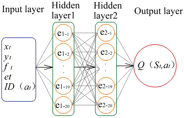
Figure 5: The artificial neural network model

2.5.2 Neural Network Initialization

The initial value of neural network remarkably affects the control performance and training convergence speed [20,21]. At the initial stage of agent searching the data points, if the Q-value estimated by the initial neural network is far from the ideal Q-value, the RL algorithm needs more samples and longer training time to converge.

After several experiments, we find that for constrained input and output variables of the initial neural network, there is no noticeable correlation between them, the convergence speed of the algorithm can be accelerated. Correspondingly, we apply only a small batch of training set to tune the initial parameters of the neural network. In reference to Fig. 5, we define the input and output value range of the training set as:

{xtrain∈[H(φ0)cos⁡φ0,H(φe)cos⁡φe]ytrain∈[H(φ0)sin⁡φ0,H(φe)sin⁡φe]ftrain∈[0,20]etrain=0or1ID(at)train∈[1,k]Qtrain∈[0,0.01] (22)

Here, ftrain,etrain,ID(at)train are integers. xtrain and ytrain are the coordinates of any random point on the pitch curve. ftrain is a guessed number of data points in current state. etrain is the termination flag. ID(at)train is the random sequence number of the action at . Qtrain is the output value of training set, and its interval is [0,0.01] . In order to randomize the training set, a random number v within the range of [0,1] is utilized to define the value of training set as:

{xtrain=H[v(φe−φ0)]cos⁡[φ0+(φe−φ0)v]ytrain=H[v(φe−φ0)]sin⁡[φ0+(φe−φ0)v]ftrain=random[0,20]etrain={0if|H(v)−H(1)|>0.51if|H(u)−H(1)|<0.5ID(at)train=random[1,k]Qtrain=0.01v(23)

We replace xt , yt , ft , et , ID(at) and Q(St,at) in Fig. 5 with xtrain , ytrain , ftrain , etrain , ID(at)train and Qtrain in the training set, respectively, so as to train the initial neural network for the DDQN algorithm. Since the output Q-values of the training samples are randomly spread over the range of [0,0.01] , they are much smaller than the rewards R1 and R2 . As a result, when the DDQN algorithm employs the initial neural network and regards it as the predicted network and the target network, the estimation of Q-value is noticeably affected by the rewards R1 and R1 at the initial stage of iterative calculation, and the agent can converge towards the ideal result at a faster speed.

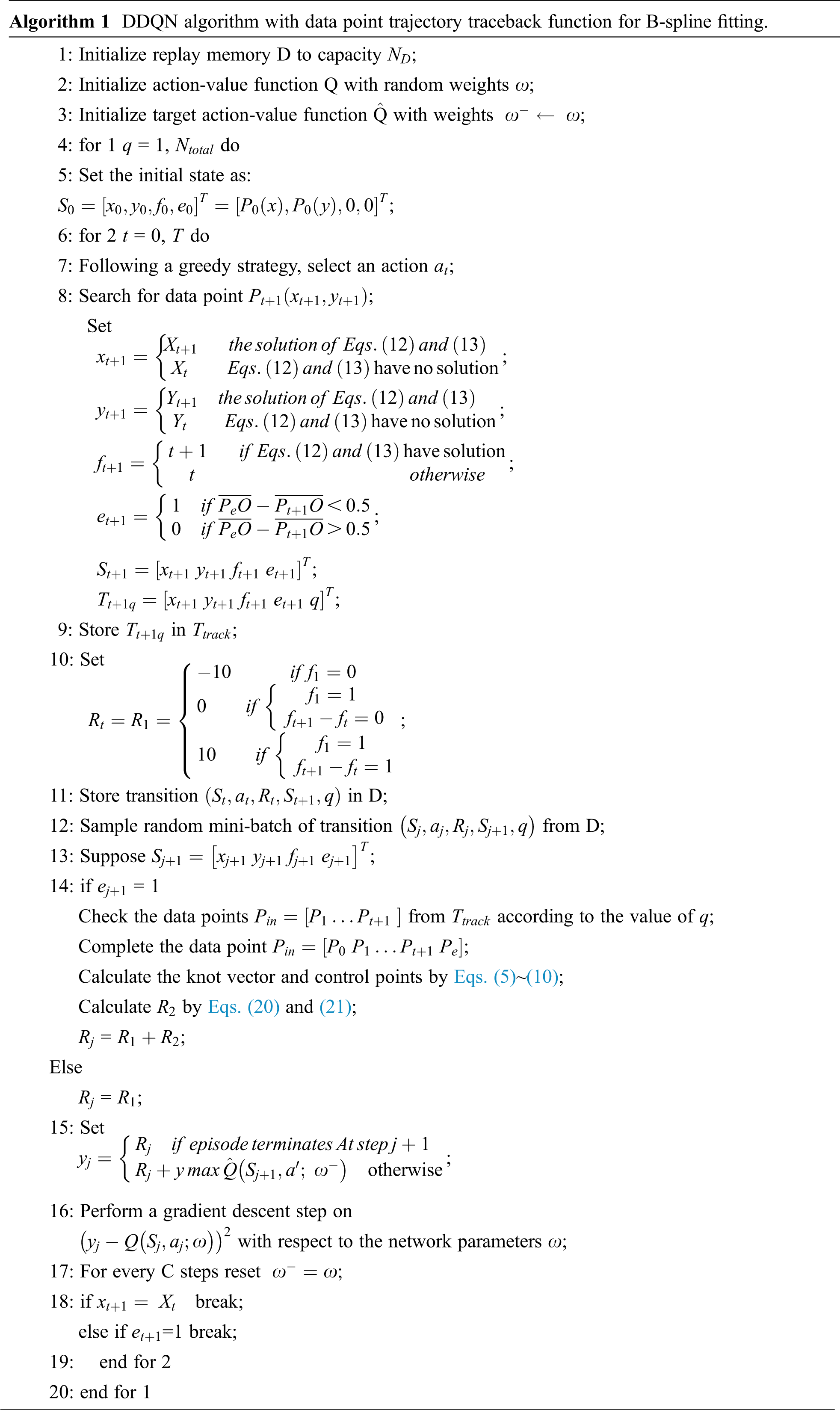
In summary, the DDQN algorithm with data points trajectory traceback function put forward in this paper is detailed in Algorithm 1.

3  Experiment Results

3.1 R1 Reward

We select the 5th degree polynomial rise function of a plate cam as the experiment curve of B-spline fitting. The basic parameters of the cam are: base circle radius rb=17mm , total rise H=10mm , eccentricity of cam-follower ϵ=0 , start angle φ0=0∘ , end angle φe=160∘ , the tangent vectors of the first and last data point are P0′=(0,1) and Pe′=(−0.9397,0.3424) .

And the other boundary conditions of the cam are:

{dHdφ|φ=φ0=0dHdφ|φ=φs=0d2Hdφ2|φ=φ0=0d2Hdφ2|φ=φs=0 (24)

By substituting the basic parameters and boundary conditions of the cam into Eq. (1), the pitch curve H(φ) can be solved as:

H(φ)=17+100(98πφ−1)3−150(98πφ−1)4+60(98πφ−1)5 (25)

The rise segment of pitch curve is shown in Fig. 6.

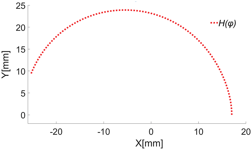
Figure 6: The pitch curve of the plate cam of the rise segment

The actions set A is established by applying the adjacent action angle division of 3°, i.e., k=60 . The maximum number T of data points in Algorithm 1 is 20. The discount factor γ =0.9. The number of neural network initialization training samples is 400, and the online neural network training set contains 400 samples. The target neural network update frequency is 1200. The memory D capacity for storing mini-batch of transition (St,at,Rt,St+1,q) is 400. The memory Ttrack capacity for storing all complete sequences Ttq is the same with the total number of RL iterative calculations Ntotal , both of which are set to be 20,000.

When R1 is utilized as the sole reward function, the 14th step of Algorithm 1 is no longer needed. The number of data points obtained in each episode is shown in Fig. 7. In the first 10000 episodes shown in Fig. 7, the agent can obtain 6 data points as the maximum. Since 14000-th episode, the agent can obtain more than 8 data points. At the 19870-th episode, the agent obtains the 12 data points, which is the largest number in this experiment. As demonstrated by the iterative calculation process, the Algorithm 1 can train an ideal neural network to guide the agent to obtain more data points as the interaction progresses.

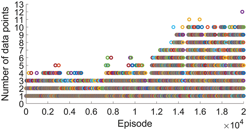
Figure 7: The number of data points obtained in each episode

The relationships between the sequence numbers of all actions and the predicted values Q(S,A) of the neural network during the first four state transitions are plotted in Fig. 8. Table 1 tabulates the maximum output values Q(S,A) in Fig. 8 and the sequence numbers of optimal action ID(a∗) , the coordinates of the data points obtained by applying optimal actions a∗ and the maximum values Q(S,A)L .

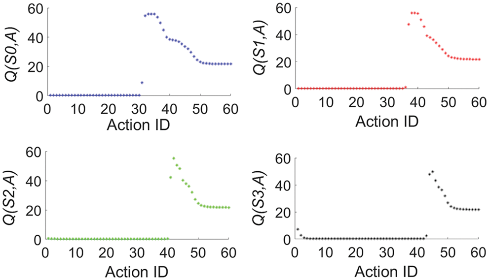
Figure 8: The predicted values Q(S,A) by neural network during the first four state transitions

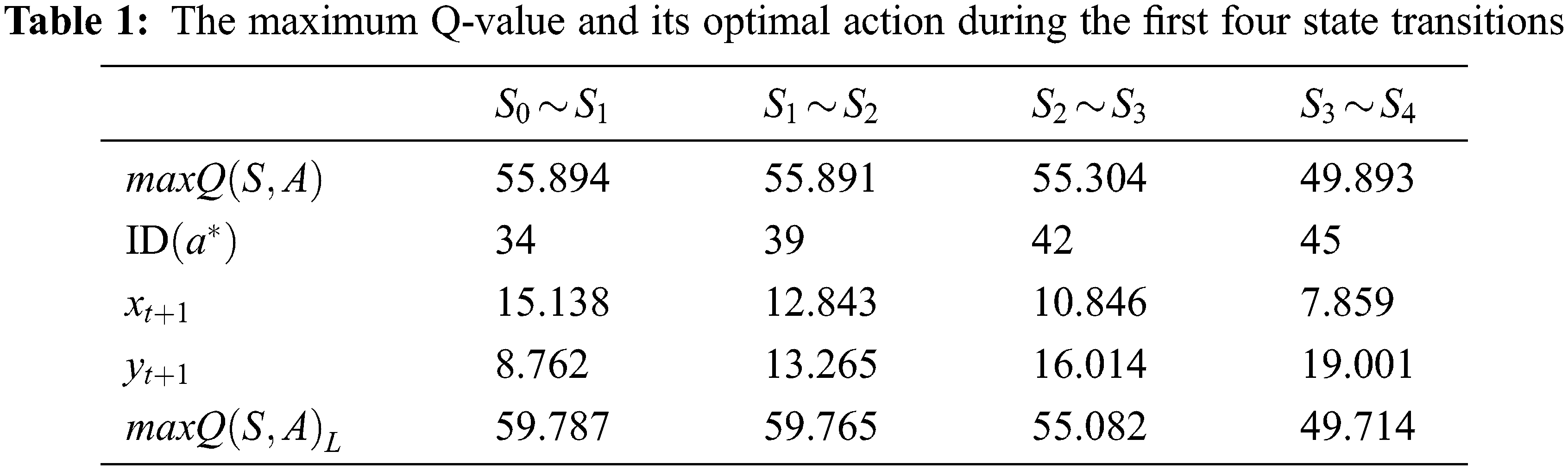
From Table 1, one can see that going from state S0 to state S4 , the predicted values Q(S,A) of the neural network are very close to the training sample label values Q(S,A)L , and the sequence numbers of optimal action corresponding to the maximums of these two values in each state are identical. This indicates that the neural network trained by Algorithm 1 has good fitting effect and has the ability to obtain the optimal policy by predicting the maximum Q-value. Since only R1 was adopted as the reward function, the optimal policy π1∗ is geared towards obtaining the most data points. For instance, from S0 state to S1 state, the neural network predicts that the maximum Q-value is 55.894, and the corresponding sequence number of optimal action is 34. This indicates that when the agent moves along the straight line with an angle of 102° (i.e. 34×3∘ )with the horizontal line from the initial point, the agent will definitely obtain the most data points in the future. The above process also demonstrates that the optimal policy obtained by the maximum Q-value is a global optimization policy. We tabulate the optimal policy π1∗ and the coordinates of all the data points obtained by this policy as Table 2.

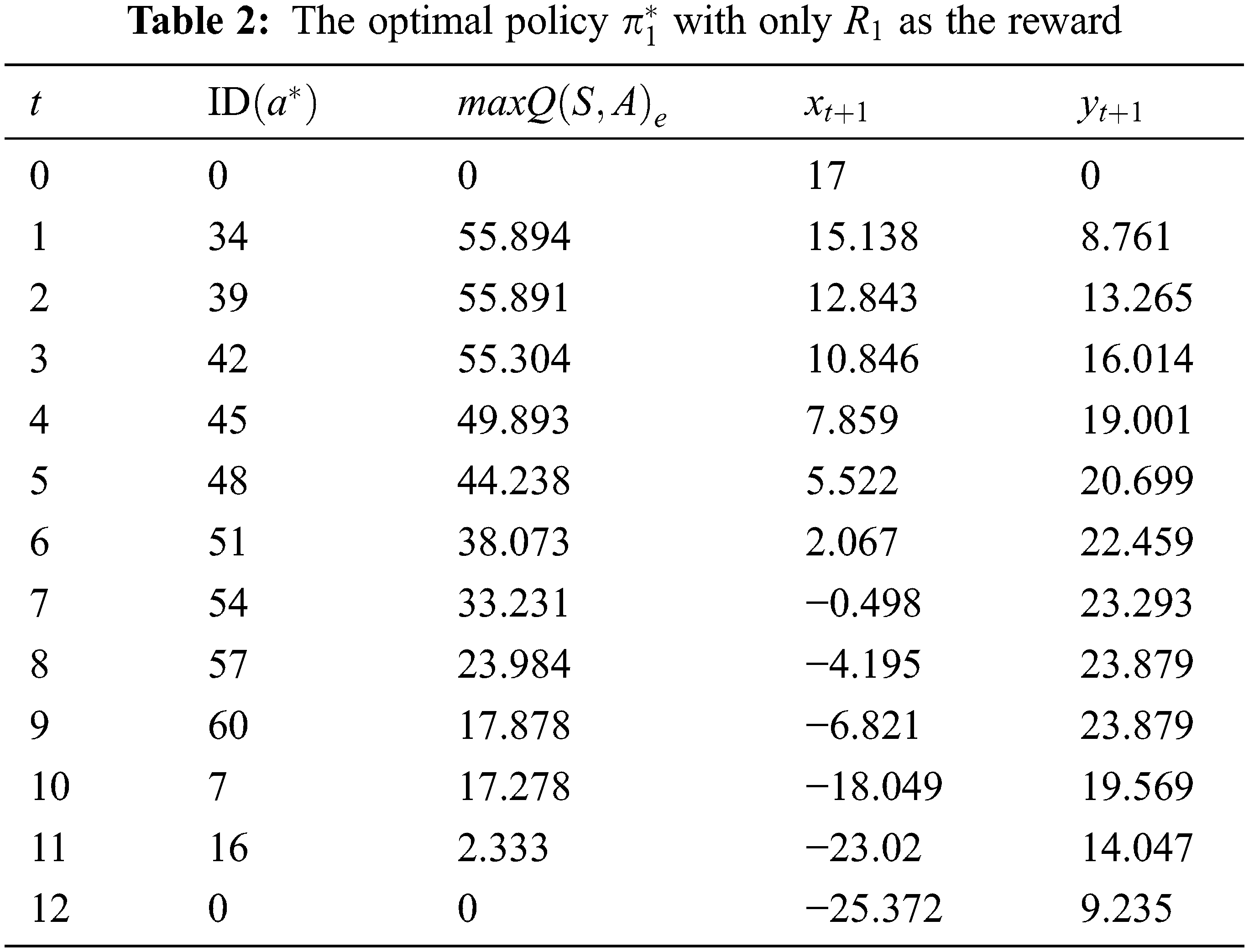
With all the data points P0⋯P12 in Table 2, one can build the knot vector , the basis functions Ni,p(u) and the control points Pcon , after which the B-spline curve expression B(u) can be obtained. We plot B(u) together with H(φ) in Fig. 9a, and then have, B(u) converted to B(φ) . In this case, B(φ) and H(φ) with respect to cam shaft angle φ are plotted in Fig. 9b.

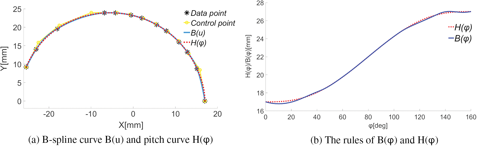
Figure 9: B-spline fitting effect of pitch curve

From Figs. 9a and 9b, one can see the followings.

When φ is within the range of 0°∼20°, due to the long distance between the first data point P1 of B-spline curve and its initial point P0 , the value of B(φ) is not only smaller than the value of H(φ) , but also exhibits a downward trend, which does not correspond with the motion law of increasing displacement of the cam follower in the rise segment. After sampling, the maximum radial error between these two curves in this range is 0.221 mm.

When φ is within the range of 20°∼110°, the B-spline curve has 9 data points and is closely distributed. The B-spline curve nearly perfectly match the pitch curve, with the maximum radial error between these two curves less than 0.002 mm.

When φ is within the range of 110°∼160°, the B-spline curve has no more than three data points, and the distribution is non-uniform. Compared with the pitch curve, the B-spline curve has a fluctuation.

Through sampling calculation, when only R1 was applied as the reward function, the average radial error between the B-spline curve obtained by the optimal policy π1∗ and the pitch curve tends to be large at 0.183 mm. This B-spline curve does not quite conform to the motion law of the cam follower and the radial profile fluctuation. As a consequence, the positions of these data points need to be further optimized.

3.2 R1+R2 Reward

To further lessen the fitting error, we take R2 together with R1 as the reward function to optimize the positions of data points. The iterative calculation in this section adopts the neural network trained in Section 3.1. In this case, steps 2 and 3 of Algorithm 1 should be removed from the iterative process. The number of data points obtained in each episode is shown in Fig. 10.

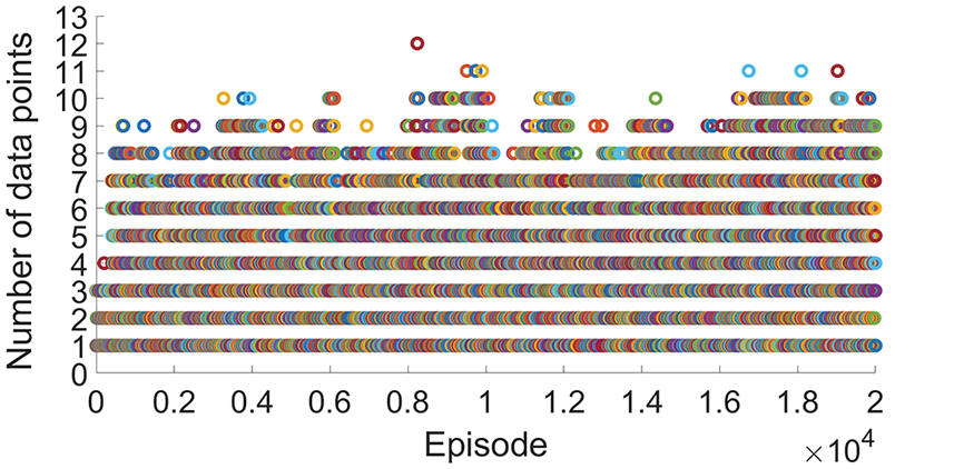
Figure 10: The number of data points obtained in each episode

As illustrated in Fig. 10, the agent can find 9 data points in the 1000-th episode. Starting from 4000th-episode, the agent can obtain 10 data points several times and find the most 12 data points in 8239th episode. After 10000 episodes, the agent can stably obtain more than 10 data points which indicates that the algorithm has converged. The convergence speed of RL learning in this section is faster than that in Section 3.1. This is because the neural network adopted in Section 3.1 only went though a basic training. At the beginning of iterative calculation, the agent clearly knows which action can obtain more data points, which contributes to the reduction of the number of blind exploration and invalid exploration. Since the reward R2 is added, Algorithm 1 now is getting additional, new training samples. After the neural network parameters are recalculated, we obtain the new optimal policy π2∗ , and present it in Table 3.

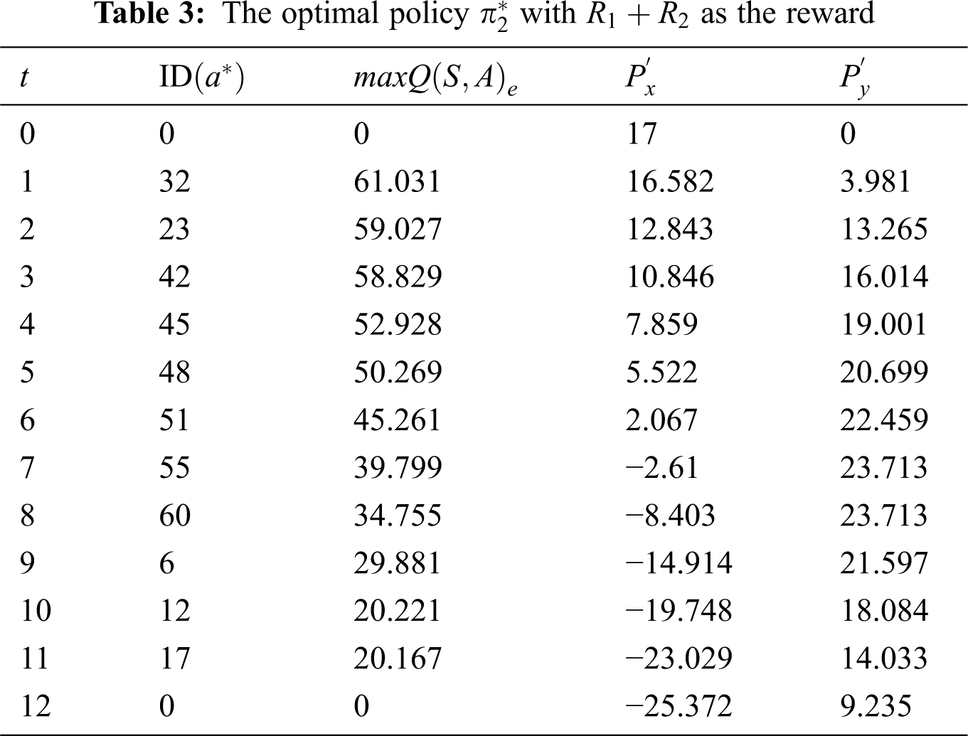
By comparing the optimal policies presented in Tables 3 and 2, one can see that the maximum number of data points obtained by π1∗ and π2∗ are the same, but the optimal actions a1∗ , a2∗ , a7∗ , a8∗ , a9∗ , a10∗ and a11∗ are different. The Q-value in Table 3 is larger than that in Table 2 due to the addition of reward function R2 . The ameliorated B-spline curve B(u) is constructed by the data points in Table 3. We plot the new B(u) together with H(φ) in Fig. 11a. Once B(u) is converted to B(φ) , we plot the rules of B(φ) and H(φ) vs. cam shaft angle φ in Fig. 11b.

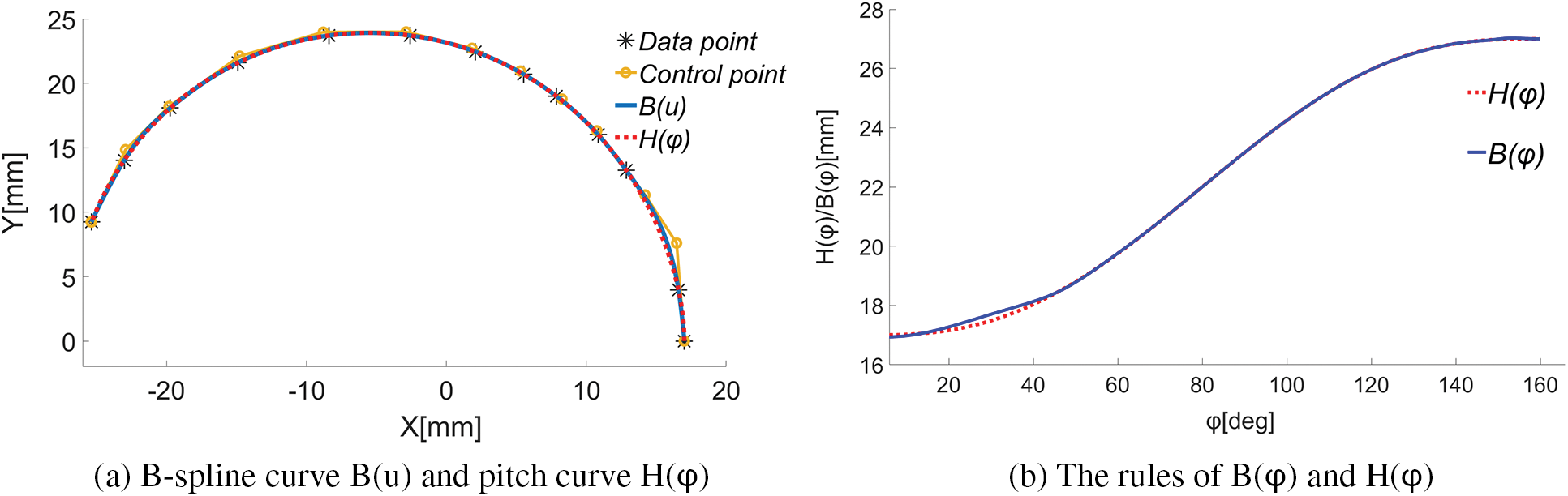
Figure 11: B-spline fitting effect of pitch curve

The data points in Fig. 11 are more evenly distributed than those in Fig. 9, and the radial error in Fig. 11 is further reduced. When φ is within the range of 0°∼20°, the B-spline curve matches the pitch curve. When φ is within the range of 20∘∖∼40∘ , although the value of B(φ) is slightly larger than H(φ) , it conforms to the motion law of increasing displacement of the cam follower in the rise segment. When φ is within the range of 40°∼140°, the B-spline curve has 8 data points, and they are uniformly distributed. The B-spline curve completely perfectly matches the pitch curve. The maximum radial error between these two curves of this range is less than 0.002 mm. When φ is within the range of 140°∼160°, the B-spline has three data points. Compared with the fitting results in Fig. 9, the profile fluctuation is substantially suppressed, with, the average radial error between the B-spline curve and the pitch curve is only 0.012 mm. This clearly indicates that after adding R2 , the Algorithm 1 can not only obtain the most data points, but also adjust the positions of these data points, with the minimal radial error between the B-spline curve constructed from these data points and the pitch curve.

As experimentally constructed in Section 4.2, the B-spline curve satisfies the motion law of the cam follower. The average radial error between the B-spline curve and the pitch curve is 0.012 mm, which is the smallest fitting error obtained under the angular division of . This value conforms with the F tolerance level of ISO2786. To further suppress the fitting error, we can use a smaller angle division value in the search of data points. Tab. 4 lists the comparison of B-spline fitting results using Algorithm 1 under three angle division values.

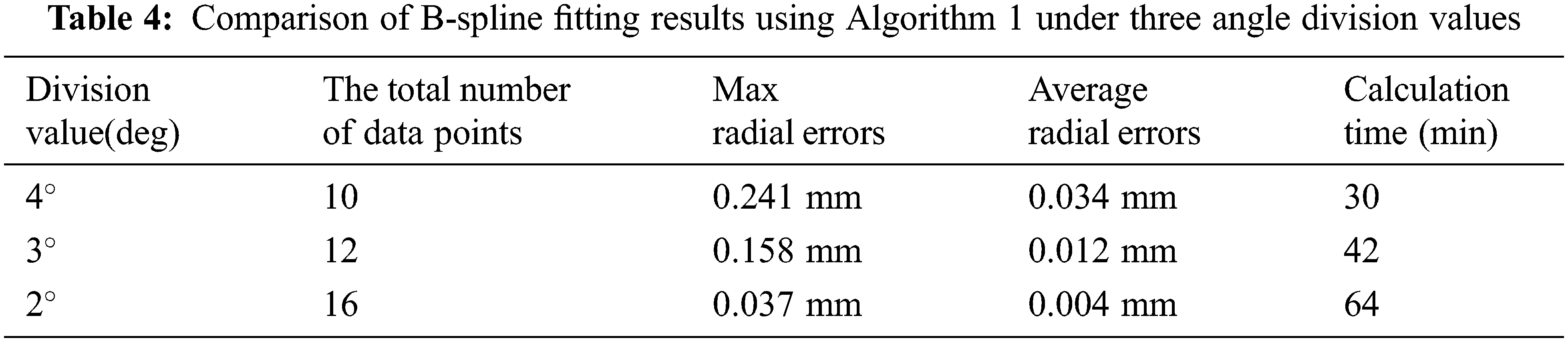
From Table 4, one can see that the smaller the angle division value is, the more data points obtained by the optimal policy. As a result, the fitting error of the B-spline curve gets even smaller a cost of longer computation time.

4  Conclusion

This paper presented an improved DDQN algorithm for fitting cam pitch curve with B-spline curve. In order to run and train the algorithm better, the environment modeling, actions set, states set, reward method and neural network were discussed in detail. This algorithm was found to automatically obtain the optimal numbers and positions of the data points on the pitch curve, and the fitting error of the B-spline curve constructed from these data points conform with the tolerance requirement. Specific contributions and discoveries were summarized below:

1. The theoretical basis of RL method for the B-spline fitting was established, and it was proved to be feasible to use RL algorithm to search for the optimal data points for curve fitting;

2. With reference to the path planning method in USV, the discrete actions set was designed to search for the optimal data points on the ideal path (the pitch curve in our case). The maximum number of data points can be controlled by scaling the angle division value of the actions set;

3. The DDQN algorithm with data point traceability was designed to accurately calculate the fitting error of the B-spline curve. The initial neural network of the proposed DDQN algorithm could be trained by a small batch of samples of which input values are randomized and output value is much smaller than the reward, to accelerate the convergence speed.

4. Two kinds of reward functions were designed in this paper. When the algorithm adopted the single objective reward function of obtaining data points, the optimal policy maximized nothing but the number of data points. When the algorithm adopted the double objective reward function of obtaining data points and calculating radial error, the optimal policy can maximize the number of data points and at the same time automatically adjust the position of data points to minimize the radial error.

Funding Statement: This research work is supported by Fujian Province Nature Science Foundation under Grant No. 2018J01553.

Conflicts of Interest: The authors declare that they have no conflicts of interest to report regarding the present study.

References

 1.  P. H. Hoang and L. Q. Ngoc, “Development of the design and fabrication system for planar cam mechanisms,” Applied Mechanics and Materials, vol. 902, no. 5, pp. 114–125, 2020. [Google Scholar]

 2.  R. L. Norton, Cam design, in Design of machinery, 5th edition. vol. 8. Los Angeles, CA, USA: McGraw-Hill Education Press, pp. 401–431, 2014. [Google Scholar]

 3.  K. Min, C. H. Lee, C. Y. Yan, W. Fan and P. C. Hu, “Six-dimensional B-spline fitting method for five-axis tool paths,” The International Journal of Advanced Manufacturing Technology, vol. 107, no. 5, pp. 2041–2054, 2020. [Google Scholar]

 4.  K. Min, Y. Y. Sun, C. H. Lee, P. C. Hu and S. S. He, “An improved B-spline fitting method with arc-length parameterization, G2-continuous blending, and quality refinement,” International Journal of Precision Engineering and Manufacturing, vol. 20, no. 11, pp. 1939–1955, 2019. [Google Scholar]

 5.  Y. K. Jiang, J. H. Chen, H. C. Zhou, J. Z. Yang, P. C. Hu et al., “Contour error modeling and compensation of CNC machining based on deep learning and reinforcement learning,” The International Journal of Advanced Manufacturing Technology, vol. 118, no. 3, pp. 1–20, 2021. [Google Scholar]

 6.  Q. Z. Bi, J. Huang, Y. A. Lu, L. M. Zhu and H. Ding, “A general, fast and robust B-spline fitting scheme for micro-line tool path under chord error constraint,” Science China Technological Sciences, vol. 62, no. 2, pp. 321–332, 2019. [Google Scholar]

 7.  S. S. He, D. J. Ou, C. Y. Yan and C. H. Lee, “A chord error conforming tool path B-spline fitting method for NC machining based on energy minimization and LSPIA,” Journal of Computational Design and Engineering, vol. 2, no. 4, pp. 218–232, 2015. [Google Scholar]

 8.  F. Yoshimoto, T. Harada and Y. Yoshimoto, “Data fitting with a spline using a real-coded genetic algorithm,” Computer-Aided Design, vol. 35, no. 8, pp. 751–760, 2003. [Google Scholar]

 9.  H. M. Kang, F. L. Chen, Y. S. Li, J. S. Deng and Z. W. Yang, “Knot calculation for spline fitting via sparse optimization,” Computer-Aided Design, vol. 58, no. 1, pp. 179–188, 2015. [Google Scholar]

10. Z. G. Yong, H. M. Kang, Z. W. Yang and Y. Gu, “The unimodality of initial B-spline approximations in spline fitting,” Communications in Mathematics and Statistics, vol. 10, no. 2, pp. 331–352, 2022. [Google Scholar]

11. S. D. Mohanty and E. Fahnestock, “Adaptive spline fitting with particle swarm optimization,” Computational Statistics, vol. 36, no. 1, pp. 155–191, 2021. [Google Scholar]

12. L. Z. Lu and S. Q. Zhao, “High-quality point sampling for B-spline fitting of parametric curves with feature recognition,” Journal of Computational and Applied Mathematics, vol. 345, no. 1, pp. 286–294, 2019. [Google Scholar]

13. Y. J. Zhao, X. Qi, Y. Ma, Z. X. Li, R. Malekian et al., “Path following optimization for an underactuated USV using smoothly-convergent deep reinforcement learning,” IEEE Transactions on Intelligent Transportation Systems, vol. 99, no. 3, pp. 1–13, 2020. [Google Scholar]

14. Y. Z. Wei, K. F. Gu, X. J. Cui, C. Z. Hao, H. G. Wang et al., “Strategies for feet massage robot to position the pelma acupoints with model predictive and real-time optimization,” International Journal of Control, vol. 14, no. 2, pp. 628–636, 2016. [Google Scholar]

15. P. Dong, Z. M. Chen, X. W. Liao and W. Yu, “A deep reinforcement learning (DRL) based approach for well-testing interpretation to evaluate reservoir parameters,” Petroleum Science, vol. 19, no. 1, pp. 264–278, 2022. [Google Scholar]

16. C. D. Boor, The representation of PP functions by B-Splines, in A practical guide of splines, 1st ed., vol. 9. New York, NY, USA: Springer-Verlag New York Inc Press, pp. 87–106, 2001. [Google Scholar]

17. N. J. Zakaria, M. I. Shapiai and N. Wahid, “A study of multiple reward function performances for vehicle collision avoidance systems applying the DQN algorithm in reinforcement learning,” Materials Science and Engineering, vol. 1176, no. 1, pp. 1–13, 2021. [Google Scholar]

18. L. Zhang, Y. M. Xie, J. Ye, T. L. Xue, J. Z. Cheng et al., “Intelligent frequency control strategy based on reinforcement learning of multi-objective collaborative reward function,” Frontiers in Energy Research, vol. 9, no. 2, pp. 1–8, 2021. [Google Scholar]

19. M. Adil, R. Ullah, S. Noor and N. Gohar, “Effect of number of neurons and layers in an artificial neural network for generalized concrete mix design,” Neural Computing and Applications, vol. 34, no. 11, pp. 1–9, 2020. [Google Scholar]

20. W. Hu, G. S. Zhang and Y. Q. Zheng, “A novel optimal control design for unknown nonlinear systems based on adaptive dynamic programming and nonlinear model predictive control,” Asian Journal of Control, vol. 24, no. 4, pp. 1638–1649, 2022. [Google Scholar]

21. K. D. Humbird, J. L. Peterson and R. G. Mcclarren, “Deep neural network initialization with decision trees,” IEEE Transactions on Neural Networks and Learning Systems, vol. 30, no. 5, pp. 1286–1295, 2018. [Google Scholar]