Depth Map Prediction of Occluded Objects Using Structure Tensor with Gain Regularization

1  Introduction

In computer vision, a depth map plays a vital role in predicting, detecting, or identifying objects. Depth map prediction is crucial for applications such as facial recognition, pose estimation, thermal detection systems, plant disease detection, and object reconstruction. The accurate depth map estimation required for effective 3D object recognition is mandatory for applications like autonomous vehicle driving and robot navigation. The disparity map of a stereo vision system represents the differences between different stereo images. Each point on a disparity map shows how all the objects in a scene move because of depth. Stereo images provide accurate, robust point correspondence images essential for discovering local appearance traits. For successful depth determination, a single image must include atmospheric influences, line angles, and position. Stereo estimates dense depth maps local disparity alone.

1.1 Stereo Vision

Stereo vision aids in generating depth maps for the input images taken using a stereo vision-based camera. The following Fig. 1 represents the stereo vision principle [1]. The depth map depicts the triangular similarity exhibited by the rays from multiple viewpoints, similar to human visual perception.

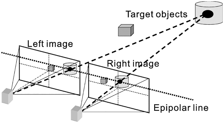
Figure 1: Stereo vision principle

In stereo vision images, the depth maps contain information related to pixel correspondence. The point pixel coordinates of both left and right images aid a better reconstruction process. Matching the pixel coordinates with left and right images will improve depth map generation. The depth map generation considers the distance of the pixels in the given scene by computing the disparity between the left and right images. The intersection of rays gives the 3D location of objects with their gradient measures.

1.2 Monocular and Binocular Depth Map Estimation

The monocular depth cue estimation involves various parameters like lightning conditions, height, the texture of the object, linear or aerial perspective (convergence of parallel edges), oculomotor (accommodation), and interposition. The binocular depth cues estimation involves the parameters such as convergence and binocular disparity. The monocular view obtained by the single eye has a reduced field of vision and depth perception. In contrast, the binocular views obtained by both eyes with the stereoscopic method produce the depth map for 3D reconstruction for both eyes.

1.3 3D Reconstruction with Intensity Variation

The depth map computation of gray-coded 2D images exploits varying pixel intensities. The darker regions in the depth map represent objects farther from the camera position. In contrast, the less dark or lighter regions are bound to be nearer to the camera position. The variance in the object’s distance in the scene aids in differentiating the objects based on the distance from the camera position.

1.4 3D Reconstruction with Occlusion Detection

The presence of occluded objects may deteriorate the overall performance of 3D reconstruction. The traditional 3D reconstruction pipeline involves the given input image, the correspondence depth obtained through the multi-view images, and the depth map estimation with the depth fusion method.

1.5 Depth Map Highlighting Occlusion Region for 3D Reconstruction

This work focuses on the depth estimation of a stereo vision image. A novel modified stereo block matching algorithm enabled the practical computation of disparity maps, where this disparity estimation process considers only the occluded image regions or lack texture portions. The process of 3D reconstruction requires dense depth maps beforehand. So, a proposed dense disparity map estimation method could detect occlusion effectively. The occluded objects are determined by the proposed plane fitting and gradient-based block-matching algorithm.

The Contributions of this work are as follows

1.    The correspondence point pixel computation accurately uses an improved stereo-matching method.

2.    An improved stereo matching and gradient-based Structure Tensor method compute the minimum matching cost.

3.    Generation and refinement of disparity map using smoothness function.

4.    The improved depth map with gradient measure shows the apparent differentiation effect among the objects.

The rest of the paper describes as follows, Section 2 deals with the various existing approaches for stereo image reconstruction in the presence of occlusion. Moreover, Section 3 explains the proposed depth map prediction architecture. Section 4 proposes an improved algorithm for the depth map prediction problem. Section 5 gives the experimental setup, Section 6 discusses the results obtained through the simulation, and Section 7 concludes the work.

2  Related Work

This section narrates various existing approaches toward the 3D reconstruction process in stereo images, with depth map estimation. Rogge et al. [2] have considered light-field (LF) images and proposed a depth estimation technique with multi-stereo matching and machine-learning techniques. Their initial depth estimation was estimated using a block-based stereo-matching algorithm. Engagement of smaller input batch sizes, the inference time is reduced. Aslam et al. [3] have proposed a method for generating depth maps based on the pixel-to-pixel matching algorithm for the two images in stereo vision. While calculating the depth estimation, they found the corresponding pixels in different views by identifying the point of correspondence for the same 3D points. Then the depth information was calculated by matching pixels for the best pixel, resolving the conflicts between the current and previous pixel values. The precise identification of the different object's gradient levels deteriorates the overall performance due to the presence of occluded objects.

Li et al. [4] proposed a model to estimate depth for RGB images with different learning methods of supervised, unsupervised and sparse sample guidance methods. They have addressed the problem of dynamic objects and occluded areas by learning a mask or through segmentation with a CNN-based architecture. However, they have yet to consider the fusion of segmentation with the geometric or color constraints between stereo pairs or adjacent frames. Dong et al. [5] have proposed a method for automatically generating depth maps from 2D to 3D using the global gradient depth method. They produced a closer depth of the area that contains more details, often drawing the viewer's attention. However, they still need to produce the improved rendering of objects due to the teething difficulties in improvising the quality of the depth map with an appropriate filter.

Liu et al. [6] proposed an end-to-end network and Domain Invariant Feature Descriptor-Net (DIFD-Net) with features that dynamically change concerning the moving images. They have considered the cross-domain sources where the images from Structure from Motion (SFM) and images of aerial photography images divided into patches. The RANdomSAmple Consensus (RANSAC) algorithm analyzes the difference between the camera and extracted images for the irregular observed patches. However, they have claimed that severe occlusion and distortion were beyond the human’s visual perception level. Liu et al. [7] have focused on learning the feature descriptors of 2D image patches and 3D point cloud volumes using a Perspective-n-Point algorithm(PnP) to find the 2D–3D correspondence. They have applied a key point detector for point correspondence. The 2D and 3D (Generative Adversarial Network)3D-GAN-Net were employed to extract the multi-domain feature descriptors. Eigen et al. [8] proposed a methodology for predicting coarse global information and local refinement of depth maps for understanding the 3D geometry of the scene. The fine-scale network has learned the details of object boundaries and wall edges for the points with no depth values. The multi-scale deep network learned from large training datasets aids in the handling of pixels with no depth values. Their method could have concentrated on the surface boundaries with sharp transitions.

Durner et al. [9] have proposed an Instant Stereo Transformer (INSTR) algorithm to find the object boundaries and extract them without prior knowledge of semantic or geometric information about objects. Surmise object boundaries for better realism of dense depth maps. The segmentation of various textures/shaped objects was also grasped accurately, even for unseen objects. The stereo-aided robotic vision also commissions depth map computation. Some of the widely used disparity optimization algorithms are belief propagation [10,11] Graph Cuts, and Dynamic Programming [12]. The Sum of Squared Difference (SSD) or Sum of Absolute Difference (SAD) is the primary similarity metric. The SSD/SAD represent large blobs of disparities that lack texture. The window must be more significant to distinguish the individual characteristics of an image. On the other hand, if the window is too large, many patches may share similar characteristics and result in unwanted mismatches.The strength and weaknesses of various approaches for stereo image reconstruction with occlusion were analyzed.

There are also several solutions for stereo-image depth estimation. Eigen et al. [8] perform depth prediction for finding the object boundary using the multi-scale deep network. A semi-global block-matching algorithm can detect the object shape boundaries. A structure tensor method determines the sharp transitions. The Middlebury stereo dataset uses structure lighting techniques to capture depth for the occluded and non-occluded objects. Our method uses such datasets to provide dense depth maps concentrating object boundaries with sharp transitions even in occlusion. A plane-fitting filter would recognize whether all pixels lie on the same plane.

3  Proposed Depth Map Prediction Architecture

3.1 Logical Steps

The proposed approach has considered the input stereo images taken from the left and suitable cameras under various lighting conditions and angles. The generation of the depth map for the objects requires different camera calibration parameters. The depth map calculation aids the disparity computation of the scene to have an apparent effect on the quality of 3D reconstruction. The practical computation of the disparity map aids in detecting/identifying the occluded pixel's information.

The proposed occlusion detection describes the Input and Output of the model below:

Input:Img={ImgL,ImgR} left and the right image obtained from the stereo camera

Output: Object depth map

For each pixel P(x,y), its disparity (D) will fall in {dmin,dmax}. Moreover, Os∈{T,F} it will represent the presence of occlusion.

Considered Dataset: Middlebury Stereo dataset [13,14].

The proposed approach has been divided into various logical steps, as given below:

Step 1: Disparity Estimation

a)   Calculating the disparity based on the displacement in the pixels with the Modified Semi Global Block Matching Algorithm (MSGBM) by variable window/ block size and several disparities.

b)   It identifies the foreground/background objects with high and low disparity values.

c)   The consistency check between the left and right images would reveal the number of occluded pixels.

Step 2: Gradient Estimation with Structure Tensor method

a)   will find the gradients of the objects

b)   A novel Plane Fitting Filter has been applied to identify the gradients/planar of every object for object shape identification.

Step 3: Estimating the Disparity Map from the resultant values of steps 1 and 2.

3.2 Proposed Depth Map Prediction Architecture

This section describes the proposed architecture for disparity estimation of stereo images by block matching algorithm with gradient-based structure tensor method.

The computation of the method's reliability determines the object planar using the plane fitting filter method. The occlusion pixel detection involves the consistency check in one direction to compute the disparity map. As a result, to have minimum computing cost in similarity metrics computation. The below figure shows the proposed architecture (Fig. 2).

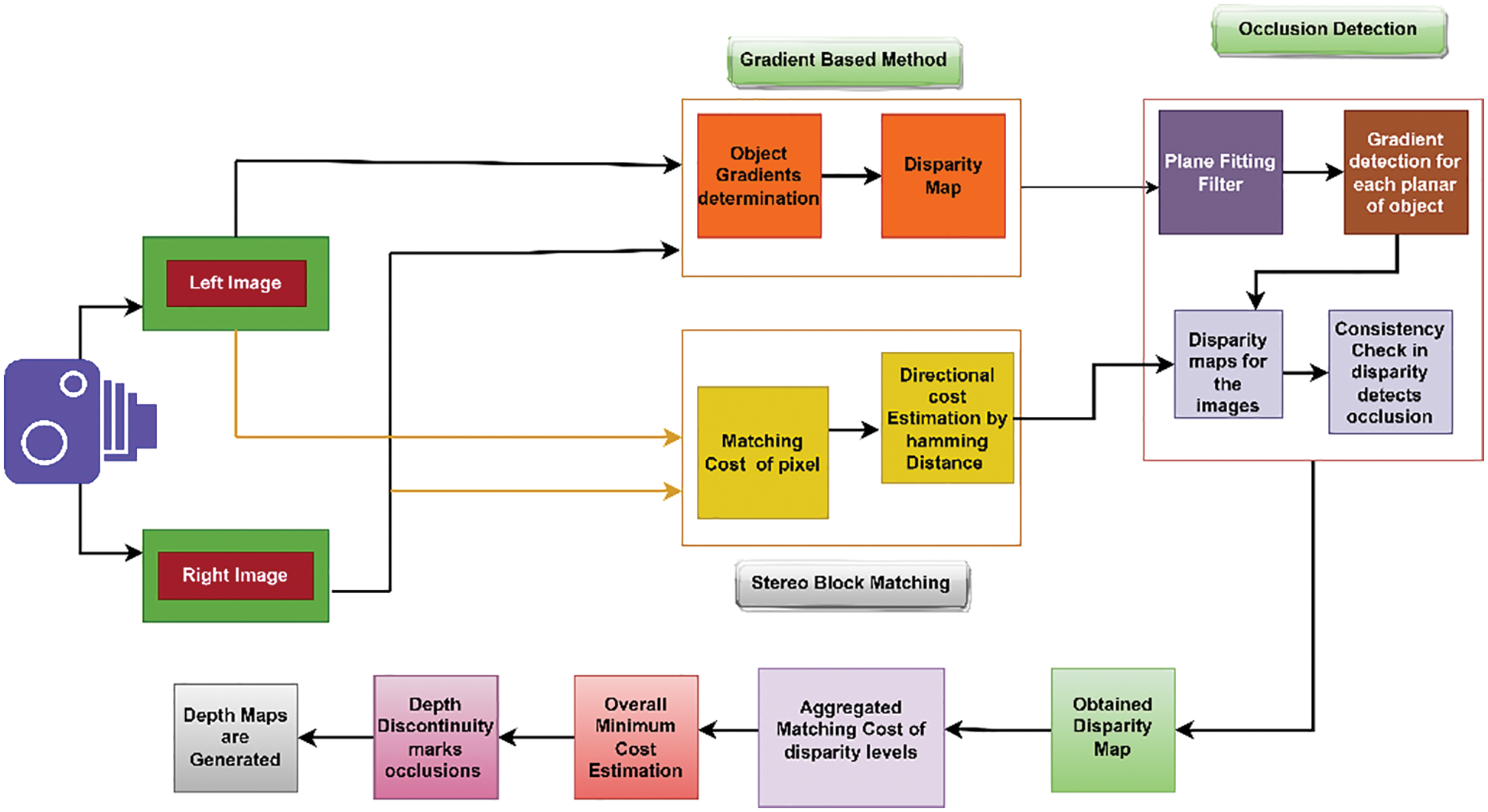
Figure 2: Architecture diagram for the proposed algorithm

4  Proposed Depth Map Prediction Algorithm

The proposed depth map computation involves the following two modules.

1.    Disparity estimation with modified block matching algorithm

2.    Edge identification with a modified gradient-based algorithm

4.1 Modified Disparity Estimation Algorithm

The occurrence of occlusion in the input image might affect the transformation process of 2D to 3D object reconstruction with a reduced plausibility effect in the rendering process.

Our modified block-matching approach undertakes the following steps for computing the disparity map:

1.    Cost computation of matching points with the semi-global algorithm

2.    Aggregation of pixels with disparity values

3.    Finding the minimal aggregated disparity cost

Most conventional window-based algorithms would compute the disparity map based on aggregating pixels with disparity values. The implicit smoothness assumption for disparity computation was computed based on intensity values in finite frames/windows/blocks. The following sections narrate the three significant steps followed in our proposed block-matching algorithm.

4.1.1 Cost Computation of Matching Points with a Semi-Global Algorithm

We use various stereo block matching algorithms with varying window sizes to compute disparity maps. We have exploited various transformation techniques to detect the disparity between the stereo images for improved block matching. We have chosen the Centre Symmetric Census Transform (CSCT) [15] to identify pixel mismatches with varying window sizes. The center census transform method in Fig. 3 [16] has resulted in pixel variations between the center of the window and its neighborhood pixels. We have exploited various cost metrics to quantify the pixel-based mismatch, which includes Squared Intensity differences (SID), Absolute Intensity Difference (AID), Mean Squared Error (MSE), and Binary matching costs [17]. Sometimes, the cost metrics might be insensitive to variations in camera gain or bias. The gradient-based measures, such as the structure tensor method, could determine the intensity orientation around specific neighborhood points. The neighboring points calculated the pixel-dominant orientation and the shape measures of the objects.

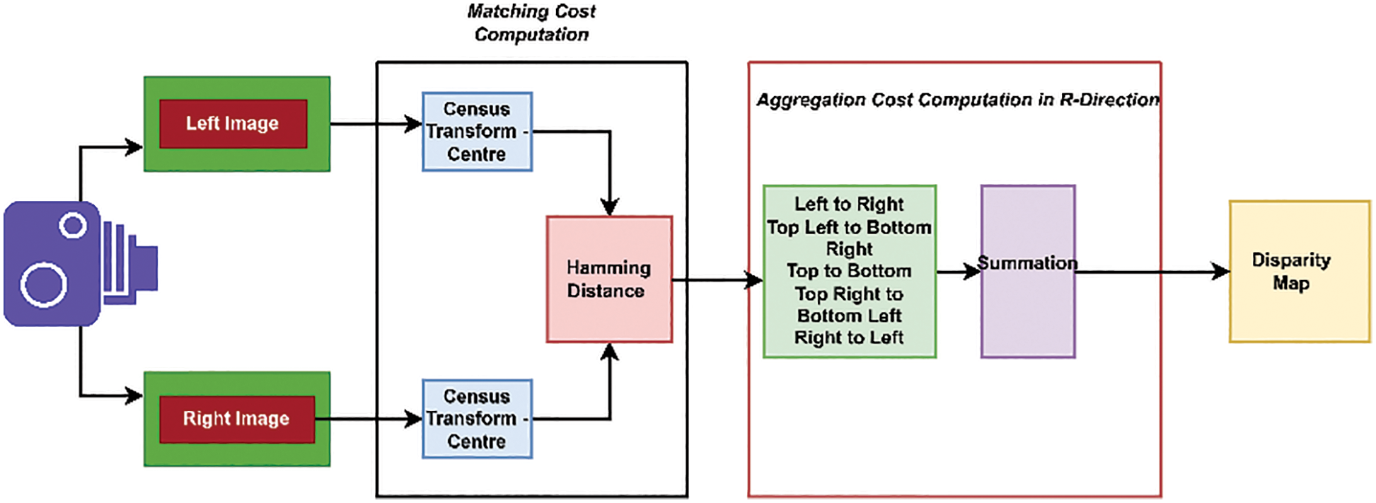
Figure 3: Modified semi global block matching algorithm (SGBM) for disparity estimation

Computation of detected pixel based on the consistency check done in one direction, i.e., left-to-right direction, to minimize the overall computation cost in generating the disparity map. The proposed block matching algorithm has enabled matching the macroblocks in the left and right images to find the corresponding match. The pixel displacement was estimated using variable-sized windows with the block-matching method. The input stereo images Img={ImgLImgR} were captured with a stereo camera with variable focal length, baseline distance, and depth of field. The modified stereo block matching algorithm computed the correspondence match in the input images with varying window sizes, such as 3, 5, and 7. For every pixel P(x,y), the Block Matching Cost (BMC) (as shown in Eq.(1)) uses the statistical similarity metric for each corresponding window of Window1 and Window2 in the image pair using SSD(Sum of Squared Differences).

BMCSSD=∑x,y|Window1(x,y)−Window2(x,y)|2(1)

With the block size (B), Currij(current right image), and Refij (left reference image), the correspondence match was found using the similarity metric of Mean Squared Error (MSE) (as shown in Eq. (2)).

MSE=1B2∑i=0n−1∑j=0n−1(Currij−Refij)2(2)

Then the mismatched pixels from the set of block images were calculated using the difference operator among the image pixels. The block matching algorithm aims to find the disparity D(x,y) measure for each pixel x and y to represent the contours of the objects in the scene. We have converted the stereo images into rectified images with the Epipolar line matching technique [18]. The pixel-wise matching was done for the stereo-rectified images to compute the disparity map. The horizontal 1D alignment of pixels in the stereo-rectified images will be amenable for the computation of correspondence pixel mismatch with interference. The pixels of the stereo image pair with pixel coordinates P(x,y) for ImgL,and ImgR performs disparity calculation (D). The Cost function to calculate the disparity (as shown in Eq.(3)).

Cost(D)=∑PDis(P,Dp)+∑P,Q∈NReg(P,Dp,Q,Dq)(3)

The cost function for the disparity  costs(D) was estimated for the pixels P and Q with a disparity Dp and Dq, respectively, for the neighborhood Pixels N. The pixel-wise dissimilarity cost Dis(P,Dp) was calculated among the pixels. Reg(P,Dp,Q,Dq) represents the regularization cost that penalizes the difference or jumps in a disparity between adjacent pixels. Hamming distance measures D disparity levels for (P to D + P) pixel positions in the right picture, assuming that the matching cost for a specific pixel position p in the left image is known. The matching cost, represented by the notation Cost (P, D), is computed for each disparity level at each pixel position, P. Hence the improved block matching considers various factors for occlusion detection. The pixel detection is carried in one-way, i.e., left to the right direction, to identify the occluded pixels in the disparity map with minimum cost.

4.1.2 Aggregation of Pixels with Disparity Values

The Mean Relative Error (MRE), Mean Squared Error (MSE), and Root Mean Squared Error (RMSE) are some of the existing similarity measures used in best-depth estimation for measuring details such as pixel intensity, disparity, edges, and texture. The winning similarity measure has a higher discriminative for wrong or corrupted disparity value and a narrow minimum around the correct disparity value. The aggregated matching cost has considered neighborhood pixels (as shown in Eq.(4)).

Agg(P,D)=∑rImgLr(P,D)(4)

Aggregated matching cost Agg(P,D) from each pixel position P in r directions calculated for the coordinates (x,y) and disparity D for the left image ImgLr(P,D). The Aggregated matching cost computation through window-based stereo used either the gaussian kernel or convolution with box. The directions for predicting pixel corruption levels ranging from noise to the occlusions were determined using five different direction traversal, i.e., right to left, left to right, top left to the right corner, top to bottom, and top right to left corner. The computation of aggregated cost along r directions (ImgLr) has exploited the discontinuities in depth with a change in the intensity gradient.

ImgLr(P,D)=cost(P,D)+min(ImgLr(P−r,D),ImgLr(P−r,D−1)+PR1,

ImgLr(P−r,D+1)+PR1,miniImgLr(P−r,i)+PR2)−minKImgLr(P−r,k)(5)

where, ImgLr(P,D) = pixel x current cost and disparity D in the direction r

cost(P,D) = pixel x matching cost and disparity D

ImgLr(P−r,D+1) = previous cost of the pixel at disparity D + 1in the direction r

ImgLr(P−r,D−1) = previous cost of the pixel at disparity D − 1in the direction r

miniImgLr(P−r,i) = minimum cost of the pixel in the r direction for the previous computation

PR1and PR2 is the penalty parameters in regularization terms, responsible for finding intensity discontinuity I described as

Reg(Dp,Dq)={result 0 when Dp=DqresultDp when |Dp−Dq|equal to 1resultDq when |Dp−Dq|when greater than 1(6)

Then the below formula shows the computation of each pixel disparity cost

D∗(P)=argminD Agg(P,D)(7)

4.1.3 Finding the Minimal Aggregated Disparity Cost

At most, the pixel in one image should correspond to one pixel in another image. In our proposed disparity estimation approach, the aggregated disparity cost considers a lower value of threshold five due to the occurrence of occlusion in computing the depth map.The estimation of global disparity cost utilizes both graph cut [19] and the uniqueness constraint. The following flowchart (Fig. 4) depicts the modified approach for estimating disparity.

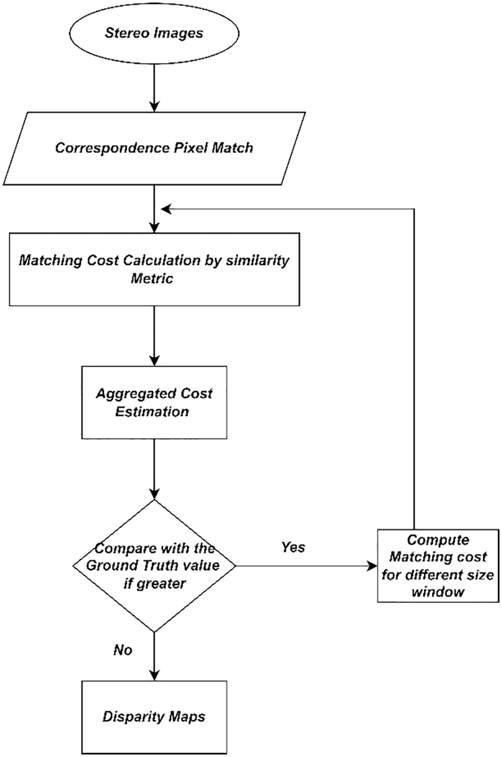
Figure 4: Flowchart of the modified disparity estimation algorithm

Modified Disparity Estimation Algorithm

Input: Stereo Images Img={ImgL,ImgR}

Output: To Estimate Disparity Map

Repeat Block matching with varying windows

       Find Correspondence pixel Match with a displacement pixel value

       Matching Cost Estimation (SSD)

       Pixel Mismatch due to occlusion/noise, then Compare with the ground truth value

Until: Determine Minimal Matching Cost among all Disparity values

Require: Consistency check in one direction of disparity map to avoid the cost computation time overhead

Ensure: Calculate Cost Volumes CostL(Pi,S) and CostR(Pi′,S)

pixel Pi and Pi′ denotes corresponding points with coordinates of the left and right image planes Pi=[xqL,yqL]T and the right coordinate Pi′=[xqR,yqR]T

disparity coordinates of cost volumes, SL of the left and SR of right disparity

Perform the cost-filtering algorithm using SAD to find minimal cost Cost−L(q,s) and Cost−R(q,s)

Occluded pixel detection

OccqL={occlusionifSL[xqL,yqL]≠SR(xqL−SqL,yqL)nonocclusionelsewhere

Return: OccqL is the output occlusion map.

If, OccqL=occlusion, return:the estimated SqLvalue is uncertain

Else

Replace any gap-filling with a post-processing procedure

Returns: Disparity Map with disparity D in the range of {dmin,dmax}

4.2 Edge Identification with a Modified Gradient-Based Algorithm

The following steps followed in the modified gradient-based algorithm:

1.    Gradient-Based Structure Tensor

2.    Plane fitting filter

3.    Occlusion Detection and Cost Computation

As different filters have different effects on the gradient estimation, the proposed edge identification method made to choose the appropriate filter concerning the inter-object distance, window size, and neighborhood pixels for occlusion detection.

4.2.1 Gradient-Based Structure Tensor

The gradient-based method effectively determines the values for every object in the vertical plane with the horizontal gradient operator. The conventional method detects the optimal edges of the objects with canny edge detection [20] followed by the threshold operation. The proposed method uses a modified structure tensor method [21] to detect the gradient of objects along with the magnitude. The gradient measure is a baseline for predicting the object plane in object identification. Gradient information is represented as a multi-dimensional array to describe local gradient characteristics precisely. Following the gradient calculation, the direction of the gradient was determined solely by the pixel values. The matching cost is based on the window size and gradient information ∇D=Dx,Dy of D within the window W centered at point q with pixel coordinates of pi(x,y)checked for consistency in the pixel match.

Plane fitting filter

The filter takes advantage of the fact that the target disparity function Sq, is assumed to be locally embedded in a geometric plane with a gradient of Dq. This filter was inspired partly by the concept presented in [22] and is defined as follows in Eq.(8).

Dq=∑P∈Nρe−|πp−Dq|2σπ22−|∇Dp−∇Dq|2σk22πp(∇Dp,Dp,q)(8)

Where Dq is the filter output, πp=πp(∇Dp,Dp,q) which is the predictor value,

gradient ∇Dp, Dp are the disparity value at pixel q, Spis the known gradient value.

The plane fitting filter’s intrinsic parameter σπ controls the affinity between the estimated value πp and the given value Dq. The intrinsic parameter gets a value of 5, and another intrinsic parameter σk also, get a valueof 0.2. The weight exp(−|πp−Dq|22σπ2) has become zero whenever the gradients of the desired function S in the pixels q and p were noticeably distinct from each other and belonging to different planes. The dimension of the local neighborhood window Nρ is 15 × 15. In principle, post-processing techniques can include sub-pixel disparity improvement. The following flowchart (Fig. 5) depicts the modified edge identification with the gradient estimation.

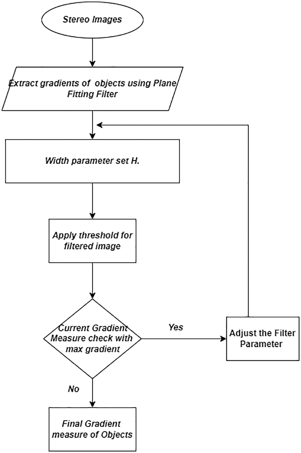
Figure 5: Flowchart of the modified gradient estimation algorithm

4.2.2 Occlusion Detection and Cost Computation

An adaptive median filtering process aids in differentiating object pixels from occlusion, identifying the corrupted and uncorrupted windows through the filtering process engaged replacement with a median value. Some of the existing stereo algorithms may treat noise as the occlusion in stereo images, but our proposed approach was bound to consider the occluded using the modified correspondence match.

Edge identification with a modified gradient-based algorithm

Input: Stereo Images Img={ImgL,ImgR}

Constraints: gradient tensor of shape (h,w,c) where c >= 1, h = height, w = width, c = constant.

Block size: block sizes for left and right are 5 or 7

Similarity Measure Function: Check the similarity measure between two tensors of the same object shape

If tensor measure = = the same object

Return Matching Cost

Else

Return Error

5  Experimental Setup

The Dell Precision T3630 Workstation with Intel i7-9700, 8 Core, 12 MB Cache, 3.0 Ghz, 4.7 GHz, Turbo w/UHD Graphics 630, Precision 3630 Tower with 850W up to 90% efficient PSU (80Plus Gold) with SD card. 16 GB DDR4 2666MHz UDIMM Non-ECC Memory, 3.5 inches 1 TB 7200rpm SATA HDD, M.2 256 GB PCIe NVMe Class 40 SSD, Nvidia RTX 2080Ti 11 GB Graphic Card used for the simulation.

The disparity map calculated through the modified block matching algorithm and gradient measure has been compared with the ground truth to identify the matching cost and occlusion percentage. In the proposed approach, the matching cost has been kept minimum by maintaining the smaller window size to handle the noisy and occluded pixels.The proposed stereo block matching algorithm allowed for comparison with the following state-of-the-art approaches for their ability to compute disparity maps.

1.    Semi Global Block Matching Algorithm (SGBM)

2.    SGBM with Graph Cut (GC) method

3.    SGBM with SLIC (Simple Linear Iterative Clustering) method

We have considered the Middlebury stereo datasets [13,14] of Tsukuba, cones, sawtooth, venus, and a teddy for developing a model of structure tensor with a plane-fitting filter for disparity computation to calculate the depth maps. Test the modified stereo block matching method with the datasets mentioned above to claim its least cost in reconstructing the dense depth maps.

Figs. 6 and 7 represent disparity maps of the proposed algorithm. Near object takes a higher disparity value than distant objects from the camera. The default value set is 64 from a range of 8 to 128. The disparity level increased to improve the depth calculation of the objects. The threshold value falls between zero and hundred for the level of uniqueness, whereas the typical range falls between 5 to 15. Lowering the value of the uniqueness threshold has resulted in finding more reliable disparities.

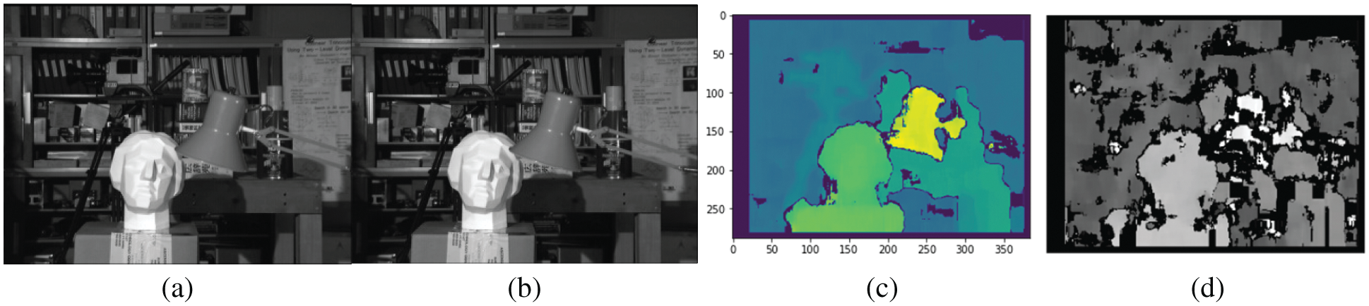
Figure 6: a) Left b) Right Image c) and d) Disparity maps obtained by block matching algorithm

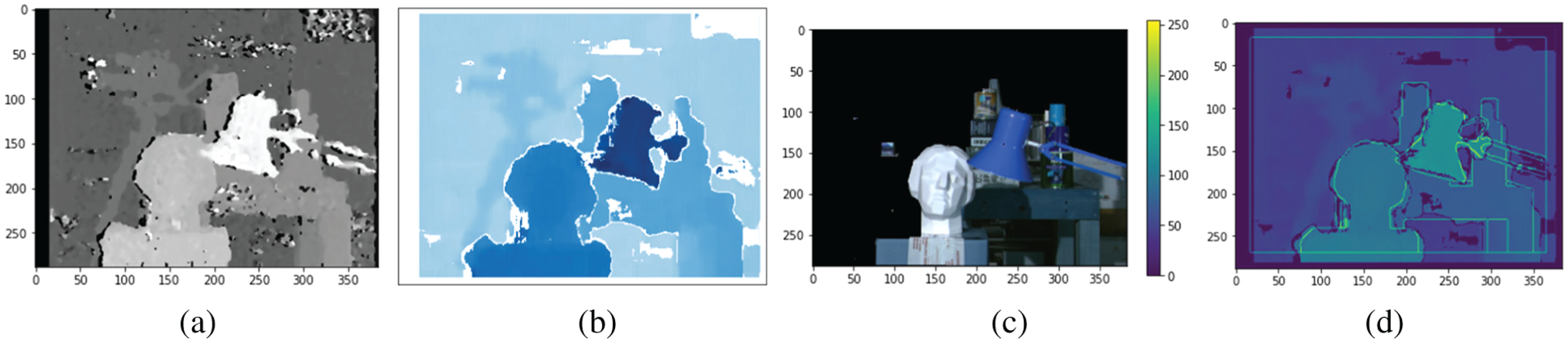
Figure 7: a) SGBM Disparity Map b) Border occlusion and unfilled region in white regions c) Occluded object visibility relative to the colorbar with disparity level d) Object gradient and disparity map combined

Figs. 8 and 9 describe the output obtained from the proposed method, which determines the gradient measure of each object present in the image. Compare the ground truth value with the proposed method to obtain the minimum matching cost value of matching metrics with a window size of 5 and block size of 15, with num disparities = 16, and the predictor value in the gradient measure as 0.001.

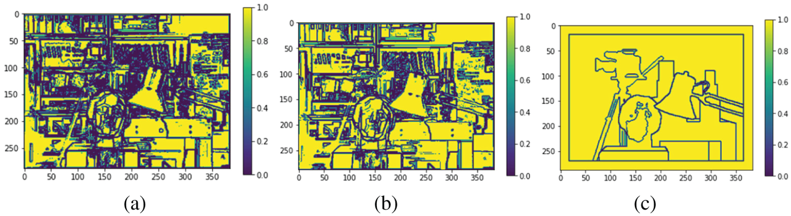
Figure 8: a) left Image b) Right Image c) Ground Truth Image obtained from gradient-based algorithm

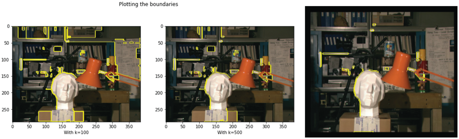
Figure 9: Occlusion detection of objects with varying levels of parameter k along with the object edges

6  Results

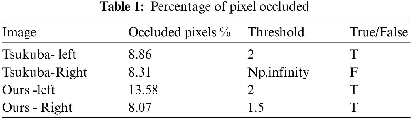
We have created our dataset with the GigE stereo vision camera setup with varied lighting conditions. The front lighting with varying exposure was captured and compared with the benchmark dataset with varying thresholds. The occluded pixels were notated as Os∈{T,F}.

We observed that the Middlebury stereo has very few images with occluded objects, which made the attainment of gain cumbersome. Considering this gain, we have created our dataset with occlusion using the structured lighting technique. The regularization term in the graph cut algorithm for handling occlusion in the optimization process has been evaluated for different smoothing coefficients in Fig. 10. Table 1 describes the percentage of the pixels occluded for the benchmark Tsukuba [13,14], and our dataset.

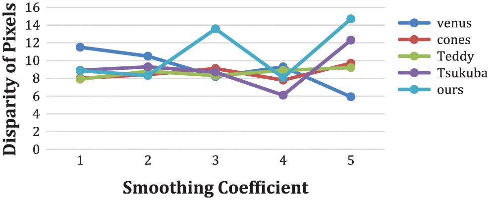
Figure 10: Smoothing performance coefficient with disparity pixels for various image pairs

The proposed method has exploited the disparity pixels to obtain better depth maps for Middlebury datasets. Fig. 11 shows the maximum gain from the occluded pixels of various image pairs and the minimum gain taken from the state-of-the-art datasets. The maximum gain in the real-world dataset captured using structured lighting with varying focal lengths and baseline values concerning the relative camera parameters determines the efficient or dense disparity maps.

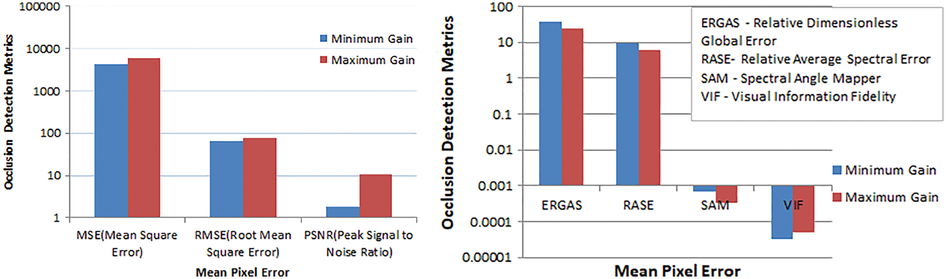
Figure 11: Gain Attainment Score for similarity metrics

Fig. 12 represents the performance score obtained by the various stereo algorithms against the Middlebury datasets about the execution time for the various image pairs.

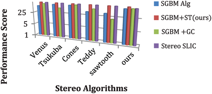
Figure 12: Performance score of various stereo algorithms

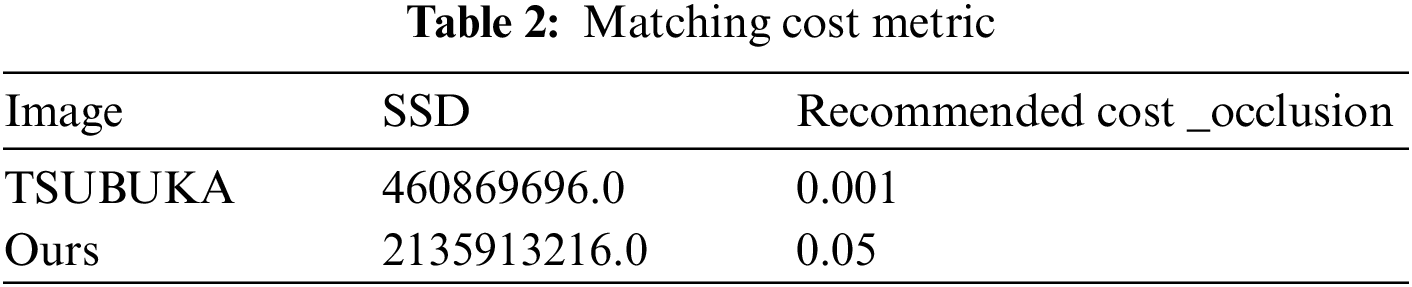
The below Table 2 shows the matching cost value from various metrics, among which the SSD score measured for one image benchmark image pair and our image pair compared and depicted in the table.

The following Table 3 represents the evaluation metrics of a performance score and bad pixel match errors given in percentage. The following figure (Fig. 13) compares various existing stereo block matching approaches regarding detection error % and performance score.

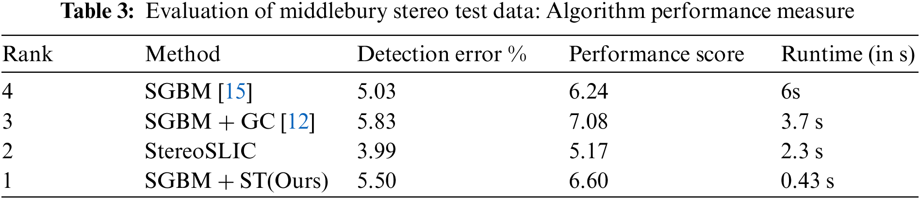
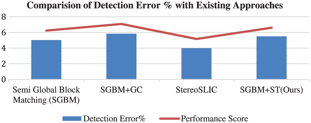
Figure 13: Detection error % and performance score of various stereo block matching algorithms

7  Conclusion and Future Work

3D reconstruction involves the computation of a depth map from the 2D scene. The presence of occlusion marks the resultant depth maps as inaccurate. This work focused on developing an algorithm to calculate depth maps useful for robotic navigation. Obtained the disparity map through the modified stereo block matching algorithm preprocessed with the structure tensor method for gradient information and plane fitting filter for the effective discrimination of object planes. Evaluate the proposed structure tensor-based block matching approach and the established state-of-the-art block matching for comparison.

The results demonstrated that the proposed approach outperforms the existing approaches in terms of reduced processing time and more accurate detection of occlusions. In our proposed approach, the sparser disparities result in ineffective handling of the reconstruction process. In future work, we propose filling occlusion areas with a novel approach that improves the apparent effect of object shapes differentiation and fusing depth maps into a volumetric and point-cloud data representation structure. A dense reconstruction of the scene and improvement in the geometry of the reconstructed 3D model.

Funding Statement: The authors received no specific funding for this study.

Conflicts of Interest: The authors declare that they have no conflicts of interest to report regarding the present study.

References

1. M. Hariyama, N. Yokoyama and M. Kameyama, “Design of a trinocular-stereo-vision VLSI processor based on optimal scheduling,” IEICE Transactions on Electronics, vol. 91, no. 4, pp. 479–486, 2008. [Google Scholar]

2. S. Rogge, I. Schiopu and A. Munteanu, “Depth estimation for light-field images using stereo matching and convolutional neural networks,” Sensors, vol. 20, no. 21, pp. 6188, 2020. [Google Scholar] [PubMed]

3. A. Aslam and M. Ansari, “Depth-map generation using pixel matching in stereoscopic pair of images,” arXiv preprint arXiv:1902.03471, 2019. [Google Scholar]

4. Q. Li, J. Zhu, J. Liu, R. Cao, Q. Li et al., “Deep learning based monocular depth prediction: Datasets, methods, and applications,” arXiv:2011.04123v1 [cs.CV], 2020. [Google Scholar]

5. H. Dong, S. Yin, W. Xu, Z. Zhang, R. Shi et al., “An automatic depth map generation for 2D-to-3D conversion,” in Proc. of the18th IEEE Int. Symp. on Consumer Electronics (ISCE), Jeju, South Korea, IEEE, pp. 1–2, 2014. [Google Scholar]

6. W. Liu, B. Lai, C. Wang, G. Cai, Y. Su et al., “Ground camera image and large-scale 3-D image-based point cloud registration based on learning domain invariant feature descriptors,” IEEE Journal of Selected Topics in Applied Earth Observations and Remote Sensing, vol. 14, pp. 997–1009, 2020. [Google Scholar]

7. W. Liu, B. Lai, C. Wang, X. Bian, C. Wen et al., “Matching 2D image patches and 3D point cloud volumes by learning local cross-domain feature descriptors,” in Proc. of the Conf. on Virtual Reality and 3D User Interfaces Abstracts and Workshops (VRW), Lisbon, Portugal, IEEE, pp. 516–517, 2021. [Google Scholar]

8. D. Eigen, C. Puhrsch and R. Fergus, “Depth map prediction from a single image using a multi-scale deep network,” Advances in neural information processing systems, vol. 27, pp. 1–9, 2014. [Google Scholar]

9. M. Durner, W. Boerdijk, M. Sundermeyer, W. Friedl, Z. C. Márton et al., “Unknown object segmentation from stereo images,” in Proc. of IEEE/RSJ Int. Conf. on Intelligent Robots and Systems (IROS), Prague, Czech Republic, IEEE, pp. 4823–4830, 2021. [Google Scholar]

10. O. Veksler, “Stereo correspondence by dynamic programming on a tree,” in Proc. of Computer Society Conf. on Computer Vision and Pattern Recognition (CVPR’05), San Diego, CA, USA, IEEE, vol. 2, pp. 384–390, 2005. [Google Scholar]

11. P. F. Felzenszwalb and D. P. Huttenlocher, “Efficient belief propagation for early vision,” International Journal of Computer Vision, vol. 70, no. 1, pp. 41–54, 2006. [Google Scholar]

12. V. Kolmogorov and R. Zabih, “Computing visual correspondence with occlusions using graph cuts,” in Proc. Eighth IEEE Int. Conf. on Computer Vision. (ICCV), Vancouver, BC, Canada, vol. 2, pp. 508–515, 2001. [Google Scholar]

13. D. Scharstein and R. Szeliski, “High-accuracy stereo depth maps using structured light,” in Proc. of the Computer Society Conf. on Computer Vision and Pattern Recognition, Madison, Wisconsin, IEEE, vol. 1, pp. I, 2003. [Google Scholar]

14. D. Scharstein and R. Szeliski, “A taxonomy and evaluation of dense two-frame stereo correspondence algorithms,” International Journal of Computer Vision, vol. 47, no. 1, pp. 7–42, 2002. [Google Scholar]

15. R. Spangenberg, T. Langner and R. Rojas, “Weighted semi-global matching and center-symmetric census transform for robust driver assistance,” in Proc. of the Int. Conf. on Computer Analysis of Images and Patterns, Berlin, Heidelberg, Springer, pp. 34–41, 2013. [Google Scholar]

16. C. H. Huang and J. F. Yang, “Improved quadruple sparse census transform and adaptive multi-shape aggregation algorithms for precise stereo matching,” IET Computer Vision, vol. 16, no. 2, pp. 159–179, 2022. [Google Scholar]

17. H. Hirschmuller and D. Scharstein, “Evaluation of cost functions for stereo matching,” in Proc. of the Conf. on Computer Vision and Pattern Recognition, Minneapolis, MN, USA, IEEE, pp. 1–8, 2007. [Google Scholar]

18. Y. Li, B. Ge, Q. Tian, Q. Lu, J. Quan et al., “EGOF-Net: Epipolar guided optical flow network for unrectified stereo matching,” Optical Express, vol. 29, no. 21, pp. 33874–33889, 2021. [Google Scholar]

19. G. Vogiatzis, C. H. Esteban, P. H. Torr and R. Cipolla, “Multiview stereo via volumetric graph-cuts and occlusion robust photo-consistency,” IEEE Transactions on Pattern Analysis and Machine Intelligence, vol. 29, no. 12, pp. 2241–2246, 2007. [Google Scholar] [PubMed]

20. R. H. Thaher and Z. K. Hussein, “Stereo vision distance estimation employing SAD with canny edge detector,” International Journal of Computer Applications, vol. 107, no. 3, pp. 38–43, 2014. [Google Scholar]

21. W. Chantara and Y. S. Ho, “Initial depth estimation using EPIs and structure tensor,” in Proc. of the Asia-Pacific Signal and Information Processing Association Annual Summit and Conf. (APSIPA ASC), Kuala Lumpur, Malaysia, IEEE, pp. 255–258, 2017. [Google Scholar]

22. T. Taniai, Y. Matsushita, Y. Sato and T. Naemura, “Continuous 3D label stereo matching using local expansion moves,” IEEE Transactions on Pattern Analysis and Machine Intelligence, vol. 40, no. 11, pp. 2725–2739, 2017. [Google Scholar] [PubMed]