Optimized Decision Tree and Black Box Learners for Revealing Genetic Causes of Bladder Cancer

1  Introduction

Although the association of complex diseases with the genome has been investigated for many years, using machine learning (ML) methods to reveal this relationship is a relatively new field. In this particular field, studies have focused on diagnostic performance and ignored the most important point, the extraction of disease-causing genome information. Based on this, the motivation of our study is to reveal genetic factors that cause the disease from the related ML model and to provide the prediction performance. The biological significance of genetic factors was also investigated. In addition, hyper-parameter optimization was carried out to show the best performances of the models.

The use of ML for diagnosis, prognosis, treatment and preventive purposes in various sub-branches of medicine [1] has increased considerably in recent years. One of the sub-branches of medicine, where ML is used, is genomic studies. In these studies, ML methods are frequently preferred to examine the relationship between genes and/or mutations and a certain disease/phenotype [2]. Although there are many diseases related to genomic background, cancer stands out due to the high mortality rate and the burdens (social-economic-time) that it brings to stakeholders [3].

Studies that examine the cancer-genotype relationship were designed from two main perspectives: ML and genomics [4]. When the focus is on genomics, the ML methods are mentioned superficially. Generally, a single model is built without optimizing hyper-parameters. Important issues, such as compatibility of the model, reasons behind high or low classification performance, and features affecting the decision, are often overlooked. The majority of studies with an ML perspective are also based on a single model, and their main focus is the prediction performance. The retrieval of the features that affect the decision and their biological significance is often ignored.

In summary, regardless of which perspective it focuses on, the main shortcomings of the relevant studies can be listed as follows: using a single model, lack of hyper-parameter optimization, lack of retrieval of affecting features by the appropriate method based on the model’s algorithm, and lack of analyzing the biological significance.

This study was conducted to fill the mentioned shortcomings and to blend ML and genomic perspectives for the diagnosis of cancer diseases using genomic data. BCa was chosen as the phenotype disease because ML studies that use genetic information in BCa diagnosis are relatively less when compared to other cancer types.

From an ML perspective, the performances of the DT, RF, ANN and DL methods were compared. In order to increase the prediction performance for each model, an evolutionary search algorithm with Gaussian mutation and tournament selection was used. The effect of hyper-parameter optimization on model’s performance was also investigated. The features that had an effect on BCa were retrieved from each model. For this purpose, Entropy and Gini coefficients were used in DT-based models, and the Gedeon [5] variable importance was used for the black box models. From a genomics perspective, SNPs that affect BCa were revealed, and two new susceptibility loci were proposed to be examined in future studies.

The main contributions of the study, which was carried out with the motivation to address the shortcomings of current studies, can be listed as follows:

•   Genomic factors causing BCa were revealed with methods used specifically for each ML model.

•   Evolutionary algorithm was used for each model in order to increase the prediction performance.

•   The prediction performance of the DT-based methods was compared with black box models.

•   The biological significance of the revealed genomic features were investigated, and two new susceptibility loci were found.

2  Related Studies

Ibarrola et al. [6] conducted one of the most comprehensive studies on BCa. They collected 181 related studies from PubMed-Medline up to 2019. According to the survey, use of ML with genomics data was mostly preferred for renal carcinoma. However, for BCa, ML was used mostly for medical imaging.

In a similar study [7], a large survey of ML for the diagnosis of BCa was conducted. The authors reviewed 16 studies in the last 25 years, and stated that ANN was the most preferred model, followed by RF and DL. The study also compared the effect of using different activation functions. In this way, the importance of parameter optimization was emphasized, even though it was performed for only one parameter.

In another study, a residual neural network (ResNet) was used for the BCa diagnosis on histopathological images [8]. ResNet revealed 85% AUC and 75% accuracy. In the study, the dataset was divided as 90% training and 10% testing. It was not clear whether the 10% test set covered all possible outcomes. The large amount of training data could also have caused overfitting. In addition, since the model was tested with a validation set, the given performance criteria can be questioned.

Kouznetsova et al. [9] developed an ANN model to classify the stages of BCa based on metabolites. Independent validation datasets were used for both early and late BCa phases. The accuracy of the model was more successful for the early stage BCa. However, the accuracy difference between test and validation for the late stage BCa raises a suspicion of overfitting. In addition, the model should successfully separate both classes. For this reason, the overall performance of the model should be demonstrated with AUC instead of accuracy. Apart from the performance, the ANN model was used only for classification, and the effect levels or order of importance of the metabolites affecting BCa stages were not given.

Tokuyama et. al. [10] used support vector machine (SVM) and RF to classify the reoccurrence risk of BCa, in two years after transurethral resection. The hyper-parameter values used for the models were not mentioned, and no optimization was made on the hyper-parameters. Both models showed 100% accuracy in training. However, the test accuracy decreased noticeably. In ML, accuracy is not the best performance indicator. Especially if the research domain is medicine where miss classifications are also important. This study used one single set of training and testing which could introduce overfitting. Despite the high training performance of the model, the lower test performance can be explained in this way.

A study to predict the survival and reoccurrence after radical cystectomy on BCa was conducted by [11]. An ensemble of K-nearest neighbor (KNN), SVM- and DT-based models were compared to logistic regression (LR). Each sub-model within the ensemble was first used for dimensionality reduction. Then, the decision of the ensemble model was determined by hard voting. The ensemble model performed better than LR in terms of survival prediction in one, three and five years. However, the models were not successful in reoccurrence prediction. The authors stated that the biggest factor behind this was the lack of genomic and molecular data.

Belugina et al. [12] compared the performance of different ML methods in the diagnosis of BCa. Urine samples from multiple sensors were used. In the pre-processing step, feature reduction was conducted by using correlations. Afterwards, LR, SVM, RF and voting classifier models were trained with cross validation. Accuracy, sensitivity and specificity were used as performance criteria, and no single superior model emerged in all metrics. In addition, the highest performance for each metric remained around 70%. The small number of samples (n = 87) may explain the low performance.

When current studies were examined, only two studies that used ML on genetic data for BCa diagnosis were found. Among them, Song et al. [13] developed an LR model using demographic information, risk factors, clinical information and molecular features. However, the number of molecular features was very few. The related model had an AUC value of 0.77, and the accuracy was given as 0.76. Although the importance of hyper-parameter optimization was emphasized, a grid optimization was applied only for a L2 regularization term. Another aspect of the study that is open to criticism is the imbalance of positive cases in the dataset. Positive cases, which make up only 18% of the data, may cause the model to bias towards the negative result.

In the other study, the clinical relationship of IncRNAs with BCa was examined [14]. In this study, ML was used to select the most accurate combination from the IncRNA list. In this regard, the purpose of ML was feature selection rather than prediction or classification. In addition, the details of the ML method and its contribution were not given very clearly.

When recent studies were examined, it was seen that ML-oriented studies on BCa diagnosis mostly focused on image processing. As stated in [11], genetic factors must be included in order to increase the performance of the models. However, studies on BCa with the use of ML on genetic datasets are very few. These studies were based on a single ML model, and the models were either too primitive or used without a fine-tuning. In addition, there were deficiencies in the number of data, model validation and selection of performance criteria. An evaluation of current studies and the contribution of the proposed study are summarized in Table 1.

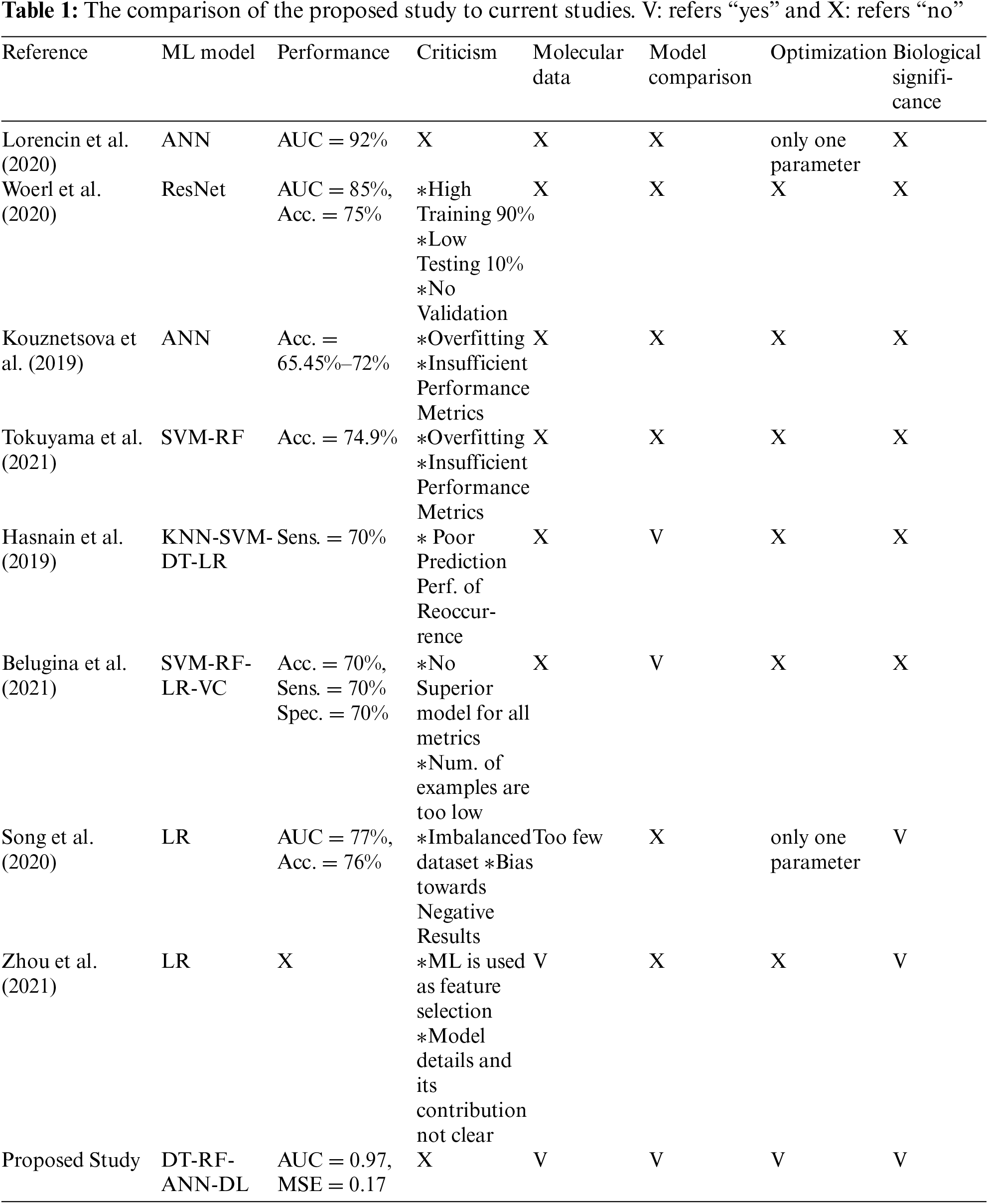
ML studies on BCa have significant shortcomings that are listed in Table 1. Based on these shortcomings, a study comparing different ML methods on molecular data is presented. In order to achieve the best performance of each model, hyper-parameter optimization was made. For each model, SNPs that affected the decision were extracted with an appropriate algorithm. The biological significance of the relevant SNPs was also examined.

3  Materials and Methods

The main aim of the study is given as follows:

•   To reveal variables that affect BCa with an appropriate method for the ML algorithm.

•   To compare the classification performance of the widely used ML models on the genomic data of BCa.

•   To optimize the hyper-parameters of each ML model.

•   To reveal the common SNPs and their biological significance.

Revealing SNPs that affect BCa could expand the genetic knowledge regarding the given disease. The newly discovered SNPs that affect BCa could be the starting point for future studies. Detection of BCa-causing SNPs can be used for the development of genetic kits to be used in the diagnosis of this disease and for the development of methods to be used in its prevention.

In order to achieve these aims a study design, given in Fig. 1, was conducted.

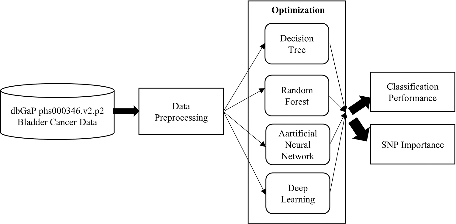
Figure 1: The overall structure of the process flow

The pre-processing phase is based on association analysis that reduces the number of related SNPs. Then, the sample dataset is given to the machine learning algorithms. Each algorithm, given in Fig. 1, enters the optimization step for hyper-parameter configuration. In this way, it is ensured that each algorithm gives the best performance. Then, the classification performances were compared in terms of MSE, RMSE and AUC. For each model, the SNPs that affect the classification were extracted and their effects on BCa were also discussed.

3.1 Materials

In this study, BCa was chosen as the disease because ML studies that used genetic information in BCa diagnosis are relatively less when compared to other cancer types. With this purpose, the dataset “Genome-wide association study for Bladder Cancer Risk” from database of genotypes and phenotypes (dbGaP) with accession number phs000346.v2.p2 was used. The most important reason for choosing this dataset was its open access. This way, different studies can use the same dataset. With its large and comprehensive structure, this dataset is suitable for ML use. In addition, it contains phenotype information as well as genomic data, and such datasets are extremely rare.

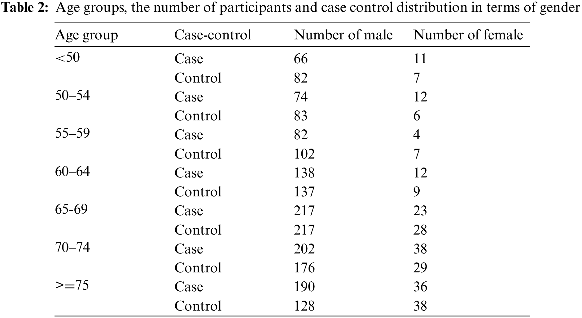
The molecular data platform was Human1Mv1_C. The raw datasets contained 1105 cases and 1049 controls with each having 591,637 SNPs. The case-control status, age and gender of the participants were provided as phenotypes. The dataset was divided as 60% train-test and 40% validation. The original case-control distribution was preserved in both sets. The validation set was not used in the training and testing phase. The performance scores and error metrics were calculated on the validation set. The age groups and the distribution of cases and controls in terms of gender are given in Table 2 below.

The dataset was analyzed for outliers and missing values, and none was found. In order to reduce the number of SNPs and to work on most related ones, an association analysis-based feature selection was conducted. PLINK [15] was used for this analysis. SNPs that met p < 0.001 were selected, which reduced the number of SNPs to 1334.

3.2 Methods

The literature review showed that the most preferred methods for genome wide association study (GWAS)-based medical diagnostic models were DT, RF, ANN and DL. In the following sub-sections, the details of the algorithms are given along with the optimization phase.

3.2.1 Decision Tree

DT, which is frequently preferred in classification problems, visually shows how the classification or prediction decision is made according to the attributes at hand. Tree structure shows the attributes that affect the result. The discrimination power of the attributes decreases from top to the bottom nodes.

Quinlan’s C4.5 [16] tree algorithm was used in our study. Entropy-based calculations were used to assign an attribute to a given node.

When the examples are denoted as Ei and the classes are denoted as Ci, the probability of the examples belonging to class Ci is given as Pi. In this case, information required to classify an attribute A that takes N values is given in Eq. (1).

E(A)=∑j=1nE1j+E2j+…+EnjE∗I(E1j,E2j,…,Enj)(1)

In this case, Eij represents the instances of Ej belonging to class Ci. Thus, the required information for Ej was calculated as in Eq. (2).

I(E1j,E2j,…,Enj)=−∑i=1npijlogpij(2)

Then the information gain of an attribute was calculated as in Eq. (3).

Information Gain=I(E1,E2,…En)−E(A)(3)

This calculation was used for all attributes, and the attribute with the highest information gain was assigned to the corresponding node of the tree.

In order to find the optimum hyper-parameters, the algorithm was given to an optimization phase. Splitting criteria, depth of the tree, minimum leaf size, and minimum size for split were the parameters used for optimization. The details of the optimization phase are given in the Section 3.2.5.

3.2.2 Random Forest

RFR RF is an ensemble of DTs [17]. Classification or prediction is made by majority voting. With this scheme, the overfitting problem of a single DT can be avoided [18].

In the tree construction phase, the dataset was randomly sampled in a bootstrapping manner, and it was used for training [19]. Then, the attributes were randomly selected, and each of them was tested to be assigned to a given node, as in DT [20].

In the DT approach, the importance of attributes can be determined by traversing the paths of the tree in a top down manner. However, since there are multiple trees in RF, attribute importance was determined by the Gini Significance [21] and by the probability of the attribute in a given node. The Gini significance is given in Eq. (4). In this equation, for a given node Ni, the importance of the node is denoted by IMPNi, the weighted number of samples in that node is Wi, the impurity is Ci, Ri is the right child, and Li is the left child.

IMPNi=WiCi−WLiCli−WRiCRj(4)

The importance of an attribute A in node Ni is given in Eq. (5).

IMPAi=∑iIMPNi∑jIMPNj(5)

This importance is calculated for all trees and then proportioned to the number of trees in the forest.

3.2.3 Artificial Neural Network

ANN is based on McCulloch and Pitts [22] and the perceptron [23] structure that mimics the human nerve cell. Each perceptron corresponds to a single neuron, and when these are arranged in layers (input-hidden-output layers), the network structure is formed. Each neuron evaluates inputs with a sum function along with their weights. The total input can be calculated by functions such as summation, multiplication, incremental summation, etc. The result from the summation function is given to the activation function to determine the output of the neuron. Linear, stepwise, and threshold functions are preferred in simple applications, while sigmoid, hyperbolic tangent (tanh), RELU or leaky RELU can be used for more complex problems [24].

When all neurons in the network are operated as described above, the prediction of the output layer is compared with the actual result. For this comparison, error metrics or loss functions can be used [25]. The weights are then adjusted until a predetermined error rate is reached.

In this study, the summation function was preferred. Different activations functions, sigmoid, tanh, and RELU versions were evaluated. Due to their value ranges, Sigmoid and Tanh functions have difficulty in converging the global minimum (gradient vanishing) [26]. Although this problem is partially solved with RELU function, RELU dying problem [27] occurs for min input values. To avoid such problems, Leaky RELU [28] was used in the related study.

The remaining hyper-parameters, such as learning rate, epoch and epsilon, were determined by the optimization phase.

3.2.4 Deep Learning

Deep networks are multi-layer neural networks with more hidden layers. DL models can be grouped under three main categories: deep networks, convolutional networks, and recurrent networks. The data in our study is not time dependent, and there is no need for down sampling. Thus, instead of recurrent or convolutional architectures, a fully connected deep neural network structure was preferred. In a fully connected deep neural network, the important parameters are activation function, regularization, loss, and the architecture.

The activation simply decides if a neuron will fire or not according to the sum of inputs and the added bias. Max Out activation was used in our study because they could learn any nonlinear function by piecewise linear function approximation [29].

Regularization schemes are used to prevent the model from overfitting. One approach is adding a penalty term to reduce the weights of neurons. For this purpose, L1 and L2 regularizations (Schmidt et al., 2007) can be used. However, they can introduce high variance [29,30]. In order to prevent that, drop out [31] strategy, in which randomly selected neurons are omitted, was used. The drop out ratio was determined by the optimization phase.

All ML models try to reduce the error of the approximation function. In DL structures, this error can be calculated via loss function [32]. The loss function is closely related to the given problem. In this study, the problem is binary classification; thus, logarithmic loss [33] was used.

It is very hard to calculate the variable importance in black box approaches. Garson [34], Goh [35], Olden et al. [36] and Gedeon [37] are widely used for this calculation.

The Gedeon method was preferred in our study because it was specifically designed for DL. The method calculates the variable importance based on the contributions of input nodes to outputs. Each input is evaluated by weight, by the similarity relations of the hidden layers nodes, and by the sensitivity analysis. The contribution of an input on an output Pjk, without weight cancellation of negative and positive weights, were calculated as in Eq. (6) [37].

Pjk=|Wjk|∑r=1nh|Wrk|(6)

Here, W denotes the weight; n is the number of nodes in the next layer; h is the number of nodes in the hidden layer; and j and k respond to the nodes in the jth and kth layers.

Vector similarity based on angular data can be used to identify the relationship between neurons in hidden layers [38]. The similarity angel between vectors can be calculated as in Eq. (7) where sact denotes the similarity of the activation functions.

angle(i,j)=tan−1⁡(∑ppatssact(p,i)2∑ppatssact(p,j)2∑ppats(sact(p,i)sact(p,j))2−1)(7)

The effect of input change on output can be determined by sensitivity analysis. This affect is based on the derivative change, as Eq. (8) [39] indicates.

dykdxi=dykdUk2.dUk2dhj.dhjdUj1.dUj1dxi(8)

3.2.5 Optimization Phase

In ML, fine-tuning of model parameters is the key factor for increasing performance [40]. Grid search, random search, and evolutionary search are widely used for this purpose [41].

The grid search approach tests all possible combinations for all hyper-parameters and their value ranges. It is a very effective method when the number of parameters and their value range is small [42]. When the number of parameters and value ranges increases, it becomes costly in terms of time and computational power [42].

The costs of the grid search can be reduced by random search [42]. In random search, pre-defined number of combinations, which are chosen randomly, are tested [43]. Although the optimization performance is quite high, there is a probability that the best parameter combinations could be overlooked depending on random selection ratio [44].

Evolutionary algorithms also narrow the search space by random selection. Even though the randomly selected combinations are not optimal, the new generations created by mutation and crossover converge to global optimum [43]. Thus, in general, they perform better than random search [45]. In addition, evolutionary hyper-parameter optimization (HPO) is proven to work superior on black box machine learners such as ANN and DL [46].

With its ability to converge to the global optimum and to reduce time and computational cost, an evolutionary HPO was used to optimize the C4.5, RF, ANN and DL models. In the HPO algorithm, Gaussian mutation with tournament selection with a fraction of 0.25 and cross over probability of 0.9 was used.

4  Results

In this section, the result of the HPO model is given first. Then, the classification performance of each model is given in terms of MSE, RMSE, and AUC. For each model, the related SNPs were revealed in order of importance and their biological significance was also investigated.

In this study, two ML approaches, the DT-based and black box-based approaches, were used. Because of the similarities of the hyper-parameters, the HPO results were arranged according to these main methods.

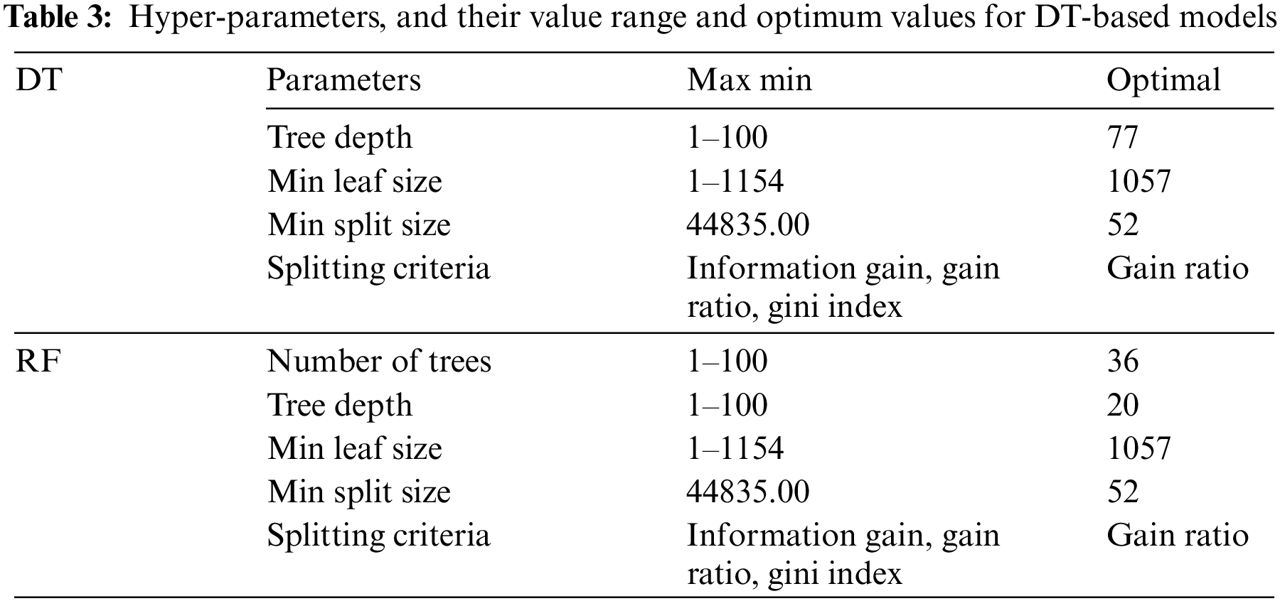
The DT-based methods share hyper-parameters such as splitting criteria, tree depth, minimum leaf size, and minimum split size. In addition to these parameters, the number of trees to be created must be set for RF. The learning algorithm, hyper-parameters, their value range, and optimum values are given in Table 3.

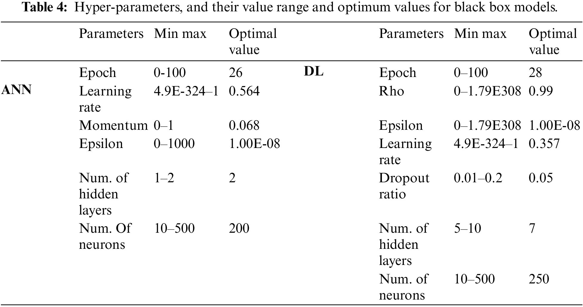
Black box algorithms share hyper-parameters such as epoch, learning rate, and epsilon. In addition to these, the DL model also has other hyper-parameters such as drop out ratio. The network architecture was also optimized in terms of hidden layers and number of neurons in hidden layers. Hyper-parameters, network architecture parameters, their value range, and optimum values for black box models are given in Table 4.

Each model was constructed by optimized hyper-parameters and then trained with 5-fold cross validation. The models were tested on a separate validation dataset. To compare the models, MSE and RMSE were used as error metrics, and Logloss was used as cost function. True positive and false positive rate is very crucial, especially for clinical applications [47]. Thus, AUC metric was used to show the relationship between these values.

For each model, the performance metrics given above were obtained for the training, testing and validation phases. The results of the validation phase and the effect of the hyper-parameter optimization over performance are given in Table 5.

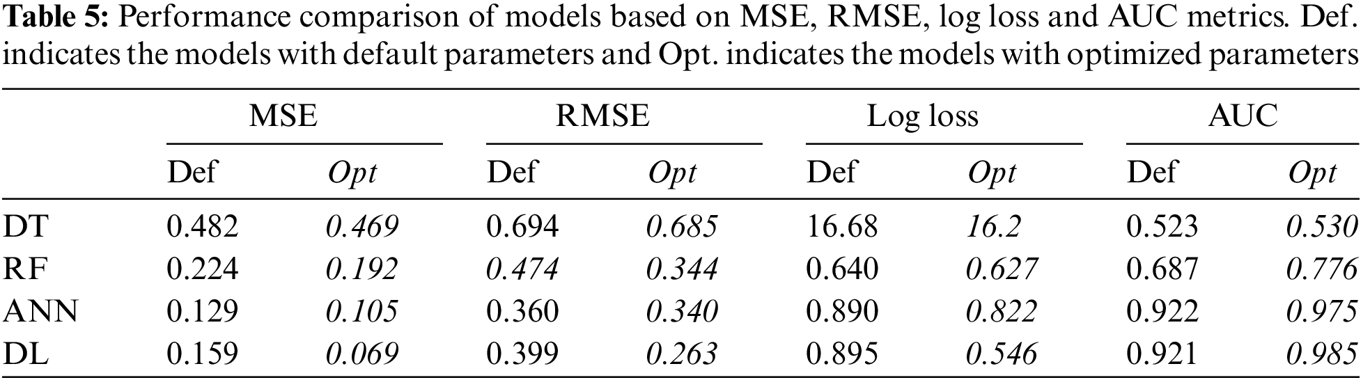
Table 5 indicates that DT performed poorly in terms of error, cost and AUC. AUC value of 0.530 shows that the DT model had an underfitting problem. The vast number of attributes can explain this poor performance. In addition, even if optimum parameters were used, a single tree may not be sufficient to show all possible splits. This situation is also known as the singularity problem of DT [48]. Proving this situation, RF showed a better classification performance than DT. The AUC values of the DT and RF models in the training and validation phases were compared to reveal the underfitting/overfitting status. The results are given in Fig. 2.

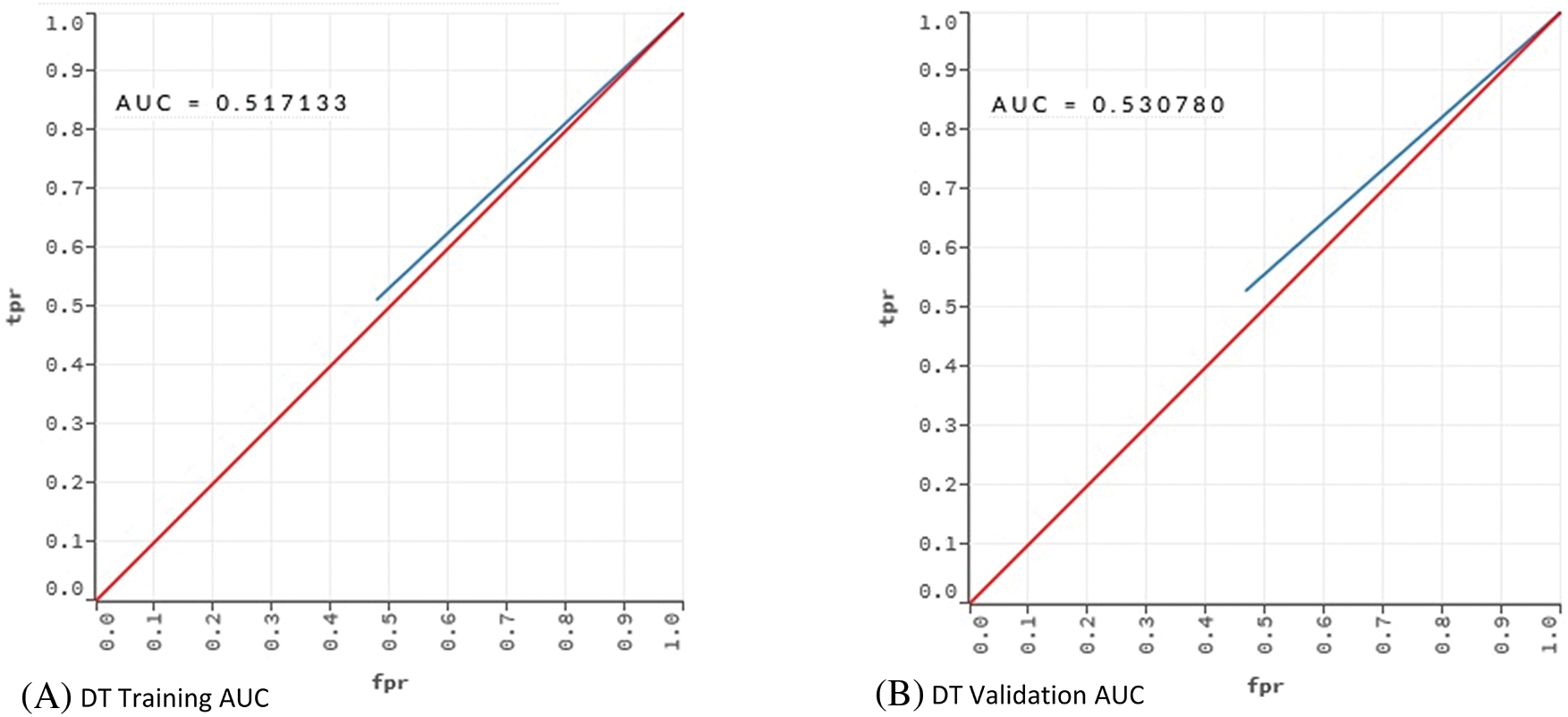
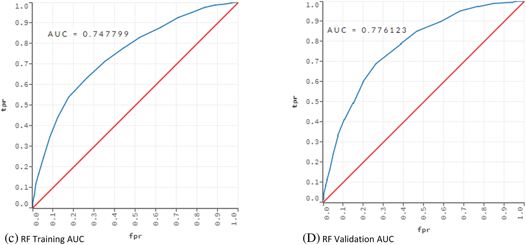
Figure 2: AUC values for training and validation of the models DT and RF

The training and validation comparison of the AUC value shows that there is an underfitting problem for DT. On the other hand, when the AUC values for RF are examined, no underfitting or overfitting is observed.

The two black box models outperformed the DT-based models. The performances of ANN and DL were almost similar. The AUC values for training and validation and their comparison are given in Fig. 3.

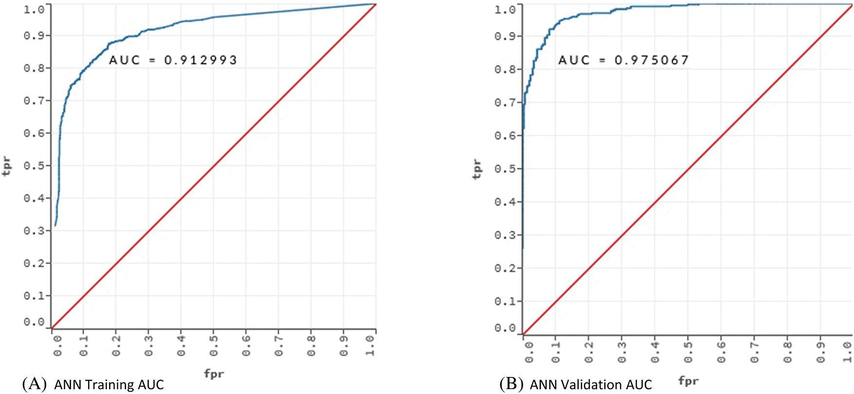
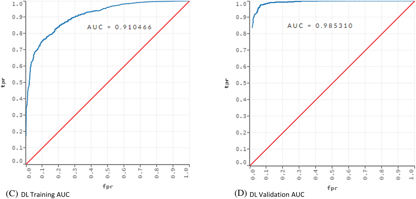
Figure 3: AUC values for training and validation of the models ANN and DL

Fig. 3 showed that the models learned the dataset without overfitting. For the ANN model, the training AUC was 0.92 and the validation AUC was 0.97. The AUC values for the training and validation of the DL model were 0.91 and 0.98, respectively.

The effect of the hyper-parameter optimization on the performance of each model was also investigated. For each metric, the ratio between default results and optimized results, given in Table 5, was calculated. For MSE, RMSE, and LogLoss error metrics, HPO had the best results over the DL model, with values of 57%, 17.5%, and 13%, respectively. When evaluated in terms of AUC, HPO made the best improvement on the RF model with an increase of 12%. HPO’s average increase over each performance metric was 30% for MSE, 17.5% for RMSE, 13% for LogLoss, and 6.75% for AUC.

The low increase in average AUC can be linked to very high and very low AUC values of the models. Since the AUC value for DT is 0.5, which indicates underfitting, the model’s failure to learn cannot be corrected by HPO alone. On the other hand, the AUC value for the black box models was quite high even when the default parameters were used. In this case, it is not expected that HPO will dramatically increase the AUC value which is already high. Since the AUC value to be increased with HPO for the black box models will approach the gold standard of 1, this may cause an overfitting problem. The effect of HPO on AUC can be revealed when AUC value is above 0.5 and below 0.9. As seen in Table 5, the AUC of the RF model was 0.687, and an increase of 12% was provided with HPO.

When evaluated as a whole, HPO seems to increase the performance. This increase was mostly observed on error metrics. It is very difficult to make a sound interpretation of HPO contribution in models where the AUC metric is very low (0.5 and below) or very high (0.9 and above). However, HPO has a potential to increase the performance of models that perform adequately in terms of AUC.

The SNPs found to affect BCa were listed for each model. These SNPs were ranked in order of importance. This ranking was based on the levels of the tree in the DT model. In the DT approach, the most discriminative attribute is calculated by information gain and assigned to the top node of the tree [16]. Thus, discriminative power of attributes in top layers are higher [16]. The discrimination power of the attributes in the same layer were accepted as equal. For the RF model, the variable importance were calculated based on Eqs. (4) and (5). Gedeon variable importance was used for the ANN and DL models. The top 20 SNPs ranked by variable importance for each model are given in Table 6.

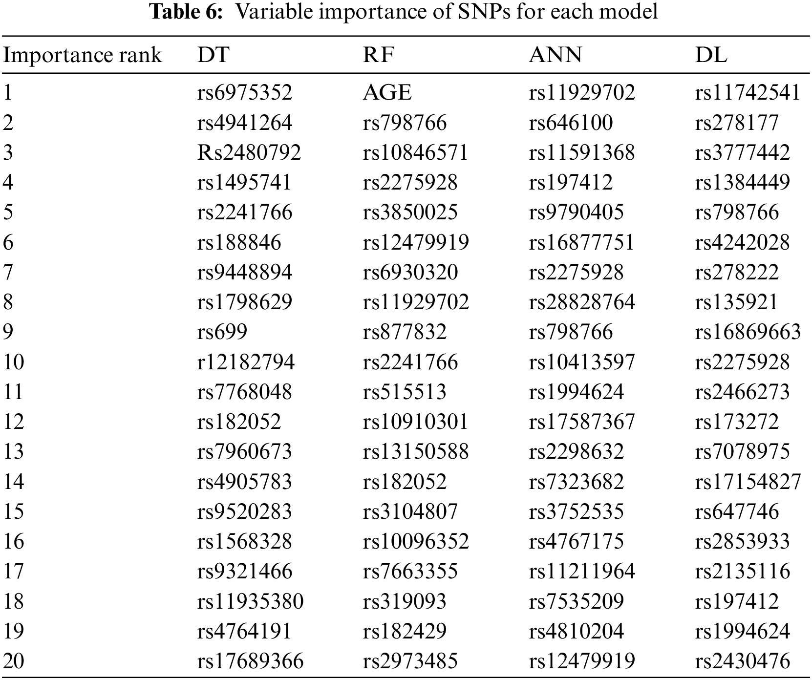
The top 20 SNPs revealed by each ML model are listed by importance order in Table 6 The highlighted SNPs in Table 6 indicate that the corresponding SNP was found to be important by more than one model. According to variable importance, the only phenotype attribute that affect the BCa is AGE. This attribute was found by the RF model. However, the other models did not find any phenotype attributes to be descriptive on the classification decision.

To reveal biological significance, the RegulomeDB [49] and SNPnexus [50] databases were used. RegulomeDB shows the regularity potential of the relevant SNP with a score table, even if it is in the non-coding region. The ranking and scores of the common SNPs retrieved from RegulomeDB are given in Table 7.

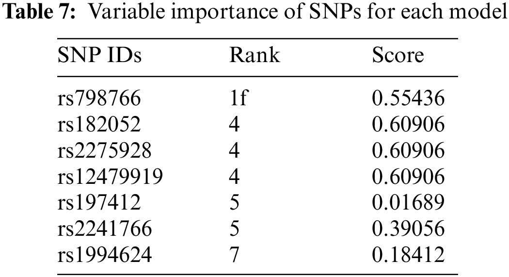
The SNPs were ranked from 1 to 7, with 1 being the most significant for binding and gene expression [51]. According to Table 7, rs798766 is highly associated with the BCa.

SNPnexus shows many interactions, such as gene/protein consequences, population data, regulatory elements, etc., according to the given genome information. In this study, SNPnexus was used to find the associations of the common SNPs and BCa. The disease SNP associations are given in Table 8.

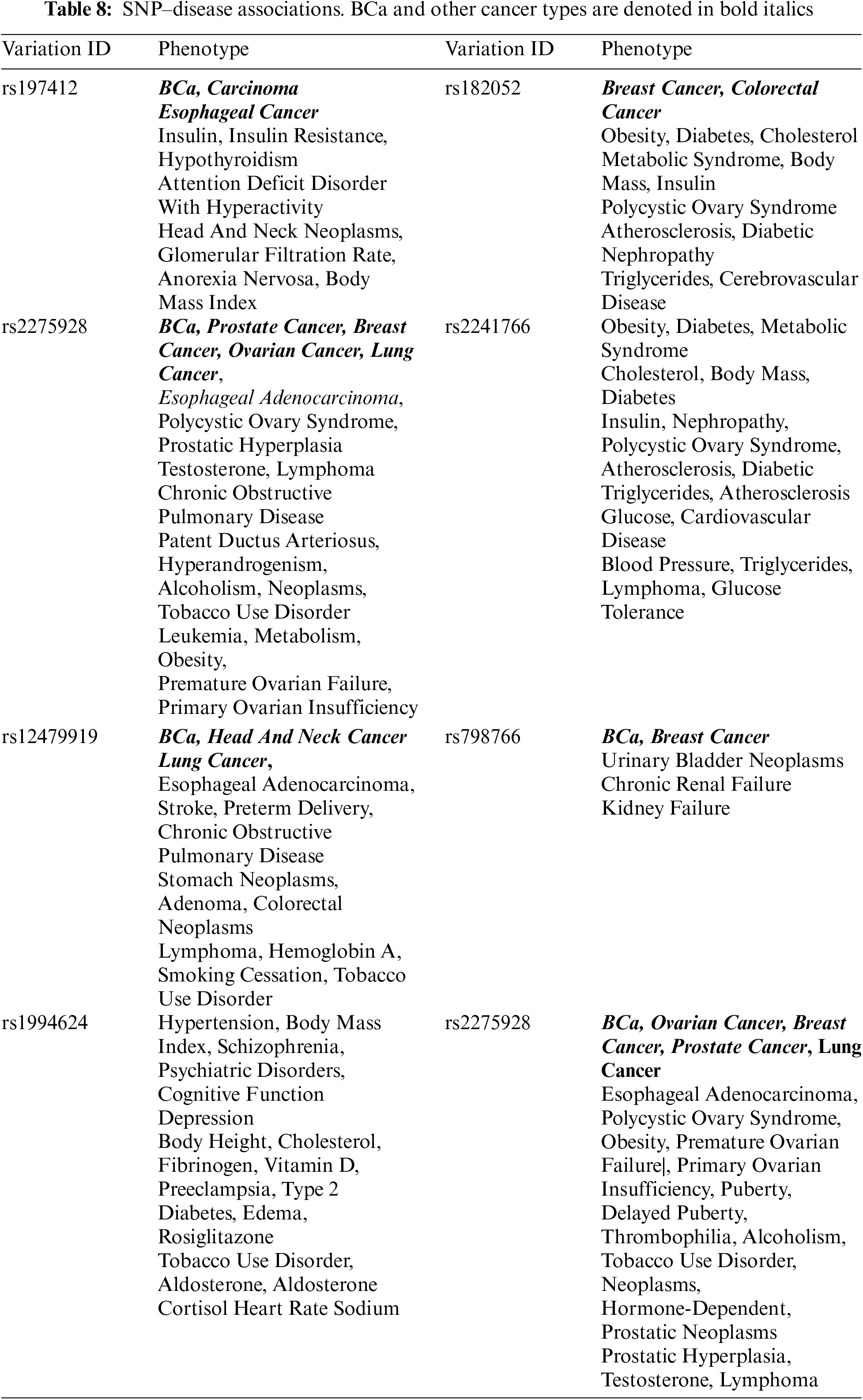
SNPnexus showed that five out of eight common SNPs were closely related with BCa. These SNPs were rs197412, rs2275928, rs12479919, rs798766, and rs2275928. The effect of these SNPs on BCa are also given in different studies. Golka et al. [51] stated that rs798766 was related to BCa. Likewise, the SNPs rs12479919, rs2275928 [52] and rs197412 were also found to be related to BCa [53]. The SNPs rs2241766 and rs182052 were found to be related to renal carcinoma [54]. Only two SNPs (rs1994624 and rs2241766) were not related to any cancer disease. However, these SNPs appear to be associated with conditions, which are known to cause cancer, such as tobacco and alcohol use, cholesterol, body mass index, diabetes, etc.

The results of the study, whose main motivation is to reveal genetic factors underlying BCa with different ML methods, are summarized in Fig. 4.

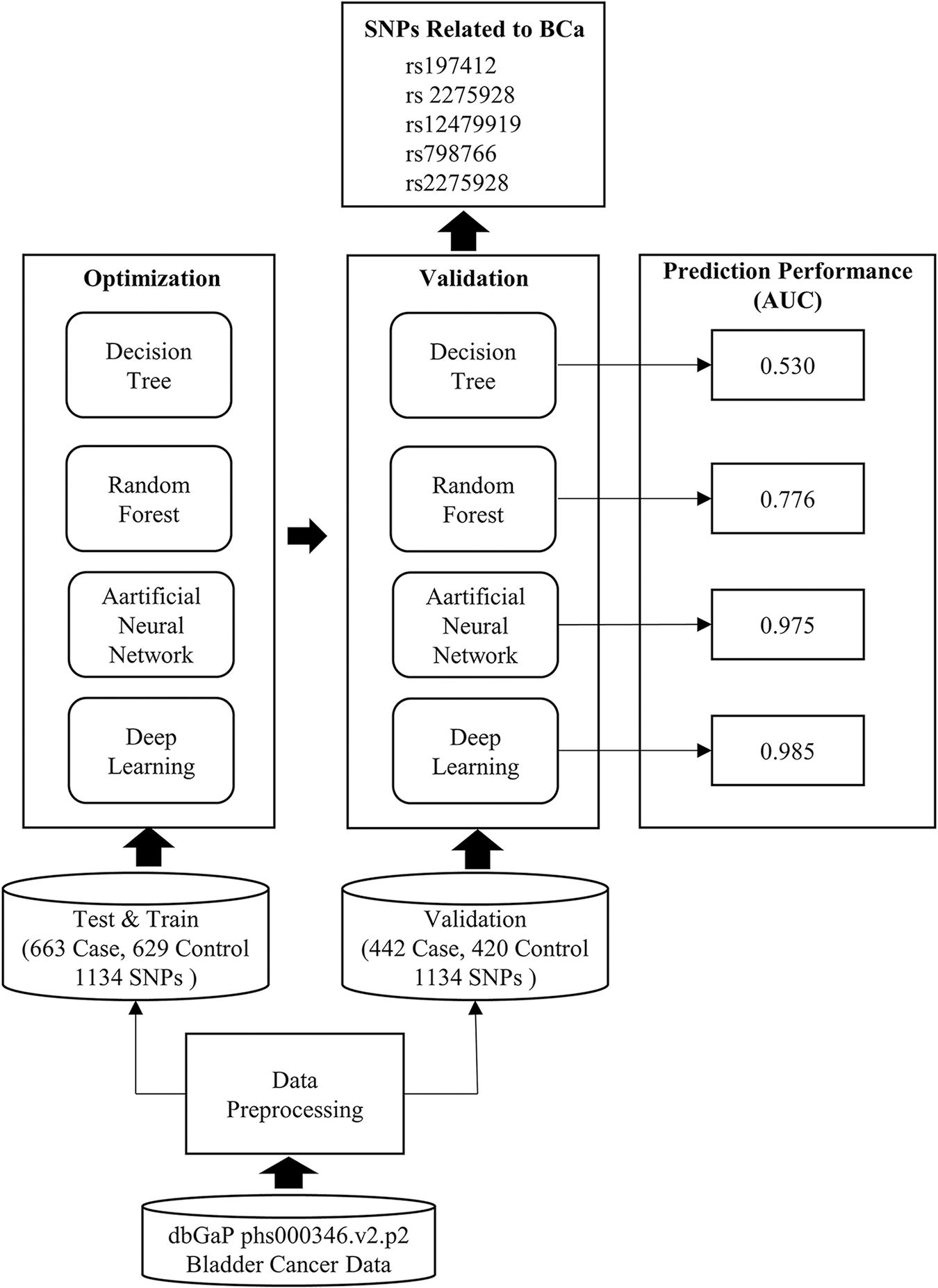
Figure 4: Workflow and obtained results of the study

The study started with the data-preprocessing phase. The original dataset was divided into 60% and 40% as train-test and validation. The case control ratio was kept equal in each dataset, and the samples were randomly assigned. The number of SNPs, which was 591,637 in the original dataset, was reduced to 1134. In the HPO phase, an evolutional algorithm with Gaussian mutation was used. The tournament selection ratio was set to 0.25, and crossover probability of 0.9 was used for each model. The ML methods were established with hyper-parameters obtained from HPO (Tables 3 and 4). Then, each model was run on the validation set. The performance and error metrics of each model are given in Table 5. The model with minimum error rate (MSE = 0.069) and the highest prediction performance was DL (AUC = 0.975). The SNPs causing BCa were extracted (Table 6) by using entropy, information gain and Gini index for the DT-based models and by using Gedeon importance for black box models. The biological significance of these SNPs was examined (Table 7). Five SNPs (rs197412, rs2275928, rs12479919, rs798766, rs2275928), which all models found to be important in common, were directly related to BCa. In addition, the other SNPs were found to be associated with cancer and cancer-causing conditions (Table 8). Two SNPs (rs1994624 and rs2241766) revealed by the models were suggested as susceptibility loci for BCa.

5  Conclusion

Machine learning algorithms are widely used in medical diagnosis. The use of these methods in genomic studies has become popular in recent years. However, there are some important shortcomings of current studies. The most important of these is not examining the factors that underlie predictions. In this case, a model can predict a given disease based on genomic data, but genetic causes will remain unknown. Another shortcoming of current studies is the lack of hyper-parameter optimization. ML studies on genomic data focus on prediction performance. However, they often do not optimize parameters that can increase the prediction performance. Based on these points, the motivation of our study was to reveal genetic factors causing BCa from different ML models and to provide a high prediction performance.

In this study, the models of two different main ML methods, which are frequently preferred in genetic datasets, were developed. To represent DTs, C4.5 and RF were used. ANN and DL were used to represent black box models. In order to establish the best prediction performance for each model, HPO was conducted. Different algorithms were used to reveal the SNPs that caused BCa for each model. While Gedeon variable importance was used for black box models, entropy and Gini index-based calculations were made for DTs.

The biggest limitation of the study was the scarcity of phenotype information in the dataset. ML studies on genetic data have difficulty in achieving a high prediction performance without phenotype data. The dataset used in this study includes only two phenotypes, age and gender. However, having phenotypes such as demographic information, blood test values, medical imaging results, etc. could improve prediction performance. The multidimensional and high amount of data consisting of only genetic factors can affect the performance negatively. Because most of the genetic data, in the form of SNPs, are not very strongly related to the disease at hand. To overcome this situation, various feature selection/elimination methods can be preferred. However, these methods may ignore biological significance in some cases. To prevent that, PLINK was used. In this way, biological significance was preserved while SNPs with low discrimination power were eliminated.

When evaluated on the basis of the ML method, DTs faced the singularity problem because of their branching strategy. High error and low prediction values for C4.5 prove this condition. RF consisting of alternative trees was used to solve the singularity problem of DT. Black box based-models are more performant in terms of prediction with their training strategy. However, the difficulty here is to reveal the variables that affect the result from the black box structure. The straightforward approach is to obtain weights in each layer of the neural network structure. However, weights alone are not sufficient to represent the significance of the variable. For this reason, the Gedeon variable importance, which uses similarity rates and sensitivity analysis as well as weights, was preferred.

The biggest limitation for HPO is the large number of parameters to be optimized for each different model. For example, in order to optimize C4.5 with four basic parameters by the value ranges given in Table 3, 6,655 combinations must be used. Similarly, over 100,000 combinations were needed to optimize the DL parameters. This leads to computational and time cost. To reduce these costs, similar studies search the combination space with random search. However, this approach increases the possibility of missing the best parameter combination. In this work, an evolutionary search approach was used to find the best combination of parameters while reducing computational and time cost.

In this study, four different ML models were used to reveal genetic features of BCa. These models were compared in terms of error metrics and prediction performance. The biological significance of these features was also tested. Among the models, DL was superior in terms of error metrics (MSE = 0.069, RMSE = 0.263, Logloss = 0.546) and prediction performance (AUC = 0.985). The biological significance of the SNPs, found by each ML model, was investigated using the RegulomeDB and SNPnexus databases. Five of the common SNPs (rs197412, rs2275928, rs12479919, rs798766 and rs2275928) were closely associated with BCa. The relationship of these SNPs with BCa was also shown in different studies in the literature [51–54]. In addition, two new susceptibility loci (rs1994624 and rs2241766) were revealed for further genomic investigations in the future.

In the medical field, finding the factors that cause the disease is as important as the diagnosis. When evaluated in this context, this study successfully found the factors associated with BCa and also suggested two different SNPs whose relationship with BCa was not known before. With future studies on these SNPs, genetic factors causing BCa can be expanded. When causative or protective factors are known, genetic test kits can diagnose individuals before they become ill. With preventive medicine, the number of current patients can be significantly reduced. The biological results obtained in our study have the potential to help in the development of these genetic test kits.

In terms of ML, our study has the potential to guide the use of DT and black box models on genetic data. It can also guide future studies for HPO optimization. Our plan for this study was shaped around two points. The first of these was to establish an ensemble model instead of a single one whereas the other was to further refine the evolutionary algorithm for the hyper-parameters of the ensemble model. It was set as a future study target to optimize the evolutionary algorithm within itself and to ensure the highest performance of the ensemble model.

Acknowledgement: The data/analyses presented in the current publication were based on the use of the study data downloaded from the dbGaP web site, under phs000346.v2.p2.

N. Rothman, M. Garcia-Closas, N. Chatterjee, N. Malats and X. Wu et al., “A multi-stage genome-wide association study of bladder cancer identifies multiple susceptibility loci,” Nature Genetics, vol. 42, no. 11, pp. 978–984, 2010.

M. Garcia-Closas,Y. Ye,N. Rothman, J. D. Figueroa and N. Malats et al., “A genome-wide association study of bladder cancer identifies a new susceptibility locus within SLC14A1, a urea transporter gene on chromosome 18q12.3,” Human Molecular Genetics, vol. 20, no. 21, pp. 4282–4289, 2011.

J. D. Figueroa, Y. Ye, A. Siddiq, M. Garcia-Closas and N. Chatterjee et al., “Genome-wide association study identifies multiple loci associated with bladder cancer risk,” Human Molecular Genetics, vol. 23, no. 5, pp. 1387–1389, 2014.

Funding Statement: The author received no specific funding for this study.

Conflicts of Interest: The author declares that he has no conflicts of interest to report regarding the present study.

References

1. A. S. Ahuja, “The impact of artificial intelligence in medicine on the future role of the physician,” PeerJ, vol. 7, no. 2, pp. e7702, 2019. [Google Scholar] [PubMed]

2. M. Libbrecht and W. Noble, “Machine learning applications in genetics and genomics,” Nature Reviews Genetics, vol. 16, no. 6, pp. 321–332, 2015. [Google Scholar] [PubMed]

3. I. J. Bergerød, G. S. Braut and S. Wiig, “Resilience from a stakeholder perspective: The role of next of kin in cancer care,” Journal of Patient Safety, vol. 16, no. 3, pp. e205–e210, 2020. [Google Scholar]

4. K. A. Tran, O. Kondrashova, A. Bradley, E. D. Williams, J. V. Pearson et al., “Deep learning in cancer diagnosis, prognosis and treatment selection,” Genome Medicine, vol. 13, no. 1, pp. 152, 2021. [Google Scholar] [PubMed]

5. T. D. Gedeon, “Data mining of inputs: Analysing magnitude and functional measures,” International Journal of Neural Systems, vol. 8, no. 2, pp. 209–218, 1997. [Google Scholar] [PubMed]

6. R. S. Ibarrola, S. Hein, G. Reis, C. Gratzke and A. Miernik, “Current and future applications of machine and deep learning in urology: A review of the literature on urolithiasis, renal cell carcinoma, and bladder and prostate cancer,” World Journal of Urology, vol. 38, no. 10, pp. 2329–2347, 2020. [Google Scholar]

7. I. Lorencin, N. Anđelić, J. Španjol and Z. Car, “Using multi-layer perceptron with Laplacian edge detector for bladder cancer diagnosis,” Artificial Intelligence in Medicine, vol. 102, no. 1, pp. 101746, 2020. [Google Scholar] [PubMed]

8. A. C. Woerl, M. Eckstein, J. Geiger, D. C. Wagner, T. Daher et al., “Deep learning predicts molecular subtype of muscle-invasive bladder cancer from conventional histopathological slides,” European Urology, vol. 78, no. 2, pp. 256–264, 2020. [Google Scholar] [PubMed]

9. V. L. Kouznetsova, E. Kim, E. L. Romm, A. Zhu and I. F. Tsigeln, “Recognition of early and late stages of bladder cancer using metabolites and machine learning,” Metabolomics, vol. 15, no. 7, pp. 94, 2019. [Google Scholar] [PubMed]

10. N. Tokuyama, A. Saito, R. Muraoka, S. Matsubara, T. Hashimoto et al., “Prediction of non-muscle invasive bladder cancer recurrence using machine learning of quantitative nuclear features,” Modern Pathology, vol. 35, no. 4, pp. 533–538, 2021. [Google Scholar] [PubMed]

11. Z. Hasnain, J. Mason, K. Gill, G. Miranda, I. S. Gill et al., “Machine learning models for predicting post-cystectomy recurrence and survival in bladder cancer patients,” PLoS One, vol. 14, no. 2, pp. e0210976, 2019. [Google Scholar] [PubMed]

12. R. Belugina, E. Karpushchenko, A. Sleptsov, V. Protoshchak, A. Legin et al., “Developing non-invasive bladder cancer screening methodology through potentiometric multisensor urine analysis,” Talanta, vol. 234, no. 3, pp. 122696, 2021. [Google Scholar] [PubMed]

13. Q. Song, J. D. Seigne, A. R. Schned, K. T. Kelsey, M. R. Karagas et al., “A machine learning approach for long-term prognosis of bladder cancer based on clinical and molecular features,” in Proc. of AMIA Joint Summits on Translational Science, Houston, Texas, USA, pp. 607–616, 2020. [Google Scholar]

14. M. Zhou, Z. Zhang, S. Bao, P. Hou, C. Yan et al., “Computational recognition of lncRNA signature of tumor-infiltrating b-lymphocytes with potential implications in prognosis and immunotherapy of bladder cancer,” Briefings in Bioinformatics, vol. 22, no. 3, pp. bbaa047, 2021. [Google Scholar] [PubMed]

15. S. Purcell, B. Neale, K. Todd-Brown, L. Thomas, M. A. R. Ferreira et al., “PLINK: A toolset for whole-genome association and population-based linkage analysis,” American Journal of Human Genetics, vol. 81, no. 3, pp. 559–575, 2007. [Google Scholar] [PubMed]

16. J. R. Quinlan, “Learning decision tree classifiers,” ACM Computing Surveys, vol. 28, no. 1, pp. 71–72, 1996. [Google Scholar]

17. A. B. Shaik and S. Srinivasan, “A brief survey on random forest ensembles in classification model,” in Proc. of Int. Conf. on Innovative Computing and Communications, Gnim, New Delhi, India, pp. 253–260, 2018. [Google Scholar]

18. M. Bramer, “Avoiding overfitting of decision trees,” in Principles of Data Mining, 2nd edition, Newyork, USA: Springer Press, pp. 119–134, 2007. [Google Scholar]

19. Y. Qi, “Random forest for bioinformatics,” in Ensemble Machine Learning, 1st edition, Boston, MA, USA: Springer Press, pp. 307–323, 2012. [Google Scholar]

20. V. Y. Kulkarni and P. K. Sinha, “Pruning of random forest classifiers: A survey and future directions,” in Proc. of 2012 Int. Conf. on Data Science and Engineering, Cochin, India, pp. 64–68, 2012. [Google Scholar]

21. B. H. Menze, B. M. Kelm, R. Masuch, U. Himmelreich, P. Bachert et al., “A comparison of random forest and its Gini importance with standard chemometric methods for the feature selection and classification of spectral data,” BMC Bioinformatics, vol. 10, no. 213, pp. 1–16, 2009. [Google Scholar]

22. W. S. McCulloch and W. Pitts, “A logical calculus of the ideas immanent in nervous activity,” Bulletin of Mathematical Biology, vol. 52, no. 1–2, pp. 99–115, 1990. [Google Scholar] [PubMed]

23. F. Rosenblatt, “The perceptron: A probabilistic model for information storage and organization in the brain,” Psychological Review, vol. 65, no. 6, pp. 386–408, 1958. [Google Scholar] [PubMed]

24. A. K. Dubey and V. Jain, “Comparative study of convolution neural network’s relu and leaky-relu activation functions,” in Applications of Computing, Automation and Wireless Systems in Electrical Engineering, 1st edition, Singapore: Springer Press, pp. 873–880, 2018. [Google Scholar]

25. O. I. Abiodun, A. Jantan, A. E. Omolara, K. V. Dada, N. A. Mohamed et al., “State-of-the-art in artificial neural network applications: A survey,” Heliyon, vol. 4, no. 11, pp. e00938, 2018. [Google Scholar] [PubMed]

26. S. Basodi, C. Ji, H. Zhang and Y. Pan, “Gradient amplification: An efficient way to train deep neural networks,” Big Data Mining and Analytics, vol. 3, no. 3, pp. 196–207, 2020. [Google Scholar]

27. Z. Hu, J. Zhang and Y. Ge, “Handling vanishing gradient problem using artificial derivative,” IEEE Access, vol. 9, pp. 22371–22377, 2021. [Google Scholar]

28. A. L. Maas, A. Y. Hannun and A. Y. Ng, “Rectifier nonlinearities improve neural network acoustic models,” in Proc. of 30th Int. Conf. on Machine Learning, Atlanta, GA, USA, pp. 3, 2013. [Google Scholar]

29. I. Goodfellow, Y. Bengio and A. Courville, “Deep Learning,” in Adaptive Computation and Machine Learning Series. London, England: MIT Press, pp. 163–359, 2018. [Google Scholar]

30. C. Garbin, X. Zhu and O. Marques, “Dropout vs. batch normalization: An empirical study of their impact to deep learning,” Multimedia Tools and Applications, vol. 79, no. 19–20, pp. 12777–12815, 2020. [Google Scholar]

31. N. Srivastava, G. E. Hinton, A. Krizhevsky, I. Sutskever and R. Salakhutdinov, “Dropout: A simple way to prevent neural networks from overfitting,” Journal of Machine Learning Research, vol. 15, no. 1, pp. 1929–1958, 2014. [Google Scholar]

32. Y. Ho and S. Wookey, “The real-world-weight cross-entropy loss function: Modeling the costs of mislabeling,” IEEE Access, vol. 8, pp. 4806–4813, 2020. [Google Scholar]

33. Q. Wang, Y. Ma, K. Zhao and Y. Tian, “A comprehensive survey of loss functions in machine learning,” Annals of Data Science, vol. 9, no. 2, pp. 187–212, 2020. [Google Scholar]

34. D. G. Garson, “Interpreting neural-network connection weights,” Artificial Intelligence Expert, vol. 6, no. 4, pp. 46–51, 1991. [Google Scholar]

35. A. Goh, “Back-propagation neural networks for modeling complex systems,” Artificial Intelligence in Engineering, vol. 9, no. 3, pp. 143–215, 1995. [Google Scholar]

36. J. D. Olden, M. K. Joy and R. G. Death, “An accurate comparison of methods for quantifying variable importance in artificial neural networks using simulated data,” Ecological Modelling, vol. 178, no. 3, pp. 389–397, 2004. [Google Scholar]

37. T. D. Gedeon and D. Harris, “Network reduction techniques,” in Proc. of Int. Conf. on Neural Networks Methodologies and Applications, San Diego, USA, pp. 119–126, 1991. [Google Scholar]

38. A. Kabani and M. R. El-Sakka, “Object detection and localization using deep convolutional networks with softmax activation and multi-class log loss,” in Proc. Int. Conf. on Image Analysis and Recognition, Póvoa de Varzim, Portugal, pp. 358–366, 2016. [Google Scholar]

39. W. Liu, Z. Wang, X. Liu, N. Zeng, Y. Liu et al., “A survey of deep neural network architectures and their applications,” Neurocomputing, vol. 234, no. 4, pp. 11–26, 2016. [Google Scholar]

40. L. Hertel, J. Collado, P. Sadowski, J. Ott and P. Baldi, “Sherpa: Robust hyperparameter optimization for machine learning,” SoftwareX, vol. 12, no. 81, pp. 100591, 2020. [Google Scholar]

41. M. Feurer and F. Hutter, Hyperparameter optimization. In: Automated Machine Learning: Methods, Sysytems, Challanges. USA: Springer Cham, pp. 3–33, 2019. [Google Scholar]

42. Y. J. Yoo, “Hyperparameter optimization of deep neural network using univariate dynamic encoding algorithm for searches,” Knowledge-Based Systems, vol. 178, no. C, pp. 74–83, 2019. [Google Scholar]

43. L. Yang and A. Shami, “On hyperparameter optimization of machine learning algorithms: Theory and practice,” Neurocomputing, vol. 415, no. 1, pp. 295–316, 2020. [Google Scholar]

44. J. Bergstra and Y. Bengio, “Random search for hyper-parameter optimization,” Journal of Machine Learning Research, vol. 13, no. 2, pp. 281–305, 2012. [Google Scholar]

45. M. Stang, C. Meier, V. Rau and E. Sax, “An evolutionary approach to hyper-parameter optimization of neural networks,” in Proc. of Human Interaction and Emerging Technologies, Nice, France, pp. 713–718, 2019. [Google Scholar]

46. J. Bergstra, R. Bardenet, Y. Bengio and B. Kégl, “Algorithms for hyper-parameter optimization,” in Proc. of 24th Int. Conf. on Neural Information Processing Systems, Granada, Spain, pp. 2546–2554, 2011. [Google Scholar]

47. D. van Ravenzwaaij and J. Ioannidis, “True and false positive rates for different criteria of evaluating statistical evidence from clinical trials,” BMC Medical Research Methodology, vol. 19, no. 1, pp. 1–10, 2019. [Google Scholar]

48. M. Czajkowski and M. Kretowski, “Decision tree underfitting in mining of gene expression data. An evolutionary multi-test tree approach,” Expert Systems with Applications, vol. 137, no. C, pp. 392–404, 2019. [Google Scholar]

49. A. P. Boyle, E. L. Hong, M. Hariharan, Y. Cheng, M. A. Schaub et al., “Annotation of functional variation in personal genomes using RegulomeDB,” Genome Research, vol. 22, no. 9, pp. 1790–1797, 2012. [Google Scholar] [PubMed]

50. J. Oscanoa, L. Sivapalan, E. Gadaleta, A. Z. D. Ullah and N. R ., Lemoine et al., “SNPnexus: A web server for functional annotation of human genome sequence variation,” Nucleic Acids Research, vol. 48, no. W1, pp. W185–W192, 2020. [Google Scholar] [PubMed]

51. K. Golka, S. Selinski, M. L. Lehmann, M. Blaszkewicz, R. Marchan et al., “Genetic variants in urinary bladder cancer: Collective power of the wimp SNPs,” Archives of Toxicology, vol. 85, no. 6, pp. 539–554, 2011. [Google Scholar] [PubMed]

52. A. S. Andrew, J. Gui, A. C. Sanderson, R. A. Mason, E. V. Morlock et al., “Bladder cancer SNP panel predicts susceptibility and survival,” Human Genetics, vol. 125, no. 5, pp. 527–539, 2009. [Google Scholar] [PubMed]

53. A. J. Grotenhuis, A. M. Dudek, G. W. Verhaegh, J. A. Witjes, K. K. Aben et al., “Prognostic relevance of urinary bladder cancer susceptibility loci,” PLoS One, vol. 9, no. 2, pp. e89164, 2014. [Google Scholar] [PubMed]

54. Y. M. Hsueh, W. J. Chen, Y. C. Lin, C. Y. Huang, H. S. Shiue et al., “Adiponectin gene polymorphisms and obesity increase the susceptibility to arsenic-related renal cell carcinoma,” Toxicology and Applied Pharmacology, vol. 350, pp. 11–20, 2018. [Google Scholar] [PubMed]