Leaky Cable Fixture Detection in Railway Tunnel Based on RW DCGAN and Compressed GS-YOLOv5

1  Introduction

With the popularization of high-speed trains in daily life, the importance of related mobile communication systems has become increasingly prominent. In order to ensure that the train can communicate with outside normally in the railway tunnel, the full coverage of the Global System for Mobile Communications-Railway (GSM-R) signal is significant. At present, the leaky cable is mainly used to construct the communication network, and is fixed on the tunnel wall with special fixtures [1]. However, leaky cable fixtures are vulnerable to air pressure and power waves generated when high-speed trains pass through the tunnels. At the same time, the humid tunnel geological environment will also accelerate the loosening or even detachment of cable fixtures. Currently, the primary method of cable fixture detection is still manual periodic inspection. Obviously, it requires onsite manual working, which is not only inefficient but also has serious safety hazards. With the increasing mileage of railway tunnels, it is challenging to meet the actual needs only by manual detection.

Due to the development of computer vision algorithm, intelligent detection has been widely used in the security protection field of railway tunnels. Such as tunnel surface detection [2,3], rail surface detection [4–6], and crack detection of tunnel walls [7]. For leaky cable fixture detection, the general process has the following three steps: 1) The Special COMS dual-line camera is used to extract original image data sets, and these images also need to be processed to meet the detection requirements. 2) Use the corresponding feature extraction algorithm to obtain the fixture features, and put them into the machine learning classifier for training. 3) The trained classifier will detect testing data sets, and then the faulty samples will be identified. The vision-based method further improves the detection efficiency, greatly optimizes the working environment, and becomes the developing trend of leaky cable fixture detection.

Based on large-scale datasets, deep learning has achieved remarkable fault detection success. Monocular vision’s anchor-based detection algorithm is mainly divided into two-stage and one-stage modes. For example, Zhang et al. [8] proposed an enhancement Single Shot Multi-Box Detector (SSD) algorithm for leaky cable fixtures detection. They first used a pyramid structure to obtain the multi-scale features and then combined the inception structure and residual structure to improve network performance. Although the average accuracy of the model used in literature 6 is 90.4%, it is only 22 fps, which is challenging to meet the requirements of fixture detection. In order to improve detection speed, Ma [9] improved YOLOv4 and adopted Mobile-Net as backbone to extract cable fixture features. The accuracy of model in literature 7 is as high as 95.33%, but its data and quantity are small, and the model’s generalization is poor. Due to practical engineering constraints, obtaining annotated samples that fully satisfy the volume of training data set in leaky cable fixture detection is laborious or even impractical. Zhang et al. [10] proposed a multi-scale continuous gradient local binary pattern based on a manual handicraft algorithm to detect faulty fixtures. The accuracy of literature 8 reached 83.5%, but the traditional method is more dependent on the dataset and has a smaller number of datasets, making it less applicable. Peng [11] followed a two-stage method. They first used Snake to locate leaky cable fixtures and then operated Haar to extract characteristics. Although these manual algorithms can reduce the dependence on data sets, their portability and detection speed are poor. The main contributions of our work are highlighted as follows:

■   To address the overfitting phenomenon caused by traditional data enhancement methods with a single transformation and the problem of unstable GAN training, we propose the RW-DCGAN model. The model is used to implement data enhancement, enabling defective fixtures to output more high-quality and irregular images.

■   In order to improve the inspection speed of the clamps while maintaining accuracy, the GS-YOLOv5 model was proposed to meet the practical needs of tunnel leak detection.

■   To further improve the detection speed and to verify the validity of the model, we used a model compression strategy to trim redundant channels and used Grad-CAM to visualise the training details to verify the reliability of our method.

2  Related Work

For fault detection in the engineering field, the end-to-end detection algorithm based on one-stage has a faster speed, but its accuracy is lower. Although the two-stage algorithm can obtain higher accuracy, its lower speed is difficult to meet the needs of real-time detection. Therefore, the indicators to measure the leaky cable fixture detection algorithm need to be determined according to the actual situation. Similar problems also exist in boundary detection [12], bearing inspection [13], bridge crack detection [14], and machine fault diagnosis [15]. Many factors affect the model detection speed and detection accuracy. On the one hand, the ability of the model to acquire target features needs to be improved. The most common method is to enhance the comprehensive properties of the network model. However, it will inevitably increase the number of parameters and reduce computational efficiency, making it challenging to deploy in practical applications. On the other hand, a sufficient sample size is essential for a good model. But in most cases, the sample size is usually insufficient, so overfitting can also seriously affect the judgment of model detection performance.

2.1 Methods to Improve Detection Accuracy

The detection accuracy of the network is the most critical evaluation criterion, so many of the current researches are based on further improving detection accuracy. The most common way is to upgrade the network structure, to enhance the model’s ability to obtain target features. For example, Xu et al. [16] used the feature fusion method to construct multi-scale detection layers to improve detection performance. Kim [17] proposed an efficient channel attention pyramid YOLO to optimize the detection for small objects and improve detection accuracy by optimizing the detection layer to isolate other objects. Cai et al. [18] designed a new feature fusion PAN++ module and used five scale detection layers to capture small target objects. Li et al. [19] presented the electronic component detection network through effective receptive field size and anchor size matching in YOLOv3, which can realize the calculation and visualization of the effective receptive field size of different depth layers based on CNN gradient backpropagation. The above algorithm effectively improves detection accuracy, but their network structures are relatively complex. Besides, the large model size caused by the feature fusion method will seriously affect the detection speed.

2.2 Methods to Improve Detection Speed

The detection speed is also an important reference indicator for judging whether the model can be successfully deployed on mobile devices. Especially for some fields that need real-time detection, the results of time-out detection will lose their value. Howard et al. [20] use deep separable convolution to build a lightweight network instead of traditional convolution, which can improve the computational speed by reducing the amounts of parameters of the model. Zeng et al. [21] proposed a jump-join repetitious learning structure to detect dangerous objects and dangerous actions, which can accelerate the speed of feature extraction while integrating features of different scales. Zhang et al. [22] used packet convolutions and channel shuffling to build a lightweight network ShuffleNet that can be embedded in mobile terminals to reduce the computational load of the detection network further. In order to remove a large number of redundant features in the convolutional layers, Han et al. [23] proposed the Ghost module, which can remove redundancy through linear transformation, identity mapping, and other methods. Furthermore, it effectively reduces the computational complexity and increases the speed of the model. Although the lightweight network model has the advantages of fewer parameters and faster calculation speed, the accuracy is not high, and it is still difficult to meet the requirements of leaky cable fixture detection.

2.3 Methods to Data Augmentation

Deep learning is essentially a sample-based statistical learning algorithm, so the number of samples in the dataset is significant for the network model. To solve the problem of insufficient data samples, the most common method is to perform edge enhancement, image rotating, contrast enhancement, and other operations on the existing data. Although such a linear method increases the sample size and meets the requirements of model training, the regular transformation of the original image can easily lead to overfitting of the network model. In order to enrich the image and improve the detection quality of the model, the generic adversarial network (GAN) enhances the representation of images by competing and learning with each other in the generator and discriminator during training [24]. The generator and discriminator of DCGAN adopt CNN to replace the full connection network, eliminate the pooling layers, and use Leaky Relu and Sigmoid as the activation function, which can speed up model training and improve training stability [25]. Chen et al. [26] proposed a bidirectional generative adversarial framework, which adds global features to the network and uses the adaptive weighting scheme for training to improve model stability. Ni et al. [27] adopted embedded modulation and attention mechanisms to capture richer global and local features, and then combined fidelity loss and quality loss to preserve the desired characteristics. Liu et al. [28] introduced fractional order differentiation into generator and discriminator, which can better distinguish noise and high-frequency details. Although many networks have made progress in data augmentation, it still does not handle fixture images well. The main reason is that the size of the fixture image is relatively large, and it is hard to capture the fixture features accurately. Therefore, enhancing the expressive effect of fixture images can also further improve the detection performance.

3  The Proposed Method

The method proposed in this paper mainly improves the detection accuracy and detection speed of leaky cable fixtures. In order to meet the training requirements of our model, we first need to augment the fixture data to obtain more high-quality fixture images. Then use an improved feature extraction network to obtain fixture features and adopt a compression strategy to simplify our model and complete the entire detection work.

3.1 RW-DCGAN Model

3.1.1 Structure of RW-DCGAN

Due to the limitation of the number of layers in the network, most models are difficult to adapt to large-size images. Even if there is an image output, the fitting effect of the image is not good, and it is difficult to meet the training requirements. Therefore, this paper proposes the RW-DCGAN model, which enhances the ability to capture fixture features and can fit the 512 × 512 fixture images to meet the detection requirements. As shown in Fig. 1, the generator reshapes the input noise vector with dimension 100 into a feature map of size 4 × 4 × 1024. Then perform 7 times generator residual module processing and one convolution processing to obtain the fixture image with 512 × 512 × 3. The discriminator performs one convolution and 6 times discriminator residual module processing on the real or generated fixture image, and finally expands the feature into a one-dimensional output through the full connection layer. In order to avoid overfitting, the Dropout layer is also added at the end of the discriminator.

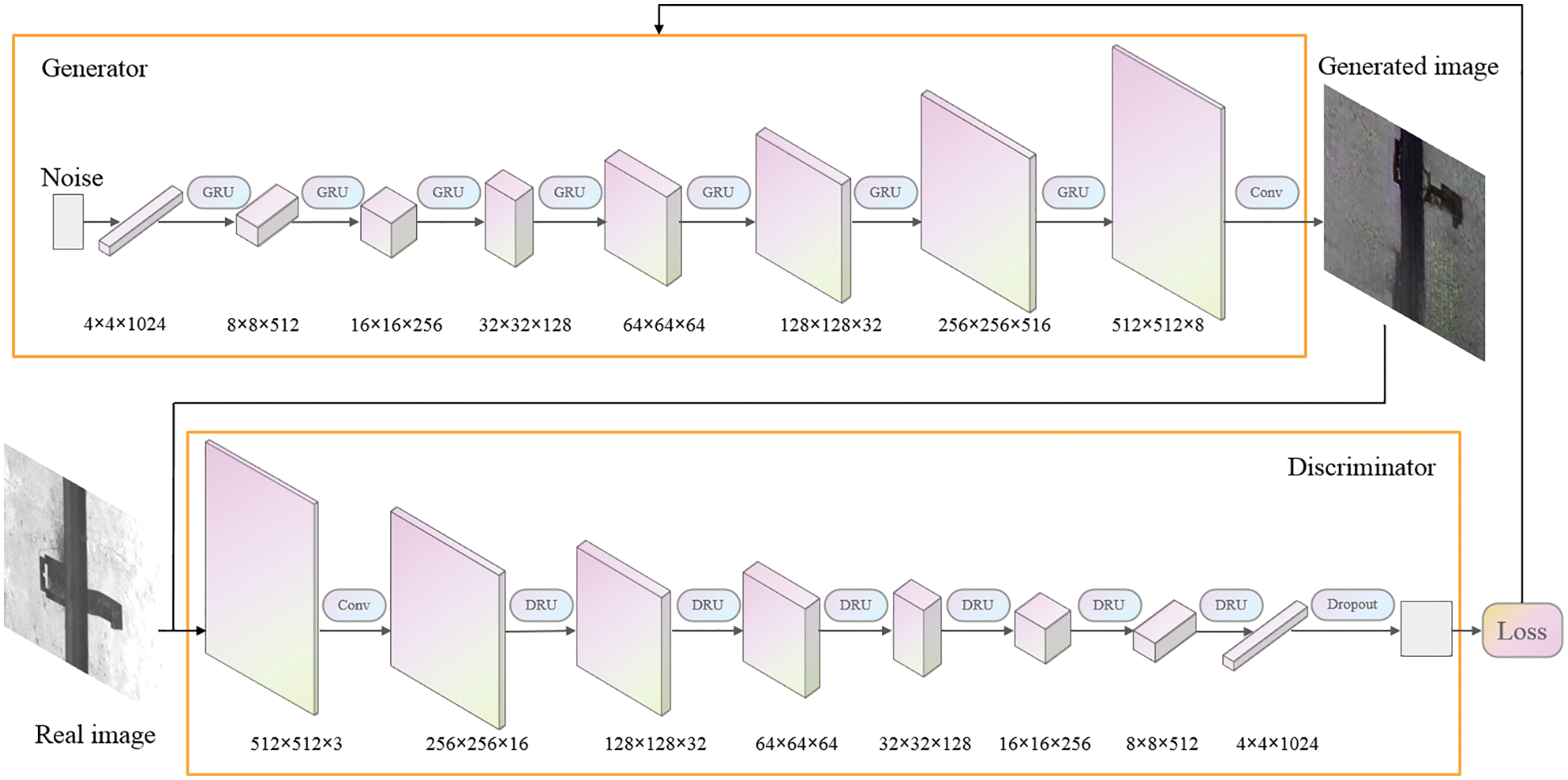
Figure 1: Structure of RW-DCGAN

Since the convolutional neural network needs backpropagation during the training process, if only the convolutional layer of the network is deepened, the number of model parameters will increase, which will cause gradient explosion or gradient disappearance in the model. To prevent such problems, we replace the deconvolution in the generator and discriminator with residual modules while deepening the network. Even if the network depth is deepened, the parameter quantity is greatly reduced compared to directly stacking convolutional layers, significantly improving the training speed. In addition, we also add the Dropout module, which can further filter out redundant parameters, prevent the model from overfitting, and enhance model generalization ability.

3.1.2 Generator and Discriminator

The improvements of the generator can be shown in Fig. 2. The improved residual module replaces the deconvolution in the original network with two convolution operations, which adopt the convolution kernel 3 × 3 and stride 1. Each residual unit implements the residual operation by increasing up-sampling. Moreover, the non-residual side uses the deconvolutional layer with kernel 1 × 1 and stride 2 for simple feature map upscaling to keep the same output size as the residual side. The improvements of the discriminator can be shown in Fig. 3. The improved residual module uses the convolutional layer with kernel 3 × 3 and stride 2, and the convolutional layer with kernel 3 × 3 and stride 1, respectively. To reduce the feature map, the non-residual side uses the deconvolution layer with kernel 1 × 1 and stride 2. Finally, the feature of the residual side and the non-residual side are superimposed as the output result.

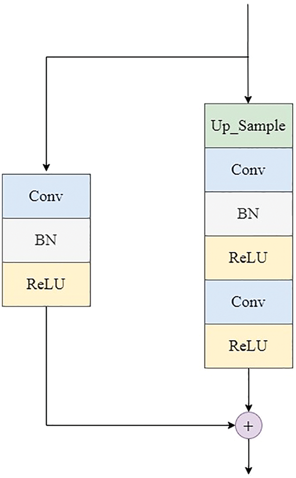
Figure 2: Residual module of generator

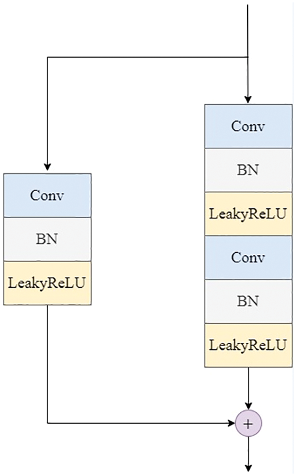
Figure 3: Residual module of discriminator

3.1.3 Loss Function

In order to improve the stability of the model, we use Wassertein distance instead of JS divergence [29,30], and the formula is expressed as follows:

W(Pdata,Pg)=infχ∼∏(Pdata,Pg)(E(x,y)∼χ[||x−y||])(1)

where Pg is the generated image distribution, Pdata is the real image distribution, and Π(Pdata, Pg) is the set of all possible joint distributions of combination Pg and Pdata. For each joint distribution χ, a real sample x and a generated sample y are obtained from the sampling, and the sample distance ||x−y|| and expectation of the distance are calculated. The lower bound of this expectation across all possible joint distributions is Wassertein distance. However, the lower bound cannot be solved directly, and the Lipschitz constant k needs to be introduced, so the formula can be expressed as follows:

k×W(Pdata,Pg)=maxa:||fa||LkEx∼Pdata[fa(x)]−Ex∼Pg[fa(x)](2)

All parameters of fa are limited to a certain range according to the actual situation, and the derivative of the input sample does not exceed a certain range at this time. So, there must be a constant k that satisfies the condition, and the loss functions of the generator and discriminator can be constructed. Their formulas are expressed as follows:

Lgenerator=−Ex−Pg[fα(G(x)](3)

Ldiscriminator=Ex∼Pg[fα(x)]−Ex∼Pdata [fα(x)](4)

3.2 GS-YOLOv5 Model

Deep learning can solve the problems of traditional methods that rely too heavily on datasets and physical methods that are time-consuming and labor-intensive. At the same time, the YOLOv5 model was chosen and modified accordingly to trade off the speed and accuracy of chuck detection. The speed of YOLOv5 is still insufficient to meet fixture detection needs, so it is still optimized for lightness.

3.2.1 Structure of GS-YOLOv5

The computational load of the network in deep learning mainly comes from the convolutional part, which has to be optimized in order to lighten the network. The algorithm based on deep learning can effectively obtain a large amount of feature information of the image, so we propose the GS-YOLOv5 model for leaky cable fixture detection, and the network structure is shown in Fig. 4.

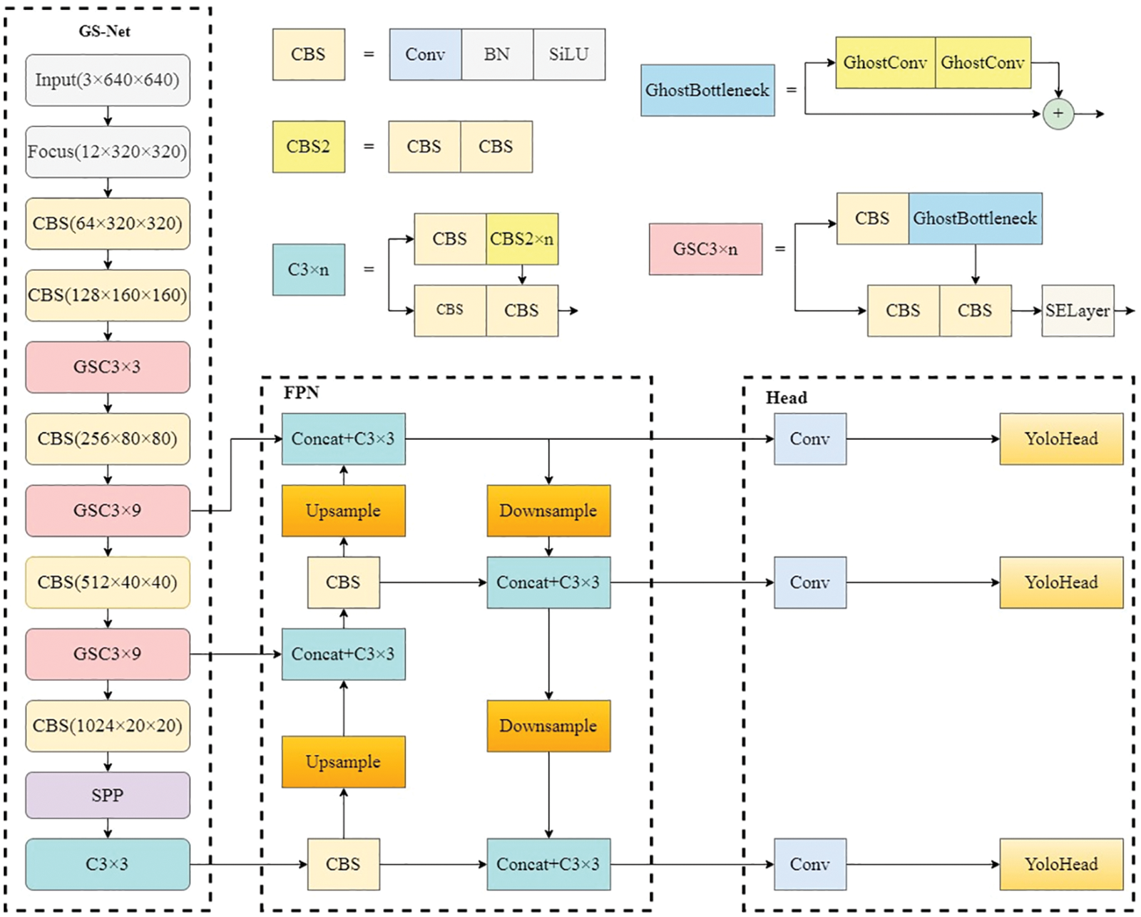
Figure 4: Structure of GS-YOLOv5

Since the backbone is a deep network, grouped convolution will inevitably cause information loss between channels. In addition, although Ghost convolution can reduce the extraction of redundant features [23], if a large number of Ghost convolutions are used, the feature extraction ability will also decrease. Therefore, we properly retain the standard convolution in the backbone of the network, and use Ghost convolution to replace the standard convolution only in the residual block. The attention mechanism is only inserted in the C3 module of residual blocks to enhance the feature extraction performance. The GS-YOLOv5 model was constructed by replacing the backbone network of YOLOv5 with the backbone network GS-Net, which incorporated the Ghost module and SENet. The size of the input image is smaller than possible, mainly due to the design of the feature fusion structure that is now adopted. Objects of different sizes are divided into different feature maps for processing, and the best size is between 400 × 400 and 800 × 800. And small objects perform better with larger input sizes, and the larger the input image, the greater the amount of computation, resulting in a decrease in detection speed [31]. The input image size of the model is 640 × 640 × 3. After passing the GS-Net backbone network consisting of several convolutional modules and GSC3, C3, and SPP modules, three different levels of feature maps are obtained. Next, these three different levels of feature maps are fused to obtain the detection results of the three different levels of feature maps, and finally, the results are presented.

3.2.2 Ghost Convolution

Although rich feature maps can be obtained through neural networks, if only standard convolutions are used to generate these feature maps, it may cause waste of computing resources and storage resources. Assume that the input feature map is X∈Rc×h×w, where c, h, w are the number of channels, height and width of the input feature map. And the output feature map is Y∈Rn×h′×w′, where n, h′, w′ are the number of channels, height and width of the output feature map. The formula of standard convolution can be expressed as follows:

Y=X∗f+b(5)

where b is the offset term, f∈Rc×k×k×n is the convolution filter, k is the kernel size, and the parameter quantity of standard convolution can be expressed as n⋅c⋅k⋅k. Ghost convolution is mainly composed of standard convolution and linear operation, which can reduce redundant feature information, learning cost of non-critical features, and computing resources required by the network [32]. Firstly, the input feature map X∈Rc×h×w is convolved with m standard convolutions of c⋅k⋅k, and obtain the original feature map Y′∈Rm×h′×w′, where m≤n and m=n/s. So, the parameter quantity of the original part in Ghost can be expressed as (n/s)⋅c⋅k⋅k. Then, perform s−1 linear operations on the original feature map, and superimpose the resulting s−1 feature maps and original feature map together to obtain the final output feature map Y∈Rn×h′×w′. The linear operation adopts (s−1)⋅(n/s) single-channel linear kernels with d⋅d, and the compression ratio can be written as follow:

rc=n⋅c⋅k⋅kns⋅c⋅k⋅k+(s−1)⋅ns⋅d⋅d≈s⋅cs+c−1≈s(6)

According to the above analysis, Ghost convolution can compress the parameter quantity to 1/s of the standard convolution. Therefore, using Ghost convolution can further improve the detection speed of the model.

3.3 Model Compression and Grad-CAM

3.3.1 Compression Strategy

The implementation process of channel pruning is simple, the compression efficiency is high, and the detection accuracy can be fine-tuned to find a suitable model, so we use channel pruning to achieve model compression [33]. Due to the large depth of the backbone, in order to prevent the model from overfitting and speed up the model convergence, we use the absolute value of the scaling factor γ of the BN layer to measure the importance of the channel. The normalization formula of the BN layer is expressed as:

Zout=γ×Zin−μσ2+ε+β(7)

where μ is the mean of the input feature map, σ2 is the variance, and β is the bias. If the value of γ is small, the corresponding output function Zout will be correspondingly smaller, and such channels can be clipped. During training, sparsity is achieved by adding a L1 regularity constraint of γ to the loss function. The formula is written as follows:

Lout=∑(x,y)l(f(x,W),y)+sr∑y∈Γg(γ)(8)

The first term is the training loss of the network. x and y are the input and output of the training, respectively, and W is the training parameter in the network. The second term is the regularity constraint, where g(γ)=|γ| and sr is the penalty coefficient to balance the two loss terms. After sparse training, the closer the channel pruning factor is to 0, the less important the channel is. Therefore, such channels also need to be pruned to obtain a more lightweight model. As the pruning rate increases, the model compression effect will get better and better, but the accuracy will also decrease. Fine-tuning can be used to fix the accuracy of the network so that the model can meet the needs of detection accuracy.

3.3.2 Crad-CAM Vision

To visualize the training process of the model, Grad-CAM uses the output for backpropagation to get the contribution of each pixel in the feature map [34]. The formula is expressed as follows:

αkc=1Z∑i∑j∂yc∂Aijk(9)

where αkc represents the contribution of the k-th feature map to category c, yc represents the prediction score of the network for category c, Z is the size of the feature map, and Aijk represents the pixel (i,j) of the k-th feature map. According to the degree of contribution, all feature maps are weighted and summed, and Grad-CAM is obtained through the ReLU activation function. The formula is defined as follows:

LGrad−CAMc=ReLU(∑kαkcAk)(10)

When the contribution value is less than 0, this part of the feature map has no positive effect on the classification result, so it is necessary to use the ReLU to remove the part less than 0. Grad-CAM can display the key areas of the input image and intuitively reflect the influence of each part of the original image on the detection result.

4  Experiments

This section will present a more detailed introduction to leaky cable fixture detection. To verify the excellent performance of our model proposed in this paper, we have performed extensive ablation studies and comparative experiments. We first conducted ablation experiments to verify the performance of the Ghost and SE modules. Besides, we performed sparse training and fine-tuned the model by cropping, then trained other mainstream models to compare with this paper’s model, and finally verified that our model was superior by visualization.

4.1 Experimental Environment and Evaluation Metrics

The whole experiment is conducted on the Windows10 operating system, the CPU is Intel(R) Core (TM) i7-8750H CPU@2.20GHZ, the GPU is NVIDIA GeForce GTX 1050Ti, the deep learning framework is based on Pytorch1.8 and CUDA10.2, the initial learning rate of the model is 0.001, and the momentum parameter is 0.937. In the learning rate update, the warmup method is used to adjust the learning rate so that the model converges faster and the effect is better. We use the mean average precision (mAP), parameter quantity, model volume, and FPS as the evaluation metrics.

4.2 Fixture Data and Data Augmentation

In this section, the fixture data will be introduced in detail. A high-speed camera needs to be placed on the window of trains. As shown in Fig. 5a, we choose a CMOS dual-line camera for the whole shooting process. Then we collect fixture images during the whole train journey. Since the camera has its light source and is always open for the entire working time, the lighting is stable throughout the shooting. The normal fixture is shown in Fig. 5b, and the faulty fixture is shown in Fig. 5c. Since the number of normal fixtures is vast, we only perform augmentation operations on the faulty fixtures.

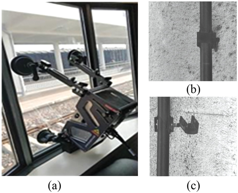
Figure 5: The camera and leaky cable fixture. (a) The CMOS dual-line camera. (b) The normal fixture. (c) The faulty fixture

In order to verify the superiority of the RW-DCGAN model proposed in this paper, we will conduct comparison experiments of the output fixture image, and the results are shown in Table 1. We show the augmentation effect of GAN, DCGAN, and RW-DCGAN on fixture images. It can be found that after multiple epochs of training, the quality of output images generated by GAN and DCGAN is not high, and the fixture part features are blurred and indistinguishable. Thanks to the inclusion of the W distance loss function and Dropout, for the same number of training session. The images generated by the proposed RW-DCGAN are clear and significantly outperform other models. Because of the residual network, the image quality of our proposed model is higher than others and closer to the real tunnel fixture picture. A total of 1500 faulty fixtures and 1500 normal fixtures are used in the experiment, which are divided into the training set, validation set and test set according to the ratio of 3:1:1.

4.3 Experiments Main Results

4.3.1 Ablation Experiment

In order to verify the effectiveness of our method, we designed ablation experiments by adding the proposed modules gradually. As shown in Table 2, after adding SENet, the model volume, parameter quantity, and detection speed decreased slightly, while mAP increased. It can prove that the attention mechanism can improve network recognition accuracy. If only Ghost is added, the model volume and parameter quantity are reduced, and the mAP is reduced by 0.8%. Although the precision is slightly lost, the detection speed is greatly improved compared to the YOLOv5 model. This is enough to show that Ghost convolution not only reduces the number of parameters, but also speeds up detection. After adding both SENet and Ghost, the model volume and parameters are significantly reduced, mAP is increased by 5.1% compared with YOLOv5, and the speed has no obvious change compared with G-YOLOv5, which also reflects that the improved model in this paper has more advantages.

4.3.2 Model Compression

We set different penalty coefficient s for sparse training of GS-YOLOv5. In the sparse training and clipping sections, the penalty coefficient is selected. Generally, the penalty factor needs to be higher, which will cause the model to be sparse too slowly. The sparseness effect is not good, and the penalty coefficient is too high to cause a significant loss of accuracy, so the penalty coefficient is generally set between 0.0001 and 0.005. The values of s in the experiment are 0.0001, 0.0005, 0.001, and 0.005, respectively. Fig. 6 shows the effect of different penalty coefficients on mAP during training.

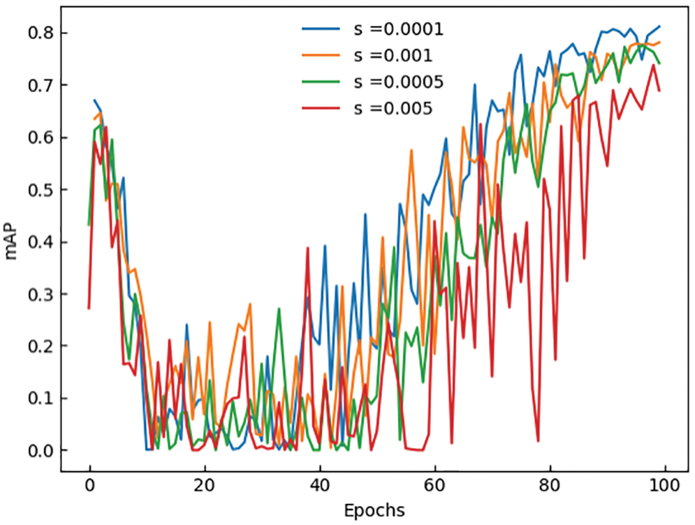
Figure 6: The line curve of mAP with different penalty coefficients

In order to express the sparsity effect more intuitively, we draw the γ distribution changes corresponding to different penalty coefficient s, as shown in Fig. 7. When s is 0.005, the γ distribution basically tends to 0. Due to the large loss of accuracy, it is difficult to recover in the later stage. When s is 0.0001, the γ distribution still mostly does not tend to 0. Although the accuracy is preserved, the improvement in model volume and speed is limited. To balance the detection accuracy and model volume, we set s to 0.0005 or 0.001.

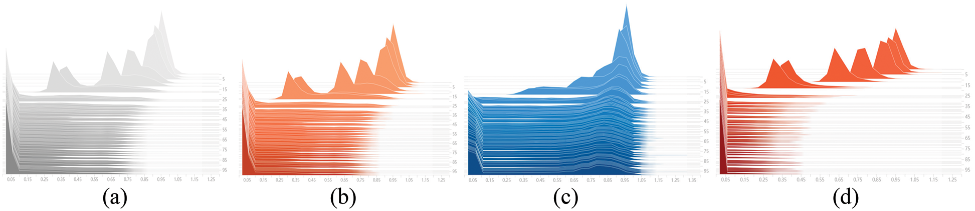
Figure 7: The line curve of γ distribution with different penalty coefficients. (a) s = 0.001 (b) s = 0.0005 (c) s = 0.0001 (d) s = 0.005

To obtain the best penalty coefficient s, we set the pruning ratio (pr) as 50%, 60%, 70%, 80%, and the detection results of pruning and fine-tuning can be shown in Table 3.

It can be found that when s is set to 0.0005, fine-tuning can play a great role, and the detection speed is significantly higher than that when s is 0.001. With the increase of the pruning ratio, although model volume and parameter quantity will be significantly reduced, and detection speed will increase, mAP will also decrease. After comprehensive comparison and analysis, we finally selected the GS-YOLOv5 with a pruning ratio of 70% and set s to 0.0005. In order to reflect the training process more intuitively, we show the mAP value with different coefficients and different pruning ratios in Fig. 8.

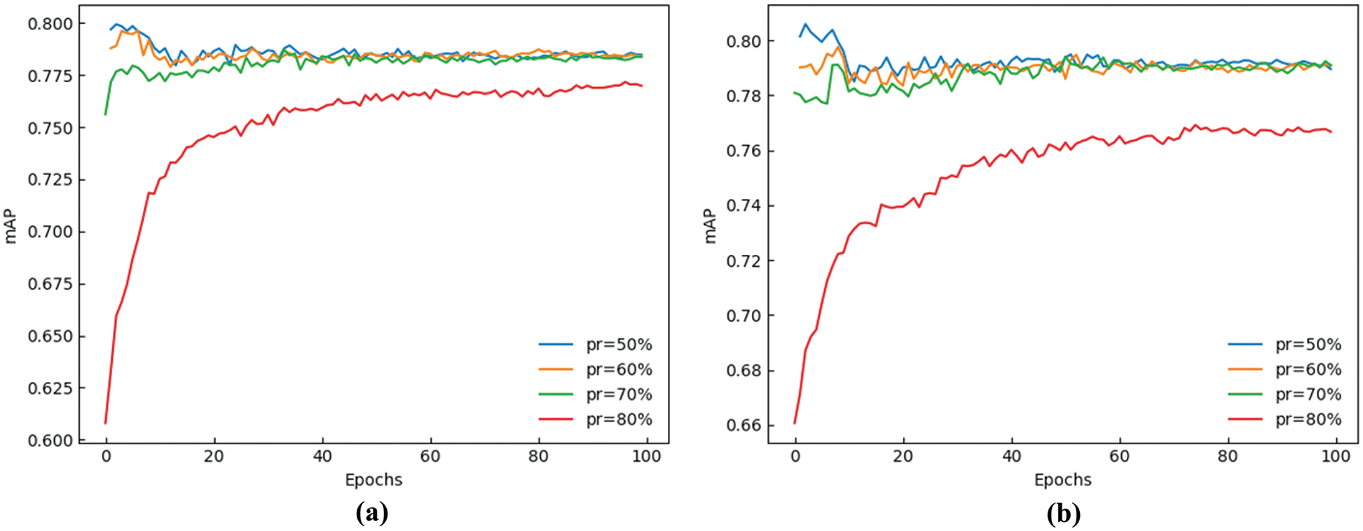
Figure 8: The line curve of mAP with different penalty coefficients and pruning ratios. (a) s = 0.001 (b) s = 0.0005

4.4 Comparison Analysis

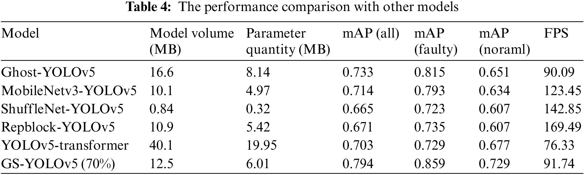
To sufficiently verify the excellent performance of our method, we compare the GS-YOLOv5 70% pruning with other mainstream models. As shown in Table 4, Ghost-YOLOv5 is to replace all standard convolutions in the backbone with Ghost convolution, and MobileNetv3-YOLOv5 is to replace the backbone with MobileNetv3 [35]. ShuffleNet-YOLOv5 is to replace the backbone with ShuffleNetv2 [36]. Repblock-YOLOv5 is to replace standard convolution with Repblock in the backbone. YOLOv5-transformer is to add the transformer module to the backbone. The results show that the lightweight networks MobileNetv3, ShuffleNet, and Repblock have faster speeds because their overall network layers are less, the number of parameters calculated is also less, but their mAP is low. Because of the low number of network layers, the extracted feature map needs to be improved, eventually decreasing the accuracy rate. Because the accuracy is too low, the detection of fixtures is prone to miss detection, misdetection, and other phenomena, which is challenging to meet the needs of fixture detection. Other networks are also inferior to GS-YOLOv5 (70%) in accuracy and speed. Therefore, this paper proposes that GS-YOLOv5 (70%) is more suitable for tunnel fixture detection.

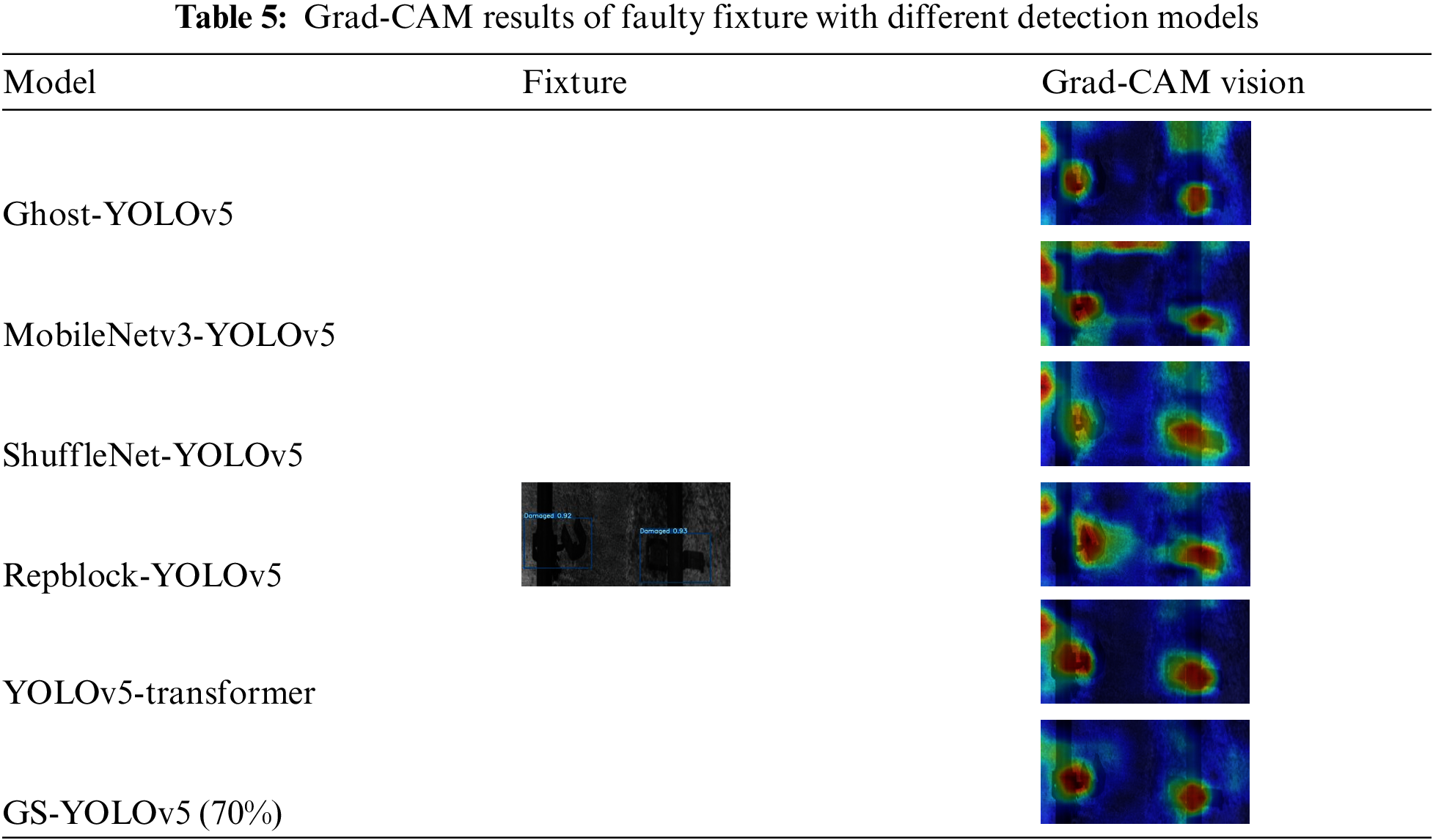
To visualize the areas of network attention, we obtain thermal maps for faulty fixtures with the Grad-CAM algorithm, and the comparison results are shown in Table 5. It can be found that these comparison models focus not only on the fixture areas, but also pay attention to other background areas in the tunnel. Because the model in this paper incorporates an attention mechanism that allows the model to focus more on the card tool, factors such as context have less influence on the model proposed in this paper. The model proposed in this paper has a high concentration, which can effectively reflect the fixture area and obtain fixture characteristics. This also highlights the superiority of the GS-YOLOv5 model.

5  Conclusion

This paper presents an effective method for detecting faulty fixtures. The method first proposes an RW-DCGAN to enhance the faulty fixture data, obtains higher-quality fixture images by adding a residual network, and uses a Wasserstein loss function to improve training stability. The Dropout module is also added to enhance the model’s generalization ability, solving the problems of single variation, unstable GAN training and poor quality of generated images in traditional methods. Secondly, GS-YOLOv5 is proposed to enhance fixture detection. Ghost convolution and SENet can filter the redundant information, which improves the detection accuracy by 5.1% and the detection speed by 3.5 fps. Finally, we used a model compression strategy to trim the redundant channels. The final model with a sparsity coefficient of 0.0005 and a trimming ratio of 70% gave the best results through experimental comparison. After fine-tuning the model, the speed was improved by11.32 fps with a 3% decrease in accuracy. The final model has a 2.1% increase in accuracy and 14.82 fps faster than YOLOv5. The number of parameters has been reduced by 70%, increasing detection speed without loss of accuracy. Next, we will conduct research related to diverse classification of damaged fixtures.

Funding Statement: This work was supported by the National Natural Science Foundation of China (No. 61702347, No. 62027801), Natural Science Foundation of Hebei Province (No. F2022210007, No. F2017210161), Science and Technology Project of Hebei Education Department (No. ZD2022100, No. QN2017132), Central Guidance on Local Science and Technology Development Fund (No. 226Z0501G), National innovation and Entrepreneurship training program for college students (No. 202110107024).

Availability of Data and Materials: The data used to support the findings of this study are available from the corresponding author upon request.

Conflicts of Interest: The authors declare that they have no conflicts of interest to report regarding the present study.

References

1. P. Liu, J. Feng, W. Ge, H. Wang, D. Wang et al., “A system-level performance evaluation for a 5g system under a leaky coaxial cable MIMO channel for high-speed trains in the railway tunnel,” Electronics, vol. 11, no. 8, pp. 1185–1197, 2022. [Google Scholar]

2. W. Liu, K. Quijano and M. M. Crawford, “YOLOv5-tassel: Detecting tassels in RGB UAV imagery with improved YOLOv5 based on transfer learning,” IEEE Journal of Selected Topics in Applied Earth Observations and Remote Sensing, vol. 15, pp. 8085–8094, 2022. https://doi.org/10.1109/JSTARS.2022.3206399 [Google Scholar] [CrossRef]

3. J. Wang, T. Xiao, Q. Gu and Q. Chen, “YOLOv5_CSL_F: YOLOv5’s loss improvement and attention mechanism application for remote sensing image object detection,” in 2021 Int. Conf. on Wireless Communications and Smart Grid, pp. 197–203, 2021. https://doi.org/10.1109/ICWCSG53609.2021.00045 [Google Scholar] [CrossRef]

4. A. Albayrak and M. S. Özerdem, “Gas cylinder detection using deep learning based YOLOv5 object detection method,” in 2022 7th Int. Conf. on Computer Science and Engineering, pp. 434–437, 2022. https://doi.org/10.1109/UBMK55850.2022.9919478 [Google Scholar] [CrossRef]

5. D. -H. Shin, D. -H. Jung, D. -C. Kim, J. -W. Ham and S. -O. Park, “A distributed FMCW radar system based on fiber-optic links for small drone detection,” IEEE Transactions on Instrumentation and Measurement, vol. 66, no. 2, pp. 340–347, 2017. https://doi.org/10.1109/TIM.2016.2626038 [Google Scholar] [CrossRef]

6. M. Niu, K. Song, L. Huang, Q. Wang, Y. Yan et al., “Unsupervised saliency detection of rail surface defects using stereoscopic images,” IEEE Transactions on Industrial Informatics, vol. 17, no. 10, pp. 6731–6741, 2021. [Google Scholar]

7. M. Zheng, Z. Lei and K. Zhang, “Intelligent detection of building cracks based on deep learning,” Image and Vision Computing, vol. 103, pp. 103987, 2020. [Google Scholar]

8. Y. Zhang, P. Yang and W. Li, “Detection of leakage cable fixture in tunnel based on feature enhancement SSD,” Journal of Beijing Jiaotong University, vol. 45, no. 2, pp. 105–110, 2021. [Google Scholar]

9. H. Ma, “Research and realization of tunnel leaky cable fixture fault detection system based on deep learning,” Master’s thesis, Institute of Information Science and Engineering, Hebei University of Science and Technology, Hebei, China, 2021. [Google Scholar]

10. Y. Zhang, Z. Song and W. Guo, “Multi-scale continuous gradient local binary pattern (mcg-lbp) for leaky cable fixture detection in high-speed railway tunnel,” IEEE Access, vol. 9, no. 11, pp. 147102–147113, 2021. [Google Scholar]

11. Y. Peng, “A vehicle detection system based on visual image of the cable fault,” Master’s thesis, School of Electronic and Information Engineering, Beijing Jiaotong University, Beijing, China, 2021. [Google Scholar]

12. J. Perng, Y. Hsu, Y. Yang, C. Chen and T. Ying, “Development of an embedded road boundary detection system based on deep learning,” Image and Vision Computing, vol. 100, pp. 103935, 2020. [Google Scholar]

13. Y. A. Yucesan and F. Viana, “Hybrid physics-informed neural networks for main bearing fatigue prognosis with visual grease inspection,” Computers in Industry, vol. 125, pp. 103386, 2021. [Google Scholar]

14. K. Jang, H. Jung and Y. An, “Automated bridge crack evaluation through deep super resolution network-based hybrid image matching,” Automation in Construction, vol. 137, pp. 104229, 2022. [Google Scholar]

15. J. Wu, Z. Zhao, C. Sun, R. Yan and X. Chen, “Few-shot transfer learning for intelligent fault diagnosis of machine,” Measurement, vol. 166, no. 15, pp. 108202, 2020. [Google Scholar]

16. H. Xu, Y. Huang and M. Liu, “Research of pest detection and identification of corn leaf based on improved YOLOv3 model,” Journal of Nanjing Agricultural University, vol. 122, no. 6, pp. 1–12, 2022. [Google Scholar]

17. S. Kim, “ECAP-YOLO: Efficient channel attention pyramid YOLO for small object detection in aerial image,” Remote Sensing, vol. 12, no. 23, pp. 4851, 2021. [Google Scholar]

18. Y. Cai, T. Luan, H. Gao, H. Wang, L. Chen et al., “YOLOv4-5D: An effective and efficient object detector for autonomous driving,” IEEE Transactions on Instrumentation and Measurement, vol. 70, pp. 4503613, 2021. [Google Scholar]

19. J. Li, W. Li, Y. Chen and J. Gu, “A PCB electronic components detection network design based on effective receptive field size and anchor size matching,” Computational Intelligence and Neuroscience, 2021, pp. 1–19, 2021. [Google Scholar]

20. A. G. Howard, M. Zhu, B. Chen, D. Kalenichenko, W. Wang et al., “Mobilenets: Efficient convolutional neural networks for mobile vision applications,” in IEEE Conf. on Computer Vision and Pattern Recognition, Honolulu, HI, USA, pp. 1–9, 2017. [Google Scholar]

21. Y. Zeng, L. Zhang, J. Zhao, J. Lan and B. Li, “JRL-YOLO: A novel jump-join repetitious learning structure for real-time dangerous object detection,” Computational Intelligence and Neuroscience, 2021, pp. 1–16, 2021. [Google Scholar]

22. X. Zhang, X. Zhou, M. Lin and J. Sun, “Shufflenet: An extremely efficient convolutional neural network for mobile devices[C],” in Proc. of Conf. on Computer Vision and Pattern Recognition, Salt Lake City, UT, USA, pp. 6848–6856, 2018. [Google Scholar]

23. K. Han, Y. Wang, Q. Tian, J. Guo, C. Xu et al., “Ghostnet: More features from cheap operations,” in Proc. of the IEEE/CVF Conf. on Computer Vision and Pattern Recognition, pp. 1580–1589, Seattle, WA, USA, 2020. [Google Scholar]

24. Y. Wang, “A mathematical introduction to generative adversarial nets (GAN),” arXiv:2009.00169, 2020. [Google Scholar]

25. A. Radford, L. Metz and S. Chintala, “Unsupervised representation learning with deep convolutional generative adversarial networks,” in Proc. of the Int. Conf. on Learning Representation, San Juan, Puerto Rico, pp. 1–16, 2016. [Google Scholar]

26. Y. Chen, Y. Wang, M. Kao and W. Chuang, “Deep photo enhancer: Unpaired learning for image enhancement from photographs with Gans,” in Proc. of the IEEE Conf. on Computer Vision and Pattern Recognition, Salt Lake City, UT, USA, pp. 6306–6314, 2018. [Google Scholar]

27. Z. Ni, W. Yang, S. Wang, L. Ma and S. Kwong, “Towards unsupervised deep image enhancement with generative adversarial network,” IEEE Transactions on Image Processing, vol. 29, pp. 9140–9151, 2020. [Google Scholar]

28. Y. Liu, Z. Wang, R. Geng, H. Zheng and Y. Zeng, “Structure preserving extremely low light image enhancement with fractional order differential mask guidance,” in Proc. of the 2nd ACM Int. Conf. on Multimedia, New York, NY, USA, pp. 1–7, 2021. [Google Scholar]

29. V. M. Panaretos and Y. Zemel, “Statistical aspects of wasserstein distances,” Annual Review of Statistics and Its Application, vol. 6, no. 1, pp. 405–431, 2019. [Google Scholar]

30. Y. Ding and X. M. Wang, “Naive Bayesian classification algorithm based on improved feature weighting,” Application Research of Computers, vol. 36, no. 12, pp. 3597–3600, 2019. [Google Scholar]

31. L. Qi, J. Kuen, J. Gu, Z. Lin, Y. Wang et al., “Multi-scale aligned distillation for low-resolution detection,” in 2021 IEEE/CVF Conf. on Computer Vision and Pattern Recognition, Nashville, TN, USA, pp. 14438–14448, 2021. https://doi.org/10.1109/CVPR46437.2021.01421 [Google Scholar] [CrossRef]

32. Y. Zhang, Z. Song and W. Li, “Enhancement multi-module network for few-shot leaky cable fixture detection in railway tunnel,” Signal Processing: Image Communication,vol. 113, pp. 116943, 2023. https://doi.org/10.1016/j.image.2023.116943 [Google Scholar] [CrossRef]

33. Z. Liu, J. Li, Z. Shen, G. Huang, S. Yan et al., “Learning efficient convolutional networks through network slimming,” in Proc. of the Int. Conf. on Computer Vision, Venice, Italy, pp. 2736–2744, 2017. [Google Scholar]

34. R. Ramprasaath, D. Abhishek, V. Ramakrishna, C. Michael, P. Devi et al., “Grad-CAM: Why did you say that? visual explanations from deep networks via gradient-based localization,” in Proc. of the Conf. on Computer Vision and Pattern Recognition, Honolulu, HI, USA, pp. 618–626, 2017. [Google Scholar]

35. A. Howard, M. Sandler, B. Chen, W. Wang, L. Chen et al., “Searching for mobilenetv3,” in Proc. of the Int. Conf. on Computer Vision, Thessaloniki, Greece, pp. 1314–1324, 2019. [Google Scholar]

36. N. Ma, X. Zhang, H. Zheng and J. Sun, “Shufflenetv2: Practical guidelines for efficient CNN architecture design,” in Proc. of the European Conf. on Computer Vision, Munich, Germany, pp. 122–138, 2018. [Google Scholar]