3-Qubit Circular Quantum Convolution Computation Using the Fourier Transform with Illustrative Examples

1  Introduction

The fast Fourier transform-based convolution is widely used in signal/image processing, data-driven learning, big data vitalization, and deep convolutional neural networks numerous applications [1–5]. Building an efficient quantum convolution algorithm for science and engineering needs is challenging. One solution here might be to use the convolution property, which states that the Fourier transform of a convolution of two signals is the pointwise product of their Fourier transforms under suitable conditions. In quantum computation, the r-qubit quantum Fourier transform (QFT) is defined as the 2r-point discrete Fourier transform (DFT) of amplitudes of the quantum superposition of the signal of length 2r. Different algorithms and circuits for the QFT have been developed [6–9]. The direct application of the quantum Fourier transform for calculation of the convolution faces many difficulties, which are associated with finding gates for the multiplication of the Fourier transforms [10,11]. It should be noted that exists the opinion that the quantum convolution is “physically impossible” [12].

In this paper, we propose a method of quantum convolution which is described in detail using examples with 3 qubits. Note here that the convolution of length 2r, or r-qubit convolution, can be sequentially divided by short convolutions [13]. Therefore, the availability of short convolution circuits makes it possible to implement convolution calculations using examples with signals of length 2r, r≥3. The case is considered, when the discrete Fourier transform of one of the signals is known and only the QFT of another signal is calculated. The considered method of convolution can be used for linear time-invariant systems with the known frequency characteristics. The Fourier transform method is very efficient in computing convolution on a classical computer; the convolution reduces to multiplication. But it is this multiplication operation that is the most difficult step in calculating the quantum convolution using the Fourier transform. To overcome this obstacle, we propose to use an additional qubit, perform the corresponding permutation, and prepare a quantum superposition of qubits for the inverse QFT. The examples of circuits for the low-pass and high-pass filters are also given.

2  Background

Quantum computing promises fast solutions to many problems in several areas, including quantum signal/image processing and quantum machine learning [14–16]. In recent decades, many papers have been published with the main goal of extending traditional signal and image processing tasks and operations within quantum computing [17,18]. It is well known that efficient quantum algorithms exist and perform significantly faster than classical computers [19]. The basic concept in the quantum computation is the qubit described by the superposition of states |q1⟩=a|0⟩+b|1⟩. This qubit may be in one of the basis states |0⟩ and |1⟩ with probability p0=|a|2 and p1=|b|2, respectively. Therefore, |a|2+|b|2=1. The quantum superposition |q2⟩=a|0⟩+b|1⟩+c|2⟩+d|3⟩ is for two qubits which may be in four basis states with probabilities p0=|a|2, p1=|b|2, p2=|c|2, and p3=|d|2. Thus, a single qubit is described by 2 classical bits, two qubits by 4 bits, and so on, k qubits hold the same amount of information as 2k bits.

All computation operations over qubits, or multiqubit superposition of states, are described by unitary matrices. This is a major hurdle in the construction of quantum circuits for many of the traditional operations that are widely used in signal and image processing. They include the convolution and gradient operators. In medical image processing, the method of quantum edge detection was described in [20]. Later, the model of image representation known as the novel enhanced quantum representation (NEQR) has proven to be very suitable for extracting edges with Sobel gradients [21]. We also mention the quantum algorithm for the Kirsch and Prewitt operator-based edge extractions [22,23]. The computation of linear and circular convolution in quantum computation is still the open problem. If the traditional fast method of convoluting two signals is based on the DFT and is reduced to the pointwise multiplication of these transforms, then such multiplication in quantum computing must be performed or at least approximated by unitary transforms. Thus, the circuits for the QFT exist, but cannot be directly applied to calculate the convolution. Our inability to work with the QFT in the traditional way should lead us to develop additional methods and circuits that could solve this difficult problem. We believe that sooner or later this problem will be solved for many cases of the convolution.

3  Quantum Convolution

In this section, we describe the quantum scheme for the convolution of a signal fn, n0:=(N−1), in a linear time-invariant system (LTI), when its frequency characteristic Hp, p=0:(N−1), is given. The length is a power of two, N=2r,r>1. The N-point DFT of the signal is

Fp=∑n=0N−1fnWnp,p=0:(N−1).(1)

Here, W is the exponential coefficient WN=exp⁡(−i2π/N). For simplicity of calculation and drawing, we consider the N=8 case. For the quantum superposition of the given signal fn,

|fˇ⟩=∑n=07fn|n⟩,(2)

The quantum Fourier transform is described by the following 3-qubit superposition:

|ψ3(fˇ)⟩=18∑p=07FP|p⟩.(3)

Here, |n⟩ and |p⟩ denote the standard basis states. We consider that the signal fn was normalized, i.e.,

∑n=07|fn|2=1.(4)

The quantum algorithms for the Fourier transform are known, and the circuit unit element for the 3-qubit QFT can be represented as shown in Fig. 1. Here, for the permutation PX, the graphical ‘sort’ symbol is used. The inverse 3-qubit QFT is described by a similar circuit, only two gates, the phase shifts must be changes as

S¯=[100−i]→S=[100i]and T¯=[100e−iπ/4]→T=[100eiπ/4].(5)

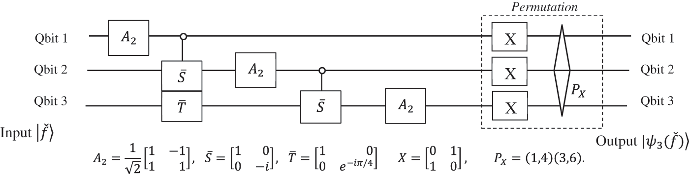
Figure 1: The quantum circuit for the 3-qubit QFT

We take the amplitudes of the transform in the order F7, F3, F5, F1, F6, F2, F4, and F0, as they are calculated in the above paired algorithm of the 3-qubit QFT [6]. After a permutation (1,5,3)(2,4), this transform can be written in the order F7, F1, F6, F2, F5, F3, F4, and F0. The corresponding 3-qubit superposition is

|ψ3(fˇ)⟩=18[(F7|0⟩+F1|1⟩)+(F6|2⟩+F2|3⟩)+(F5|4⟩+F3|5⟩)+(F4|6⟩+F0|7⟩)].(6)

The values of the frequency characteristic Hp of the system are considered in the same order. These two sequences of numbers should be multiplied pointwise, to obtain the Fourier transform of the convolution.

Yp=FpHp,p=7,1,6,2,5,3,4,0.(7)

Now, we consider the scheme given in Fig. 2. This scheme is for the state-wise multiplication of two qubits in matrix form,

|aˇ⟩=a0|0⟩+a1|1⟩   and   |bˇ⟩=b0|0⟩+b1|1⟩,(8)

by using the operation U. Here, a02+a12=b02+b12=1, or |a0|2+|a1|2=|b0|2+|b1|2=1, when the amplitudes are complex numbers.

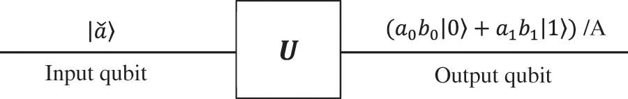
Figure 2: The abstract scheme for the operation U, (A=|a0b0|2+|a1b1|2)

After normalizing the superposition of qubits, this operation can be written in matrix form as

U|aˇ⟩=[b000b1][a0a1]=[b0a0b1a1]=a0b0|0⟩+a1b1|1⟩→1A(a0b0|0⟩+a1b1|1⟩),(9)

where the normalized coefficient for this new qubit is A=|a0b0|2+|a1b1|2. Thus, U=Ub1,b2 is the one-qubit operation. It can be considered as a Hermitian operator corresponding to the measurement of the qubit in the states of the computational basis. We consider the case when the numbers b0 and b1 are known and not equal to zero; there is no need to measure the qubit |bˇ⟩.

The diagonal matrix U can be considered with the determinant 1 as

U=Ub1,b2=1b0b1[b000b1]=1sin⁡(2φ)/2[cos⁡(φ)00sin⁡(φ)],(10)

for an angle φ∈[0,2π).

The following four matrices are defined:

U0=1H4H0[H400H0],U3=1H5H3[H500H3],U2=1H6H2[H600H2],

U1=1H7H1[H700H1].(11)

It is assumed that all numbers Hp≠0. The case when one of them is equal to zero should be considered separately. The scheme for multiplication of two transforms, Yp=FpHp, by using these four matrices, is shown in Fig. 3. The first two bits are used as control bits to apply one of these matrices. The matrix U0 is applied when the first two bits are 1. The matrix U3 is applied when the first two bits are 1 and 0, respectively. The matrix U2 is applied when these two bits are 0 and 1, and the matrix U1 is applied when the first two bits are 0.

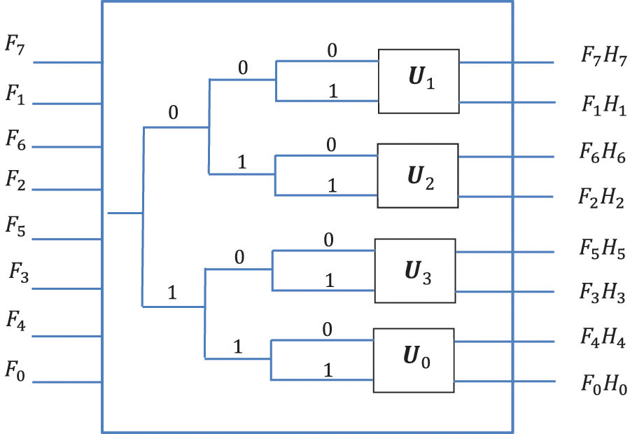
Figure 3: The scheme for the multiplication of transforms

In quantum computation, the matrices on one-qubit operators are unitary. Therefore, we consider the case when the signal fn is convoluted with a real impulse response hn of the filter or system. Then, there are three complex conjugate pairs, H7=H¯1, H6=H¯2, and H5=H¯3. Denoting by φ1, φ2, and φ3 the phases of the numbers H1,H2, and H3, respectively, we obtain the following three unitary matrices:

U3=[e−iφ300eiφ3],U2=[e−iφ200eiφ2],U1=[e−iφ100eiφ1].(12)

The numbers H4 and H0 are real, therefore the matrix U0 is considered to be the 2 × 2 identity matrix, I2. The matrices U1, U2, and U3 correspond to the Z-rotation gates of the amplitudes of qubits

Rz(ϑ)=[e−iϑ200eiϑ2],(13)

by the angles ϑ=2φ1, 2φ2, and 2φ3, respectively. Thus, Uk=Rz(2φk),k=0,1,2.

The scheme of multiplication of the transform Fp by the phase coefficients of the frequency characteristic Hp is shown in Fig. 4. Thus, this diagram is for the calculation of the transform FpHp/|Hp|.

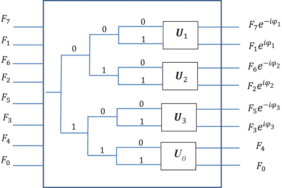
Figure 4: The scheme for the multiplication of the transform by phase coefficients

The same diagram as the quantum circuit is shown in Fig. 5. The first two qubits are the control qubits. A bullet in the line indicates that the control qubit is in state |1⟩, and an open circle indicates that the control qubit is in state |0⟩, when applying the operators Uk, k=0:3. One can see parallelism in computation that is the hallmark of quantum computing.

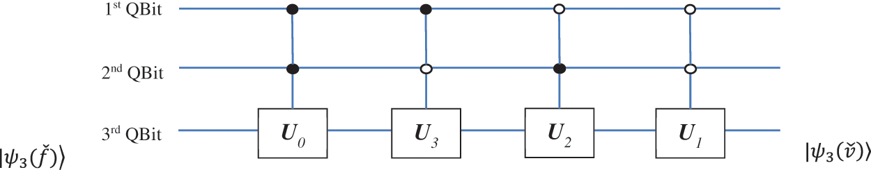
Figure 5: The quantum circuit for the multiplication of transform by the phase coefficients

The 3-qubit superposition that corresponds to the multiplication of the Fourier transform by the phase coefficients can be written as

|ψ3(vˇ)⟩=18[(F7e−iφ1|0⟩+F1eiφ1|1⟩)+(F6e−iφ2|2⟩+F2eiφ2|3⟩)+(F5e−iφ3|4⟩+F3eiφ3|5⟩)+ (F4|6⟩+F0|7⟩)].(14)

4  Multiplication of the Fourier Transforms

We consider an example of multiplication of 3-qubit Fourier transforms.

Example 1: If the impulse response is h=[1_1000000]/2, the discrete Fourier transform equals

H1=0.8536−0.3536i=0.9239e−i0.3927,   H7=H1¯,

H2=0.5−0.5i=0.7071e−i0.7854,     H6=H2¯,

H3=0.1464−0.3536i=0.3827e−i1.1781,    H5=H3¯,

H4=0,  H0=1.

The values of phases are φ1=−0.3927, φ2=−0.7854, and φ3=−1.1781.

To get the values Yp of the Fourier transform of the convolution yn, the amplitudes of the superposition |ψ3(vˇ)⟩ should be multiplied by magnitudes of the transfer function, as shown in Fig. 6.

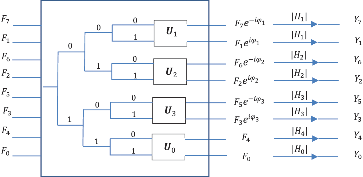
Figure 6: The abstract scheme for multiplication of the transforms

This operation is described by the diagonal matrix

D=diag{|H1|,|H1|,|H2|,|H2|,|H3|,|H3|,|H4|,|H0|}=(|H1|I2)⊕(|H2|I2)⊕(|H3|I2)⊕diag{|H4|,|H0|}(15)

For the above example, the diagonal matrix is

D=diag{0.9239,0.9239,0.7071,0.7071,0.3827,0.3827,0,1}.(16)

If the frequency characteristic has zeros, then we can consider adding a constant, Hp′=Hp+const. For instance, for the above example, we can take Hp′=Hp+1≠0, p=0:7. The impulse response function will be changed as hn′=hn+δn, i.e., the unit impulse will be added. The convolution changes as yn′=yn+fn. Therefore, the original convolution can be calculated as yn=yn′−fn, after measurement the convolution yn′.

The same control bits cannot be used for the multiplication by magnitudes |Hp| similar to how this was done for the scheme with the phase operators in Fig. 4. One-qubit operation

a|0⟩+b|1⟩→|H1|a|0⟩+|H1|b|1⟩(17)

is the identity transformation. It does not change the qubit, since the amplitudes of the basis states should be normalized. In other words, |H1|a|0⟩+|H1|b|1⟩=a|0⟩+b|1⟩, for any value of |H1|≠0. So we can think about rearranging the outputs to perform multiplication by the magnitudes |Hp| of the transfer function. For example, we consider the permutation P=(0,7)(2,6,4,5,3) that leads to the natural order of outputs, which is shown in Fig. 7.

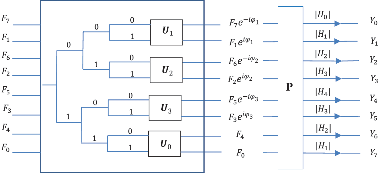
Figure 7: The abstract scheme for multiplication of the transforms with the permutation (P)

|ψ3(vˇ)⟩=18[F0|0⟩+F1eiφ1|1⟩+F2eiφ2|2⟩+F3eiφ3|3⟩+F4|4⟩+F5e−iφ3|5⟩ +F6e−iφ2|6⟩+F7e−iφ1|7⟩].(18)

We denote the amplitudes of this superposition by Vp and write

|ψ3(vˇ)⟩=18∑p=07Vp|p⟩.(19)

We denote by D the operator with this diagonal matrix and add it to the circuit as shown in Fig. 8.

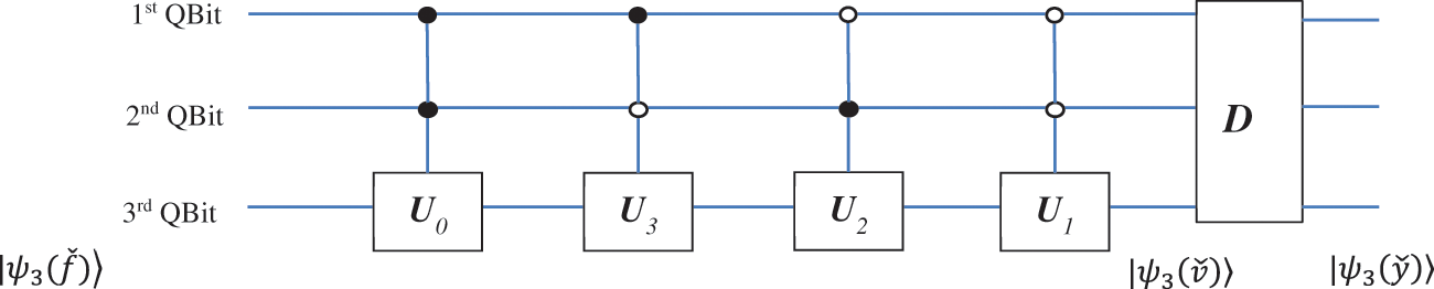
Figure 8: The abstract quantum circuit for the multiplication of the Fourier transforms

This operator can be viewed as the process of preparing the next quantum superposition from |ψ3(vˇ)⟩,

|ψ3(yˇ)⟩=1A[|H0|V0|0⟩+|H1|V1|1⟩+|H2|V2|2⟩+|H2|V3|3⟩+|H4|V5|4⟩+|H3|V5|5⟩+|H2|V6|6⟩+|H1|V7|7⟩].(20)

The normalized coefficient is

A=∑p=07|Yp|2=8∑n=07|yn|2.(21)

Thus, D is an operator of transition from one 3-qubit superposition to another. The amplitudes Vp, p=0:7, are calculated by the quantum scheme in Figs. 4 and 5, and the magnitudes of the transfer function |Hp| are given. For the convolution in Example 1, the quantum superposition for the convolution in frequency domain is

|ψ3(yˇ)⟩=1A[V0|0⟩+0.9239(V1|1⟩+V7|7⟩)+0.7071(V2|2⟩+V6|6⟩)+ 0.3827(V3|3⟩+V5|5⟩)].(22)

In quantum computing, this step relates to measurement. In other words, the operator D is the Hermitian operator specifying the measurement in a 3-qubit system in the computational basis,

D=|H0||0⟩⟨0|+|H1||1⟩⟨1|+|H2||2⟩⟨2|+|H3||3⟩⟨3|+|H4||4⟩⟨4|+|H3||5⟩⟨5|+|H6||6⟩⟨6|+|H1||7⟩⟨7|.(23)

The superposition |ψ3(yˇ)⟩ will be the input for the inverse 3-qubit QFT.

The above circuit of multiplication of the transforms with the measurements in Fig. 8 will be considered as a circuit element shown in Fig. 9.

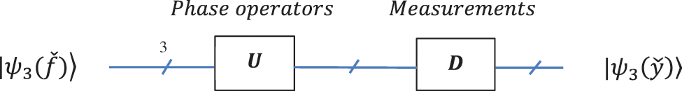
Figure 9: The abstract circuit element for the 3-qubit multiplication of the Fourier transforms

The complete quantum scheme for calculating the 3-qubit convolution is shown in Fig. 10.

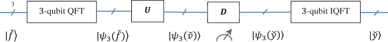
Figure 10: The scheme for computing the 3-qubit convolution of the signal

5  Ideal Low-Pass Filter in Example

It should be noted that the operation D can be placed before the phase operators, as shown in Fig. 11. Then, the superpositions

|ψ3(vˇ)⟩=1A∑p=07Vp|p⟩=1A∑p=07Fp|Hp||p⟩(24)

and

|ψ3(yˇ)⟩=1A[V0|0⟩+V1eiφ1|1⟩+V2eiφ2|2⟩+V3eiφ3|3⟩+V4|4⟩+V5e−iφ3|5⟩+ V6e−iφ2|6⟩+V7e−iφ1|7⟩].(25)

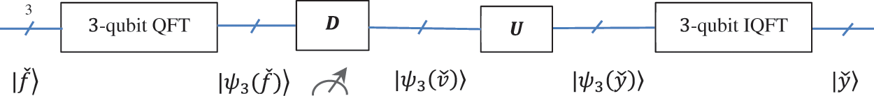
Figure 11: The scheme for computing the 3-qubit convolution of the signal

It is important to note that the operator D is not unitary. It could be added to the set of unitary operators of quantum computing to use the D operator in quantum circuits. The example below shows that it is possible to implement this operator without measurement and therefore solve the problem of quantum convolution at least for simple filters. Such filters are the low-pass, high-pass, and band-pass ideal filters.

Example 2: Consider the following ideal low-pass filter

Hp={1,p=0,eiπ/12,p=1,e−iπ/12,p=7,0,p=2,3,4,5,6.(26)

The impulse response h=(2.9319,2,0.4824,−0.7321,−0.9319,0,1.5176,2.7321)/8 of this filter is shown in Fig. 12.

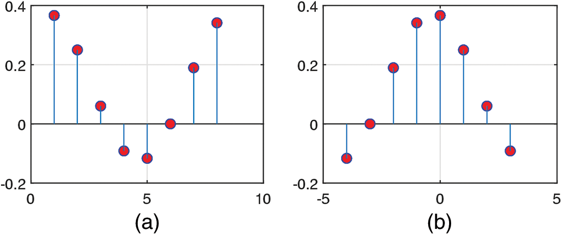
Figure 12: (a) The impulse response and (b) periodically shifted to the center

The discrete Fourier transform of the convolution yn=fn∗hn consists of only three components of the transform Fp, as shown in Fig. 13. The quantum Fourier transform of the convolution can be written as the following 3-qubit superposition:

|ψ3(yˇ)⟩=1A(Y0|000⟩+Y1|001⟩+Y7|111⟩)=1A(H0F0|000⟩+H1F1|001⟩+H7F7|111⟩).(27)

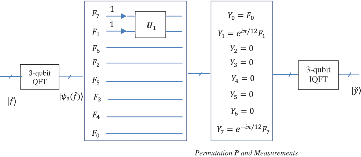
Figure 13: The scheme of calculation of the 8-point circular convolution

Thus, the input of the inverse 3-qubit QFT is the 3-qubit superposition

|ψ3(yˇ)⟩=1A(F0|000⟩+eiπ/12F1|001⟩+e−iπ/12F7|111⟩)(28)

with the normalized coefficient A=|F0|2+|F1|2+|F7|2. Here, U1 is the matrix of Z-rotation by the angle π/6,

U1=[e−iπ/1200eiπ/12],(29)

and the permutation P=(0,7)(2,6,4,5,3).

The only difficulty is understanding how to implement the quantum gates for the superposition in Eq. (28) after computing the 3-qubit QFT of the signal fn. Five amplitudes of the 3-qubit superposition are zeroed. To prepare this superposition |ψ3(yˇ)⟩, three qubits must be measured in the basis states |000⟩, |001⟩, and |111⟩. Since |H0|=|H1|=|H7|=1, the operator D can be considered the Hermitian operator specifying the measurement in a 3-qubit system in the computational basis

D=|0⟩⟨0|+|1⟩⟨1|+|H1||7⟩⟨7|=|000⟩⟨000|+|001⟩⟨001|+|111⟩⟨111|(30)

with the matrix representation D=diag{1,1,0,0,0,0,0,1}.

Let us see how the diagonal operator D can be included in a non-abstract quantum scheme using this example. We add one qubit, qubit number 4, as the zero qubit. In other words, we consider the 4-qubit register, wherein the second part is filled by zeros. This superposition is

|ψ4(yˇ)⟩=(F0,eiπ12F1,F6,F2,F5,F3,F4,e−iπ12F7)T⊕(0,0,0,0,0,0,0,0)T.(31)

Now, we consider a permutation that removes unnecessary information from the first part of the register for further processing. For instance, the permutation P4=(2,14,9,3,10,4,13,8)(5,11)(6,12) can be used,

P4:[F0eiπ12F1F6F2F5F3F4e−iπ12F7]⊕[00000000]→|ψ4(p)⟩=[F0eiπ12F100000e−iπ12F7]⊕[00F2F3F4F5F60].(32)

There are many permutations that result in the 16-dimensional vector with the first part equal (F0,e−iπ/12F1,0,0,0,0,0,e−iπ/12F7). It is also known, that if an operator is unitary, it can be implemented in a quantum computer [24,25]. Thus, we consider that P4 is a permutation that has a quantum circuit.

One more step is required to perform the 3-qubit quantum Fourier transform on the first part of the 4-qubit register/superposition. For that, the first qubit can be used as the control qubit. The 3-qubit QFT is performed when the first qubit is in the state 0. As a result, we obtain the circuit with the 4-qubit input, to calculate the 3-qubit convolution. This simplified circuit is shown in Fig. 14. The 3-qubit direct QFT and inverse QFT (IQFT) work in this circuit when the first qubit is in the state |0⟩.

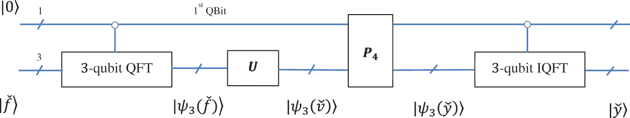
Figure 14: The quantum circuit for computing the 3-qubit convolution of the signal

If use the 3-qubit inverse QFT (IQFT) when the first qubit is in the state |1⟩, the result will be convolution of the signal with the high-pass filter

Hp={0,p=0,1,7,1,p=2,3,4,5,6.(33)

We can simplify the circuit for this high-pass filter, as shown in Fig. 15. There is no need to use the phase operator U, and the new permutation, P4=(0,8)(1,9)(2,6,4,5,3)(7,15), can be defined as

P4:|0⟩⊗∑p=07Fp|p⟩=[F0F1F6F2F5F3F4F7]⊕[00000000]→|ψ4(p)⟩=[00F2F3F4F5F60]⊕[F0F100000F7].(34)

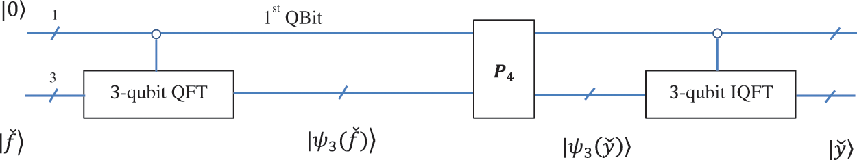
Figure 15: The circuit for computing the 3-qubit convolution of the signal for the high-pass filter

6  General Case of Convolution with Ideal Filters

We assume that such examples of filtering or quantum convolution over r qubits in the general case r > 3 can also be found. We can also go the other way when calculating the quantum convolution. The discrete paired transform allows to reduce the 2r-point cyclic convolution to the convolutions of lengths 2r−1,2r−2,…,8,4,2, and 1 [13]. This process can be continued until we get all cyclic convolutions of the order less than or equal to 8. The short convolutions, namely the 2-point and 4-point cyclic convolutions, or 1-and 2-qubit convolutions, have simple schemes of calculation. Indeed, the 1-qubit convolution is described by the unitary matrix

U=1h02+h12[h0h1h1h0].(35)

The 2-qubit convolution scheme can be described by the operations similar to the r=3 case above. For instance, for the real impulse response, the multiplication of the Fourier transform {F3,F1,F2,F0} by the phase coefficients and diagonal matrix D=diag{|H0|,|H1|,|H2|,|H1|} can be performed by the scheme shown in Fig. 16. This matrix represents the Hermitian operator of measurements in the 2-qubit system,

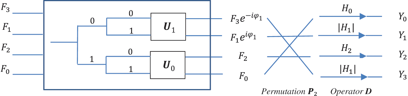
Figure 16: The scheme for multiplication of the 2-qubit transforms with the permutation

D=|H0||00⟩⟨00|+|H1||01⟩⟨01|+|H2||10⟩⟨10|+|H1||11⟩⟨11|.(36)

In this circuit, the permutation is P2=(0,3), i.e., P2:(0,1,2,3)→(3,1,2,0), and its matrix is

P2=[0001010000101000] and P2=(P2)−1.(37)

7  Conclusion

Implementing the circular convolution in quantum computers is difficult, but examples of convolution can be found. In this work, the convolution of a 3-qubit signal with another one is considered. The second signal is the impulse response of a linear time-invariant system, whose discrete Fourier transform is known or given. The abstract quantum scheme for the 3-qubit circular convolution is proposed. The examples with the low-pass and high-pass filters are described. The most interesting case is when the impulse response of the system is real. The only difficulty in implementing this algorithm in the general case is the implementation of D operation on qubits, i.e., the amplification of the amplitudes of the 3-qubit superposition based on the absolute values of the frequency characteristic of the system. To do this, we propose to use one additional qubit. Measurements of qubits can be used for this operation.

Acknowledgement: None.

Funding Statement: The authors received no specific funding for this study.

Author Contributions: The authors confirm contribution to the paper as follows: study conception and design: A. Grigoryan; methodology and data collection: A. Grigoryan; analysis and interpretation of results: A. Grigoryan, S. Agaian; draft manuscript preparation and structuring: A. Grigoryan, S. Agaian. All authors reviewed the results and approved the final version of the manuscript.

Availability of Data and Materials: All data generated or analyzed during this study are included in this published article.

Conflicts of Interest: The authors declare that they have no conflicts of interest to report regarding the present study.

References

1. K. Beer et al., “Training deep quantum neural networks,” Nat. Commun., 2020. doi: https://doi.org/10.1038/s41467-020-14454-2. [Google Scholar] [PubMed] [CrossRef]

2. S. Sahoo, A. K. Mandal1, P. K. Samanta, I. Basu, and P. Roy, “A critical overview on quantum computing,” J. Quantum. Comput., vol. 2, no. 4, pp. 181–192, 2020. [Google Scholar]

3. Y. Li, R. Zhou, Q. Xu, and J. Luo, “A quantum deep convolutional neural network for image recognition,” Quantum Sci. Technol., vol. 5, no. 4, 2020. doi: https://doi.org/10.1088/2058-9565/ab9f93. [Google Scholar] [CrossRef]

4. M. Altaisky, N. Kaputkina, and V. Krylov, “Quantum neural networks: Current status and prospects for development,” Phys. Part. Nuclei., vol. 45, pp. 1013–1032, 2014. [Google Scholar]

5. A. M. Grigoryan and S. S. Agaian, “Quaternion quantum image representation: New models,” in Proc. SPIE 11399, Mobile Multimedia/Image Processing, Security, and Applications 2020, 2020, vol. 11399, pp. 6. [Google Scholar]

6. A. M. Grigoryan and S. S. Agaian, “Paired quantum Fourier transform with log2N Hadamard gates,” Quantum Inf. Process., vol. 18, no. 217, pp. 26, 2019. [Google Scholar]

7. H. S. Li, P. Fan, H. Xia, S. Song, and X. He, “The quantum Fourier transform based on quantum vision representation,” Quantum Inf. Process., vol. 17, no. 333, pp. 25, 2018. [Google Scholar]

8. R. Cleve and J. Watrous, “Fast parallel circuits for the quantum Fourier transform,” in Proc. IEEE 41st Annual Symp. on Found. of Comput., Redondo Beach, CA, USA, 2000, pp. 526–536. [Google Scholar]

9. L. R. Perez and J. C. Garcia-Escartin, “Quantum arithmetic with the quantum Fourier transform,” Quantum Inf. Process, vol. 16, pp. 14, 2017. [Google Scholar]

10. A. M. Grigoryan and S. S. Agaian, “1-D convolution circuits in quantum computation,” Int. J. Sci. Eng. Res., vol. 11, no. 8, pp. 5, 2020. [Google Scholar]

11. S. Caraiman and V. I. Manta, “Quantum image filtering in the frequency domain,” Adv. Electr. Comp. Eng., vol. 13, no. 3, pp. 77–84, 2013. [Google Scholar]

12. C. Lomont, “Quantum convolution and quantum correlation are physically impossible,” arXiv: quant-ph/:0309070, 2003. [Google Scholar]

13. A. M. Grigoryan, “Resolution map in quantum computing: Signal representation by periodic patterns,” Quantum Inf. Process, vol. 19, no. 177, pp. 21, 2020. [Google Scholar]

14. S. K. Jeswal1 and S. Chakraverty, “Recent developments and applications in quantum neural network: A review,” Arch. Comput. Methods Eng., vol. 26, no. 3, pp. 15, 2018. [Google Scholar]

15. M. Schuld, I. Sinayskiy, and F. Petruccione, “An introduction to quantum machine learning,” Contemp. Phys., vol. 56, no. 2, pp. 172–185, 2015. [Google Scholar]

16. J. Biamonte et al., “Quantum machine learning,” Nature, vol. 549, no. 7671, pp. 195–202, 2017. doi: https://doi.org/10.1038/nature23474. [Google Scholar] [PubMed] [CrossRef]

17. A. M. Grigoryan and S. S. Agaian, “New look on quantum representation of images: Fourier transform representation,” Quantum Inf. Process, vol. 19, no. 148, pp. 26, 2020. [Google Scholar]

18. F. Yan, A. M. Iliyasu, and S. E. Venegas-Andraca, “A survey of quantum image representations,” Quantum Inf Process, vol. 12, no. 1, pp. 1–35, 2015. [Google Scholar]

19. M. A. Nielsen and I. L. Chuang, “Introduction and overview,” in Quantum Computation and Quantum Information, 10th ed. New York, USA: Cambridge University Press, 2010, pp. 36–42. [Google Scholar]

20. X. Fu, M. Ding, Y. Sun, and S. Chen, “A new quantum edge detection algorithm for medical images,” in Proc. SPIE 7497, MIPPR 2009: Medical Imaging, Parallel Processing of Images, and Optimization Techniques, 2009, vol. 7497, pp. 7. [Google Scholar]

21. R. Chetia, S. M. B. Boruah, and P. P. Sahu, “Quantum image edge detection using improved Sobel mask based on NEQR,” Quantum Inf. Process, vol. 20, no. 21, 2021. [Google Scholar]

22. P. Xu, Z. He, T. Qiu, and H. Ma, “Quantum image processing algorithm using edge extraction based on Kirsch operator,” Opt. Express, vol. 28, no. 9, pp. 12508–12517, 2020. [Google Scholar] [PubMed]

23. R. G. Zhou, H. Yu, Y. Cheng, and F. X. Li, “Quantum image edge extraction based on improved Prewitt operator,” Quantum Inf. Process, vol. 18, no. 9, pp. 261, 2019. [Google Scholar]

24. A. Barenco and, “Elementary gates for quantum computation,” arXiv:quant-ph/9503016v1, 1995. [Google Scholar]

25. J. Kim, J. S. Lee, and S. Lee, “A general method to implement an arbitrary unitary operator in quantum computation,” arXiv:quant-ph/9908052, 2000. [Google Scholar]