Numerical Simulation of Residual Strength for Corroded Pipelines

1  Introduction

The integrity of energy transportation infrastructure has emerged as a critical global concern, particularly in pipeline systems that convey approximately 70% of the world’s oil and 99% of natural gas through steel conduits [1]. China has established an extensive oil and gas pipeline network, creating a comprehensive system that spans the nation and connects to international sources. However, as these pipeline systems age, they become increasingly susceptible to structural deterioration, with corrosion emerging as a predominant threat to operational safety. The severity of this issue is underscored by statistical evidence: between 2007 and 2017, China’s oil and gas network suffered more than 370 pipeline leakage incidents, resulting in 75 fatalities, economic losses surpassing 10 billion yuan, and 10 major environmental contamination events [2]. Recognizing these challenges, China’s 14th Five-Year Plan explicitly emphasizes the imperative of enhancing oil and gas pipeline safety to safeguard national economic security. For in-service pipelines, the assessment of remaining strength—which characterizes the maximum load-bearing capacity of defect-containing structures—serves as a crucial indicator for estimating remaining service life [3].

The evaluation of residual strength in corroded pipelines has evolved significantly through various methodological approaches. Contemporary assessment methods can be categorized into three distinct frameworks: standard-based methods, finite element analysis, and intelligent prediction methods [4]. Significant advances in finite element analysis have enabled increasingly sophisticated evaluations. Benjamin et al. [5] pioneered comprehensive experiments on buried pipelines with multiple corrosion points, developing an evaluation methodology based on finite element analysis. Building upon this foundation, Chen et al. [6] employed nonlinear finite element analysis to investigate failure pressure in high-strength pipelines with various corrosion configurations, establishing predictive regression equations. Further advancing the field, Cai et al. [7] introduced an innovative numerical simulation model that conceptualizes dents and metal loss as notches, enabling residual strength prediction based on bending moment and critical curvature parameters. Chin et al. [8] conducted a failure analysis of a corroded high-strength pipeline subjected to hydrogen damage using a finite element method (FEM) and a back-propagation neural network optimised by a genetic algorithm (GA-BP neural network), and developed a new bursting model that takes hydrogen damage into account. Zhang et al. [9] developed a finite element model to predict the residual strength of X80 steel pipe lines containing group corrosion defects. Zhou et al. [10] analysed the effect of uniform pitting corrosion on the residual ultimate strength of submarine pipelines using a nonlinear finite element method and proposed a mathematical formula to predict the residual ultimate strength of pipelines.

Recent developments in artificial intelligence have introduced promising alternatives for residual strength prediction. Feng et al. [11] demonstrated the efficacy of artificial neural networks in predicting failure pressure using a dataset of 71 pipeline burst tests. Subsequently, Lu et al. [12] advanced the field by developing an ensemble model incorporating relevance vector machine and multi-objective salp swarm algorithms, achieving notable success with existing burst pressure databases. Sun et al. [13] investigated the prediction of residual strength and life of elbow pipes with erosion defects by combining numerical simulation techniques and Genetic Algorithm Optimised Extreme Learning Machine (GA-ELM) approach. Wang et al. [14] used a dataset of 453 instances to predict the residual strength of corroded pipes by applying a stacked integrated learning model containing seven base learners and three meta learners. Lu et al. [15] proposed a new data-driven framework for predicting the residual strength of corroded pipelines. The dimensionality of the available data was reduced by Principal Component Analysis (PCA) to determine the input-output structure of the prediction model, and then Support Vector Machines (SVMs) based on Multi-Objective Optimisation (MOO) were used to predict the residual strengths of the pipelines, and the accuracy and stability of the model were taken into account in the MOO. Chen et al. [16] investigated the use of a multilayer perceptron (MLP) and a modified feedforward neural network (FFNN) to predict the residual strength of corroded pipes. The ReLU activation function and dropout method were used to reduce the number of neurons during ANN training, which improved the prediction accuracy of the model. Jiang et al. [17] developed an integrated deep learning-based model for assessing the residual strength of pipelines affected by random corrosion defects under internal pressure. The model combines random field theory, finite element analysis and convolutional neural networks to improve the accuracy and computational efficiency of managing the structural integrity of pipelines. Miao et al. [18] proposed a new method based on the HTLBO-DELM model for predicting the residual strength of pipelines. They used the Hybrid Teaching Optimisation Algorithm (HTLBO) to improve the prediction accuracy of the Deep Extreme Learning Machine (DELM) model, and trained and validated the model using experimental data. Li et al. [19] estimated the residual strength of the pipe by building a finite element model, then applied the Local Linear Embedding (LLE) algorithm to process the data and finally developed an intelligent model using the Bayesian Regularised Artificial Neural Network (BRANN) algorithm for prediction. Nevertheless, these intelligent methods remain constrained by their reliance on limited historical databases, lacking the capability for direct prediction from real-time inspection and monitoring data.

While these studies have significantly advanced our understanding of pipeline residual strength assessment, several critical gaps remain. First, most existing research focuses on theoretical modeling or experimental validation independently, whereas this study integrates both approaches through a comprehensive 1:12.7 scaled model validation framework. Second, while previous studies typically examine individual defect parameters, our research systematically investigates the interactive effects among defect dimensions, wall thickness, and failure patterns through a novel three-tier parameter grouping approach (random, deviation, and structural groups). Third, unlike existing studies that often rely on simplified defect geometries, our research incorporates actual inspection data from the Yichang-Qianjiang pipeline section to generate statistically representative defect distributions, enhancing the practical applicability of our findings. Furthermore, recent studies by Chun et al. [20] and Nam et al. [21] have demonstrated the importance of analyzing corroded steel surfaces and location-dependent capacity variations, respectively. Building upon their work, our study extends the analysis to incorporate multiple defect morphologies and their evolution patterns during the failure process [22,23], providing a more comprehensive understanding of pipeline failure mechanisms.

Within this context, the Yichang-Qianjiang section of the Sichuan-East Gas Pipeline represents a critical case study in pipeline integrity management. This vital infrastructure component, spanning 153.09 km with a 1016 mm diameter, has been operational since January 2009. Constructed with X70 grade steel and featuring variable wall thicknesses (17.5, 21.0, and 26.2 mm), the pipeline is designed to withstand a maximum operating pressure of 10 MPa. Following its initial internal inspection in 2015 and subsequent comprehensive internal and external inspections in 2023, the discovery of 389 corrosion defects has heightened the urgency for thorough strength assessment [24].

To address these complex challenges, this study establishes four primary objectives: (1) development of a comprehensive finite element model using ABAQUS for evaluating corroded pipeline residual strength, incorporating appropriate failure criteria and X70 steel properties; (2) analysis of burst evolution processes and crack morphology patterns under various corrosion scenarios; (3) validation of the finite element model through hydrostatic burst tests using scaled pipeline specimens; and (4) investigation of critical parameters’ influence on pipeline residual strength, including defect dimensions and wall thickness effects.

The research methodology employs dynamic implicit analysis with geometric nonlinearity in ABAQUS, complemented by experimental validation through 1:12.7 scaled model testing. Through systematic analysis of stress-strain evolution and failure patterns in corroded pipelines, this study aims to provide fundamental insights into the residual strength assessment of the Yichang-Qianjiang pipeline section, contributing to the broader understanding of pipeline integrity management.

2  Methodology

2.1 Design of Finite Element Modeling Parameters

2.1.1 Simulation Parameters Based on Statistical Analysis

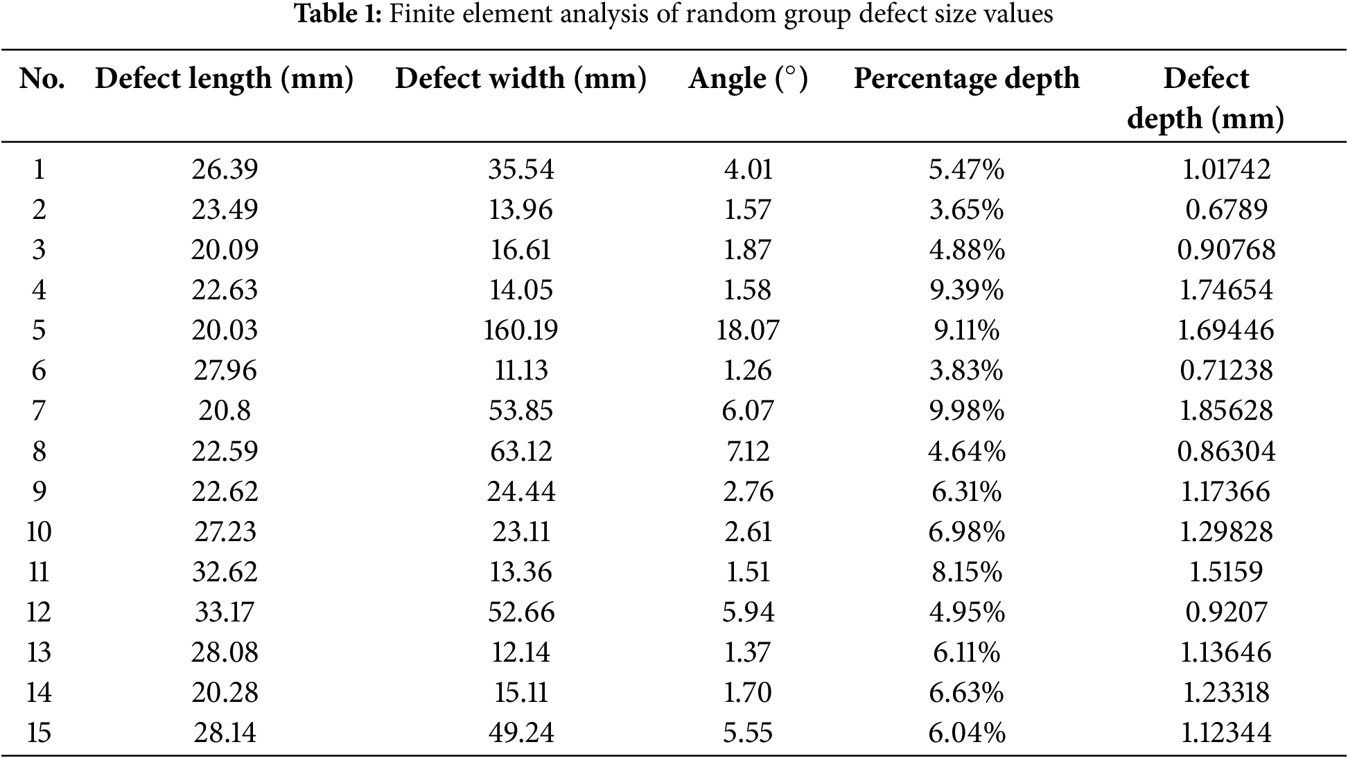
This investigation conducted an in-depth statistical analysis of magnetic flux leakage (MFL) inspection data from the Yichang-Qianjiang section of the Sichuan-East Gas Pipeline in 2023, examining three aspects: corrosion defect length, width, and depth. Through fitting the inspection data, the study determined that:

The defect length conforms to a Gamma distribution, with the probability density function:

f(x;7.52,2.18)=12.187.52Γ(7.52)x6.52e−x2.18+10(1)

where Γ(α) represents the gamma function.

The defect width follows an exponential distribution, with the probability density function:

f(x;25.5)=e−x25.525.5+10(2)

The defect depth percentage adheres to a Beta distribution:

f(x;4.4,14.2)=Γ(18.6)Γ(4.4)Γ(14.2)x3.4(1−x)13.2(3)

The statistical distributions derived from the 2023 MFL inspection data demonstrate strong alignment with actual corrosion patterns observed in long-distance gas pipelines. Analysis of the 389 detected defects revealed that 82% of defects follow these distributions, with the Gamma distribution for length reflecting the tendency of corrosion to spread longitudinally, the exponential distribution for width capturing the typical circumferential growth patterns, and the Beta distribution for depth ratio accurately representing the predominantly shallow nature of early-stage corrosion defects.

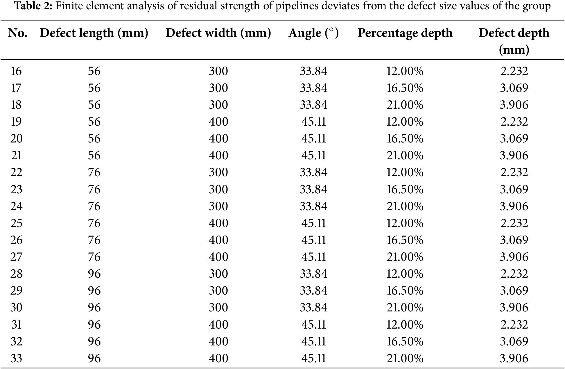
However, historical pipeline failure data from the China Pipeline Network Corporation indicates that catastrophic failures often involve defect dimensions that deviate significantly from these typical distributions, particularly in cases of accelerated corrosion or combined mechanical-chemical damage. To account for these critical scenarios, we established the deviation group with parameters deliberately selected to represent the upper 95th percentile of defect dimensions observed in historical failure cases. For example, the selected width range of 300–400 mm corresponds to documented cases where extensive circumferential corrosion led to pipeline failures in similar X70 grade pipelines. Similarly, the depth percentages (12%–21%) were chosen based on recorded failure incidents where rapid corrosion penetration occurred. This approach ensures our analysis encompasses both typical corrosion patterns and more severe scenarios that pose significant risks to pipeline integrity.

Based on these distribution functions, 15 sets of statistically consistent defect parameters were generated randomly for further analysis and validation. Each parameter set encompasses defect length, width, and depth ratio (depth percentage), presented as random groups in Table 1.

To explore the impact of defects under extreme conditions on pipeline safety more thoroughly, parameter sets deliberately deviating from the high-frequency regions of these distributions were selected, forming a “deviation group”. These parameters represent anomalous defect scenarios that diverge from normal distribution ranges, documented in Table 2.

2.1.2 Simulation Parameters Based on Influencing Factors

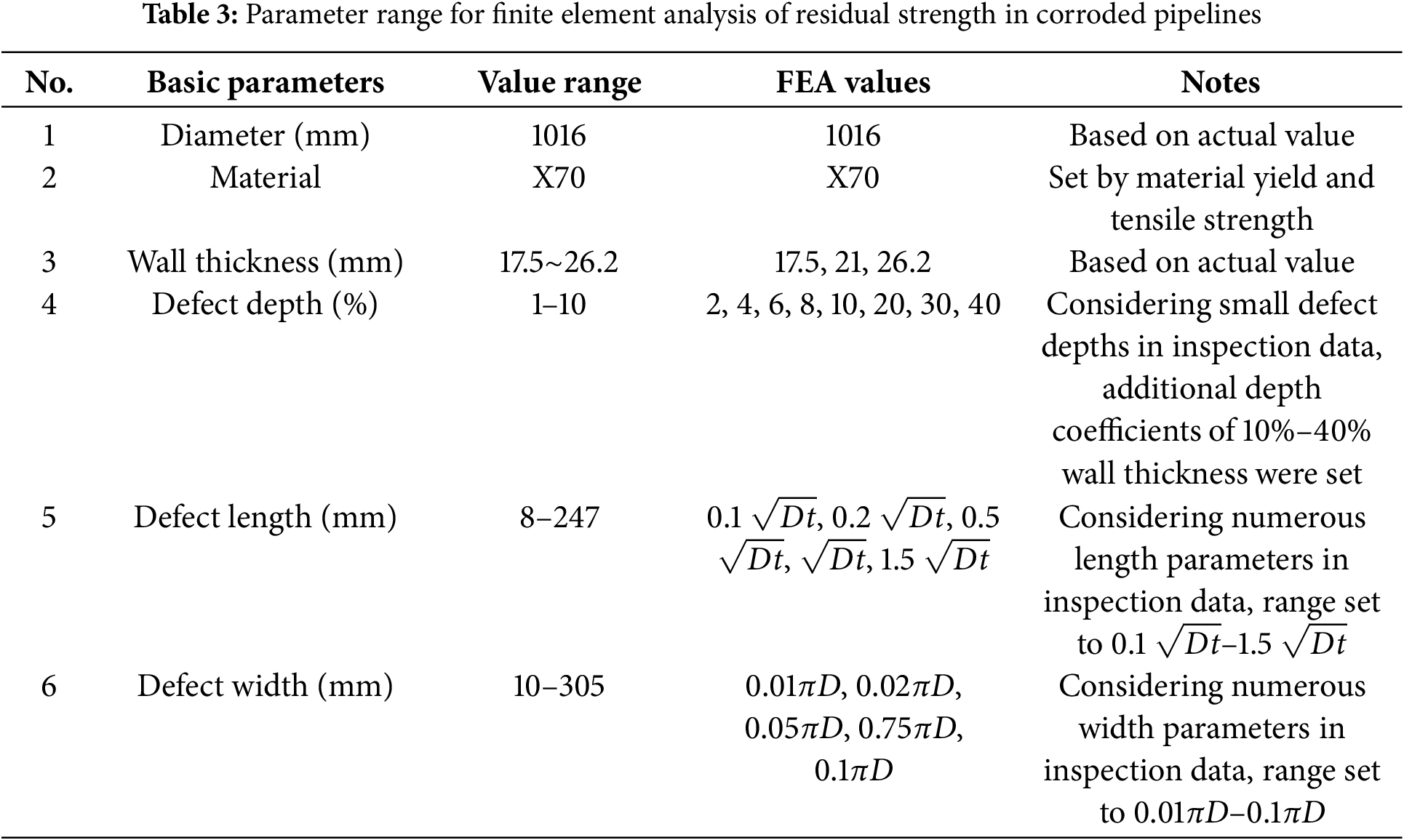
When developing machine learning models based on pipeline defect statistical analysis results, excessive reliance on existing data parameter settings may lead to overfitting issues. Overfitting indicates superior model performance on training data but poor predictive capability for new, unknown data, which evidently compromises model generalization. Therefore, to prevent overfitting and enhance model performance in practical applications, parameter setting diversity and rationality must be thoroughly considered during training, establishing broader finite element simulation parameter value ranges. Table 3 outlines the expanded parameter value ranges, which are more extensive than the original statistical results and encompass various operating conditions potentially experienced by pipelines, thereby strengthening model robustness and adaptability.

According to the defect simulation parameter settings and referencing four key factors (defect length, width, depth percentage, and circumferential angle) and the mixed-level standard orthogonal table L64 (25·410·84), 48 simulation parameter sets were established, designated as the structural group, as shown in Table 4.

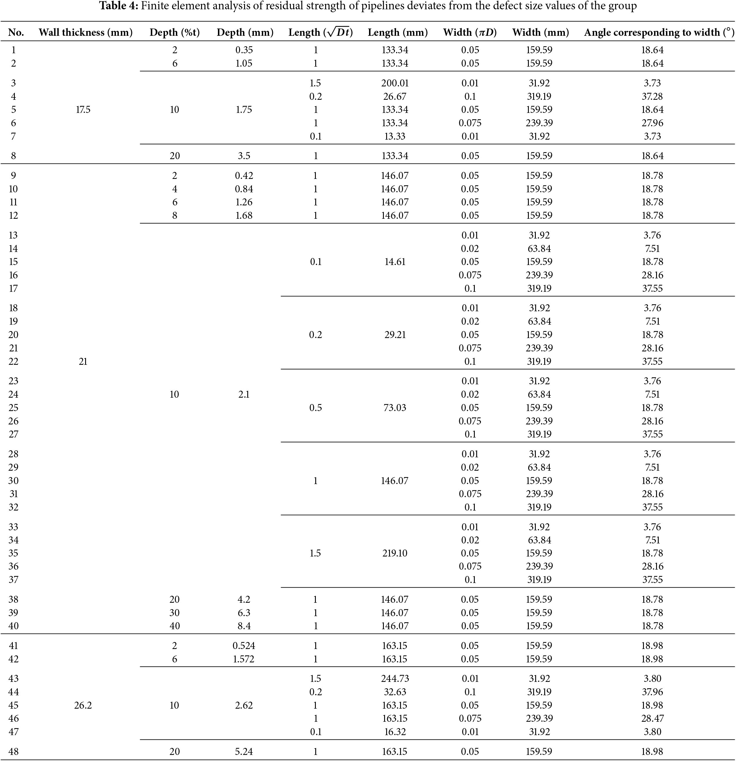
In these simulation parameters, defect depth is expressed as wall thickness percentage, while defect length and width are represented as n times Dt. Consequently, an additional set of unified simulation parameters was introduced, expressing defect length, width, and depth in absolute values to compare the effects of defect values under different wall thickness conditions, designated as the non-proportional group, detailed in Table 5. In this parameter set, defect depths are 0.84 mm, 2.1 mm, and 4.2 mm, encompassing shallow, medium, and deep defects; defect dimensions are set at 219.10 mm × 31.92 mm, 29.21 mm × 319.19 mm, and 146.07 mm × 159.59 mm, considering long defects, wide defects, and square defects, respectively.

2.2 Finite Element Model Development

2.2.1 D Modeling and Mesh Division

A three-dimensional finite element model was established using ABAQUS to simulate the corrosion-damaged pipeline. The model featured a steel pipe with internal corrosion defects, with both ends hinged and internal pressure applied to the inner surface. The relevant geometric modeling situation is shown in Table 6.

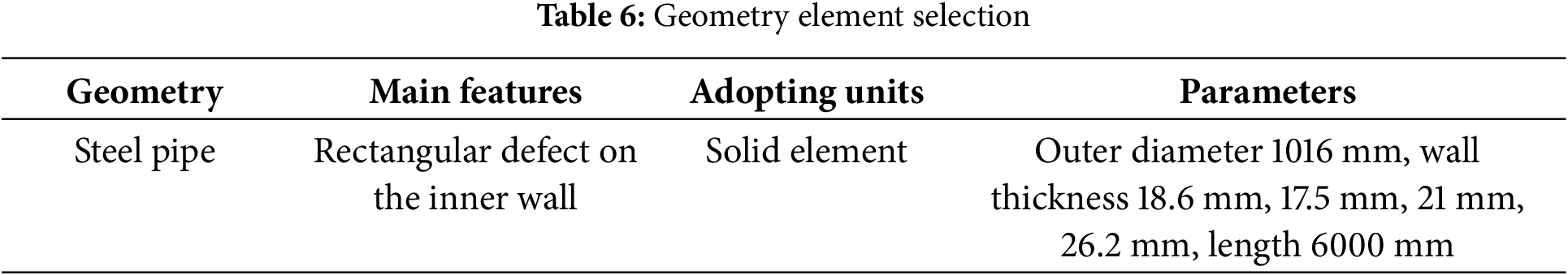
The modeling of steel pipes mainly considers the straight pipe section, which contains internal circumferential rectangular defects. Considering that the research problem is a pressure explosion problem, solid element modeling is adopted. The parameters of the pipeline include one diameter and four wall thicknesses. Specific pipeline parameters and defect sizes have been introduced in Section 2.1.

The hexahedral mesh offers several advantages, including high accuracy, good numerical stability, ease of generation, and wide applicability, making it one of the commonly used discretization models in engineering applications and providing robust support for solving various engineering problems. Therefore, this study employs hexahedral mesh with highly refined local mesh density, particularly in defect regions, and moderately refined mesh density in areas adjacent to defects, as illustrated in Fig. 1.

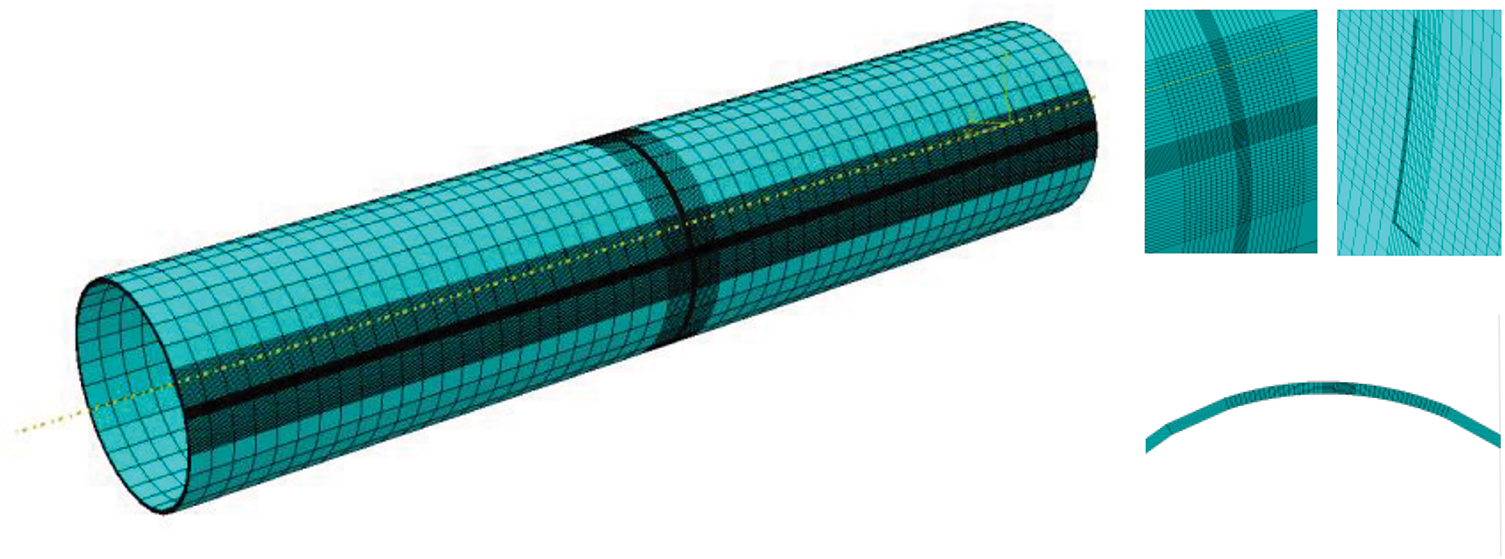
Figure 1: Mesh division

2.2.2 Material Parameter Settings

The hardening effect of materials significantly influences pipeline burst failure. To characterize the post-yield hardening behavior of pipeline materials, the Ramberg-Osgood (R-O) power hardening stress-strain relationship is generally implemented in the computational model.

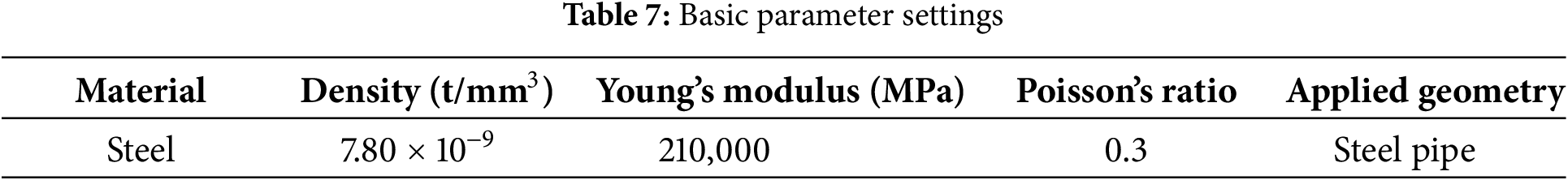
Based on the research entity, the material configuration primarily encompasses steel pipe materials, with parameters specified in Table 7 and plastic parameters detailed in Table 8. The steel pipe incorporates ductile damage with a fracture strain of 0.25, triaxial stress of 1.35, strain ratio of 1, and damage evolution displacement of 0.05.

2.2.3 Load and Boundary Conditions

Internal pressure is applied to the pipeline inner wall within the Load module. This internal pressure generates a compressive load P on the steel pipe’s inner surface, as illustrated in Fig. 2. This design considers the mechanical characteristics during the burst process, implementing burst through internal pressure application. Specifically, internal pressure increases gradually from 0 to 100 MPa over 1 s, as demonstrated in Fig. 3.

Figure 2: Loading conditions

Figure 3: Internal pressure loading method

To maintain zero overall degrees of freedom and prevent unnecessary displacement or deformation during the repair process, fixed boundary conditions are established at both ends of the steel pipe. These fixed boundary conditions effectively constrain the pipe’s range of motion.

Additionally, boundary conditions preventing longitudinal displacement are implemented at both pipe ends, as shown in Fig. 4. This configuration ensures the pipe maintains a fixed length during the burst process, preventing longitudinal displacement. Such boundary conditions preserve the pipe’s original length while preventing unnecessary stress and deformation caused by displacement.

Figure 4: Boundary conditions

2.2.4 Solving Calculation

Considering the physical process of steel pipe burst involving substantial deformation, this aspect requires thorough consideration in numerical simulation. In actual burst processes, the pressurization phase proceeds gradually, while the burst phase occurs within an extremely brief duration. To accurately simulate this process, this research implements dynamic implicit analysis steps in ABAQUS software, utilizing the Newton-Raphson algorithm to solve equilibrium equations with geometric nonlinearity enabled. The force convergence criterion serves as the convergence standard, and the total simulation duration extends to 5 s.

2.2.5 Failure Criteria

Pipeline failure pressure denotes the pressure threshold at or above which leakage or rupture incidents materialize. Stress failure criteria represent the most universal standard for determining corrosion pipeline failure pressure Fig. 5. Three widely adopted criteria include: 1) elastic failure criterion; 2) plastic limit state failure criterion; and 3) plastic failure criterion.

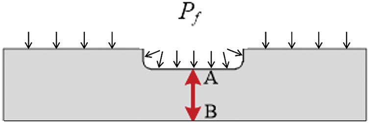
Figure 5: Schematic diagram of corrosion defect failure determination

Given the favorable ductility of oil and gas pipeline materials, comprehensive analysis suggests the plastic failure criterion proves most rational. The failure criterion based on von Mises equivalent stress at individual nodes in defect regions exhibits high sensitivity to mesh refinement, whereas the method examining equivalent stress across all nodes along the wall thickness direction in defect regions demonstrates lower mesh precision requirements. Therefore, for corrosion defects, this research’s failure criterion examines the stress state along the wall line. Failure occurs when equivalent stress at all nodes along line AB reaches the material’s ultimate tensile strength, with the corresponding internal pressure representing the residual strength (failure pressure) of the corroded pipeline.

To enhance simulation accuracy and stability, this research employs an incremental step approach. The initial increment step encompasses 0.005 s, ensuring gradual introduction of larger deformations and stresses during simulation. Additionally, a maximum increment step of 0.5 s maintains simulation stability.

Acknowledging the extremely brief nature of the burst process, this study establishes a minimum increment step of 0.0000000001 s to facilitate numerical convergence. This configuration ensures sufficiently small time steps during simulation to capture rapid changes and high-frequency vibrations potentially emerging during the burst phase. Such time step settings enable more precise simulation of physical behaviors and responses during the steel pipe burst process.

2.3 Theoretical Foundation

The residual strength assessment of corroded pipelines fundamentally relies on fracture mechanics principles and elastic-plastic theory. The primary theoretical framework encompasses three key aspects: stress distribution analysis, failure criteria development, and burst pressure prediction.

2.3.1 Stress Distribution Theory

For a cylindrical pipeline subject to internal pressure P, the hoop stress σθ and axial stress σZ in the pipe wall can be expressed as:

σθ=PD2t(4)

σZ=PD4t(5)

where D is the pipe diameter and t is the wall thickness. However, in the presence of corrosion defects, stress concentration occurs and the local stress field becomes more complex. The stress concentration factor K at the defect region can be approximated by:

K=1+2dt(6)

where d is the defect depth. This relationship explains our experimental observation of accelerated strength reduction with increasing defect depth.

2.3.2 Failure Criteria Development

The failure of corroded pipelines typically follows the von Mises yield criterion:

σ12+σ22+σ32−σ1σ2−σ2σ3−σ3σ1=σy(7)

where σ1, σ2, and σ3 are principal stresses and σy is the yield strength. For complex defect geometries, the effective stress σeff must account for both membrane and bending stresses:

σeff=(σm2+3τ2)(8)

where σm is the membrane stress and τ is the shear stress.

2.3.3 Burst Pressure Prediction Model

Based on these theoretical foundations, the burst pressure Pb for a corroded pipeline can be predicted using:

Pb=2t⋅σu⋅MD−tM(9)

where σu is the ultimate tensile strength and M is the Folias factor:

M=11+0.8L2Dt(10)

where L is the defect length. This theoretical framework explains our experimental findings regarding the relationship between defect dimensions and residual strength, particularly the observed 0.054 MPa reduction in strength per millimeter increase in defect depth.

3  Experimental Validation

3.1 Experimental Design

To validate the reliability of finite element simulation and accuracy of the prediction model, this research conducts hydraulic burst experiments on corroded pipelines to evaluate their ultimate pressure-bearing capacity. The experiments primarily focus on commonly encountered pipelines with a diameter of 1016 mm, corresponding to the actual dimensions of the West-East Gas Pipeline. Given the substantial pressure requirements and experimental scale of full-size tests, coupled with facility and safety constraints, this study implements a scaled model approach.

The experimental model features an external diameter of 80 mm, scaled at 1:12.7 from the prototype pipeline diameter of 1016 mm. The scaled model utilizes identical material properties as the prototype, with elastic modulus E = 207 GPa, yield strength σs = 565 MPa, and density 7.85 g/cm3. As stress scaling remains independent of length, and the scaled model comprises the same material as the prototype, their pressure-bearing capacities remain equivalent, resulting in identical burst pressures. Table 9 presents the scaled model parameters.

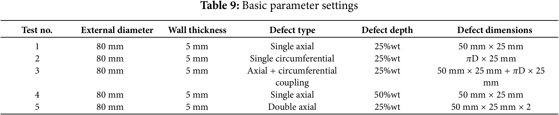
Post-acquisition processing of experimental pipes requires several steps. For pipes with anti-corrosive coating, sandblasting removes the protective layer until complete pipe exposure, followed by machining to fabricate pre-designed corrosion defects. Upon completion of defect fabrication, standard elliptical heads are welded to both pipe ends to form sealed vessels. The head specifications reference GB/T 25198–2010 “Pressure Vessel Heads,” with 100% radiographic examination of circumferential welds connecting heads and pipe specimens according to JB/T 4730.3-2005 “Non-destructive Testing of Pressure Equipment” Level II. A pressure connection port integrates into the center of one elliptical head, while the opposite end incorporates a vent for air evacuation during water filling.

The burst experiment employs water as the pressurizing medium, conducted in a SUP-BPXT-300 hydraulic testing machine. Instrumentation measures parameters including pressure and water intake volume to obtain data on depressurization behavior, crack propagation velocity, and temperature during burst testing. Pressure measurement utilizes a precision gauge with 40 MPa range and 0.4% accuracy. Water intake measurement employs an E + H80F mass flowmeter featuring 0.25% accuracy and 0.1 mL minimum scale division.

3.2 Experimental Procedure

The experimental protocol encompasses the following sequential phases:

(1) Preparation of experimental steel pipes with pre-fabricated defects, simulating corrosion damage in the Sichuan-East Gas Pipeline;

(2) Horizontal positioning of the pipeline with defects oriented upward, followed by end cap welding and circumferential weld quality inspection. Subsequently, installation of instrumentation and measuring devices;

(3) Implementation of vessel pressure-burst testing system utilizing water as the medium. Upon system connection, multiple pressure cycling operations eliminate residual air within specimens while simultaneously verifying system hermeticity and validating instrument/sensor functionality and measurement accuracy;

(4) Application of stepwise pressurization methodology. At lower pressure ranges, gradual pressure elevation proceeds with fixed water intake volumes serving as control benchmarks for each pressure gradient. Each pressure plateau maintains consistent pressure while recording water intake volume and strain data;

(5) Initiation of burst testing upon exceeding design pressure. Below yield pressure, measurements of water intake volume and strain utilize intermittent pump cessation methodology. Upon observation of specimen yielding, continuous pressurization proceeds without interruption until specimen rupture;

(6) Continuous monitoring and recording of pressure gauge data throughout the experimental duration;

(7) Post-experimental site remediation.

4  Results and Discussion

4.1 Finite Element Simulation Results and Discussion

4.1.1 Pipeline Burst Evolution Process

From the deviation group featuring larger defect dimensions, case 28 was selected to analyze the pressure-bearing burst process of defective pipelines, as illustrated in Fig. 6. The process initiates with overall stress concentration at the defect location, followed by intensified stress concentration at both circumferential edges of the defect. As plastic strain develops to a certain extent, one edge ruptures, while the stress release on this side prevents rupture of the opposite edge. Subsequently, the crack propagates rapidly along the longitudinal direction of the pipeline within an extremely brief duration.

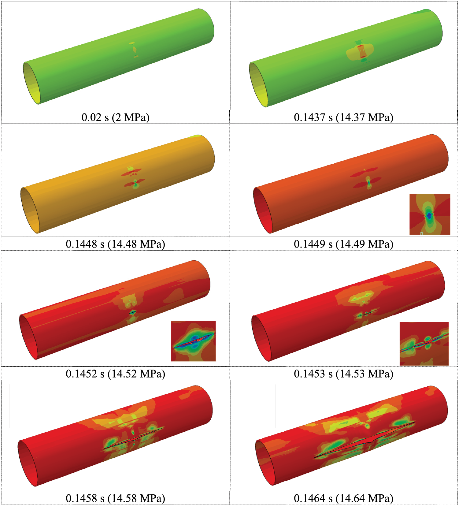
Figure 6: Stress distribution during burst process of deviation group case 28 defective pipeline

From the random group with smaller defect dimensions, case 8 was selected for analysis, as shown in Fig. 7. The process begins with overall stress concentration at the defect location, progressing to rupture once plastic strain reaches a critical level, followed by rapid longitudinal crack propagation.

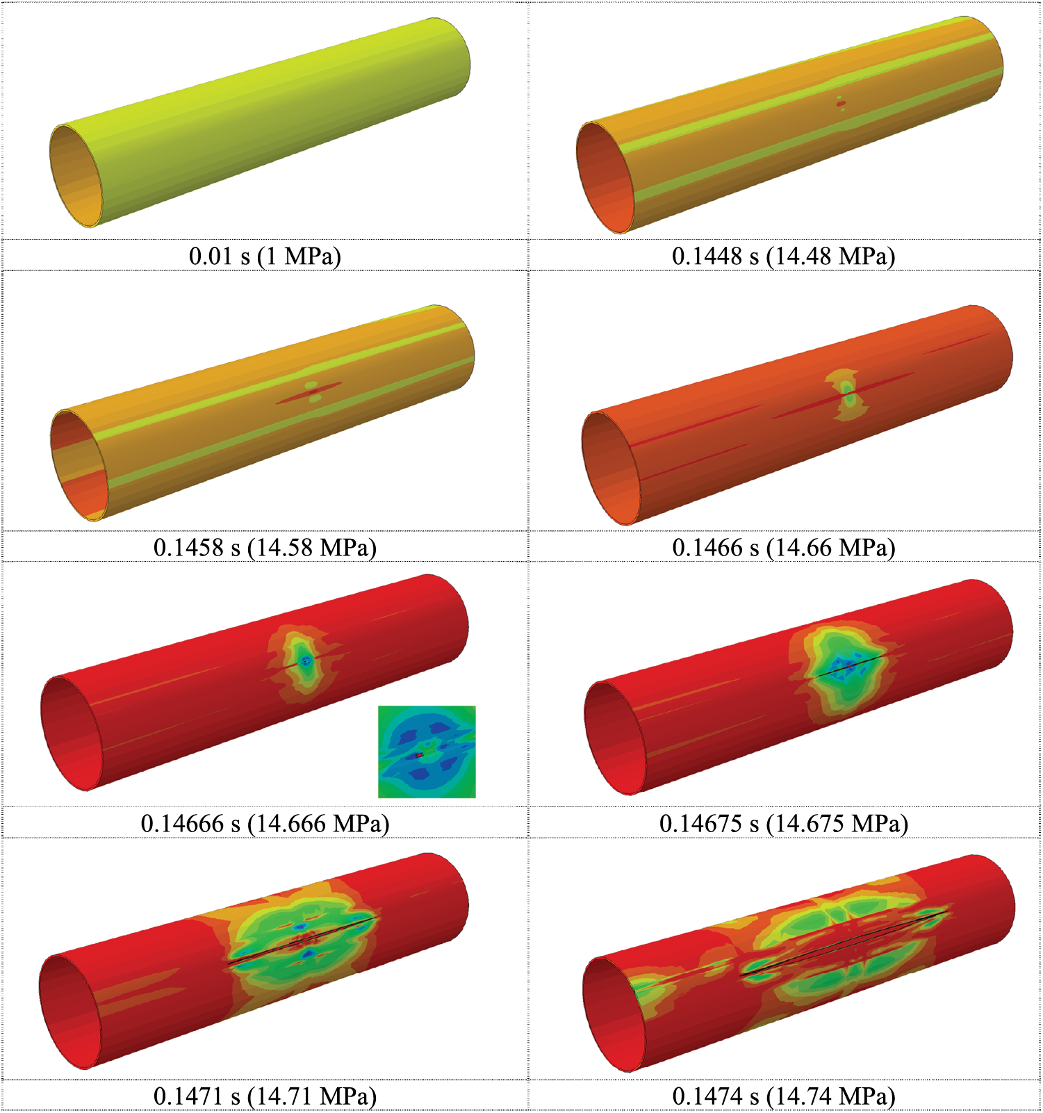
Figure 7: Stress distribution during burst process of random group case 8 defective pipeline

Fig. 8 presents stress distribution contours at the inner wall defect during the burst process for both deviation group case 28 and random group case 8. The key distinction between large and small defects lies in their stress concentration patterns: large defects exhibit final stress concentration at the upper and lower circumferential edges, initiating cracks from these edges with longitudinal propagation. Conversely, small defects concentrate stress in their center, resulting in central crack initiation with longitudinal development.

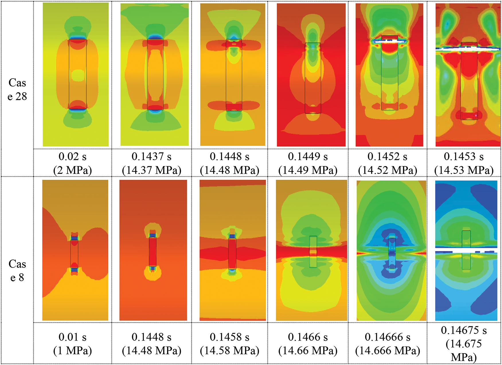
Figure 8: Defect stress distribution during burst process for deviation group case 28 and case 8

Simulation results from both random and deviation groups reveal characteristic failure patterns under typical conditions. Regardless of defect size, pipeline failure manifests longitudinally when plastic strain develops under pressure, with rapid longitudinal propagation.

4.1.2 Burst Crack Morphology in Corroded Pipelines

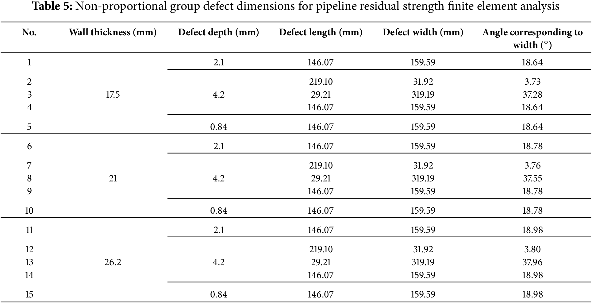
To comprehensively evaluate the influence of corrosion defects on pipeline burst behavior, select cases from both structural and non-proportional groups were analyzed for post-burst crack morphology.

Burst Crack Patterns under Various Defect Lengths

In the structural group, pipelines with 21 mm wall thickness were selected to analyze crack morphology differences among cases 7, 12, 17, 22, and 27. These cases correspond to scenarios with 10% wall thickness depth, 0.05πD width, and lengths of 0.1 Dt, 0.2 Dt, 0.5 Dt, Dt, 1.5 Dt, respectively, as depicted in Fig. 9.

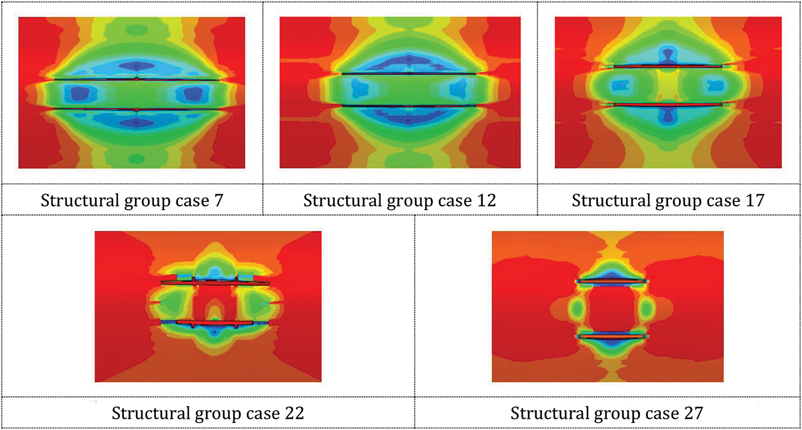
Figure 9: Pipeline burst crack patterns under different defect lengths

Fig. 9 illustrates stress distributions at inner wall defects during burst for varying defect lengths. Notable observations indicate that burst pressure diminishes progressively with increasing defect length. Initial crack dimensions at burst initiation exhibit inverse relationships with defect length: crack length decreases while width increases as defect length grows. This phenomenon occurs because shorter defects minimally impact pipeline strength uniformity, resulting in more gradual, slender longitudinal cracks at burst pressure. Conversely, longer corrosion defects significantly reduce localized pipeline strength, leading to more abrupt crack formation.

Burst Crack Patterns under Various Defect Depths

Analysis of cases 1–4, 22, and 30–32 from the structural group with 21 mm wall thickness examined scenarios with defect length of Dt, width of 0.05πD, and depths ranging from 2% to 40% wall thickness (2%, 4%, 6%, 8%, 10%, 20%, 30%, 40%), as shown in Fig. 10.

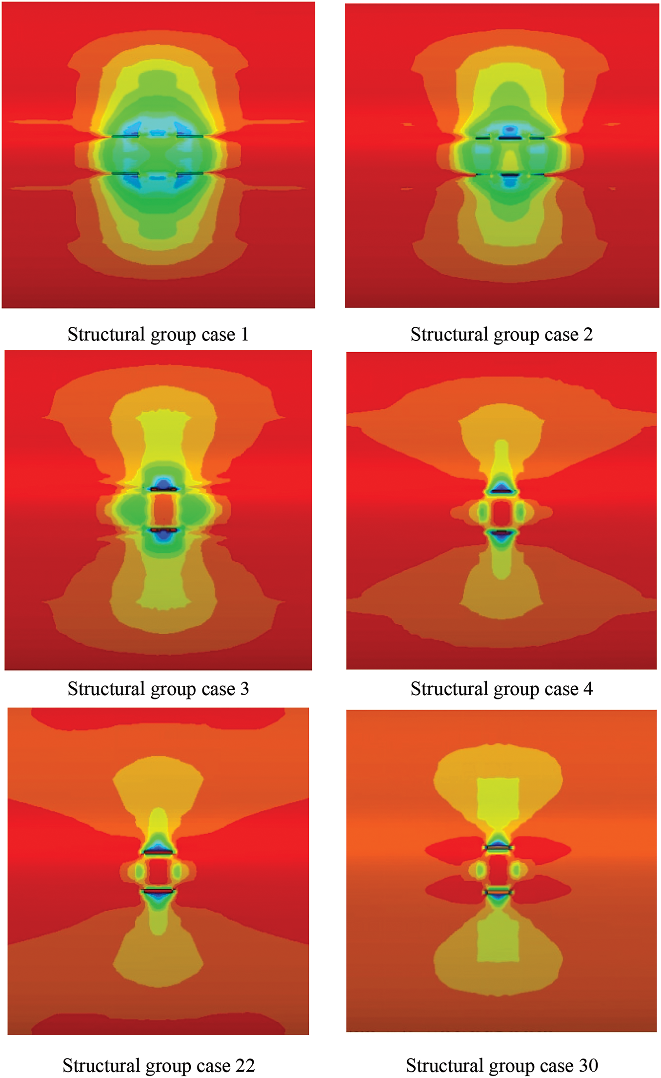
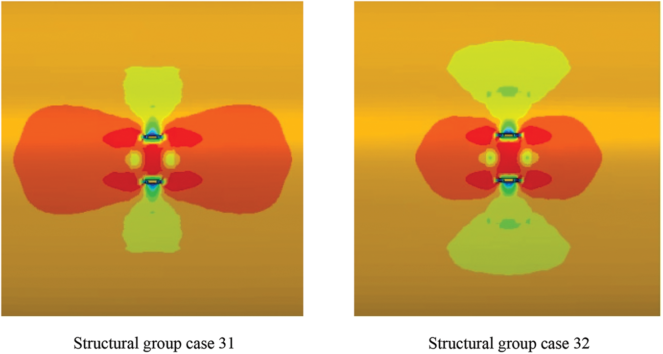
Figure 10: Pipeline burst cracks under different defect depths

Fig. 10 presents stress distributions for varying defect depths. Results demonstrate progressive reduction in burst pressure with increasing defect depth. Initial crack characteristics at burst onset show dimensional relationships with defect depth: crack length decreases while width increases with greater depth. Shallow defects (2%–6%) initiate cracks from four corners with axial development, while deeper defects generate cracks from axial edge centers with subsequent axial propagation.

Burst Crack Patterns under Various Defect Widths

Analysis of cases 5–9 from the structural group with 21 mm wall thickness examined crack morphology variations with defect length of 0.1Dt, depth of 10%, and widths ranging from 0.01πD to 0.1πD (0.01πD, 0.02πD, 0.05πD, 0.075πD, 0.1πD), as illustrated in Fig. 11.

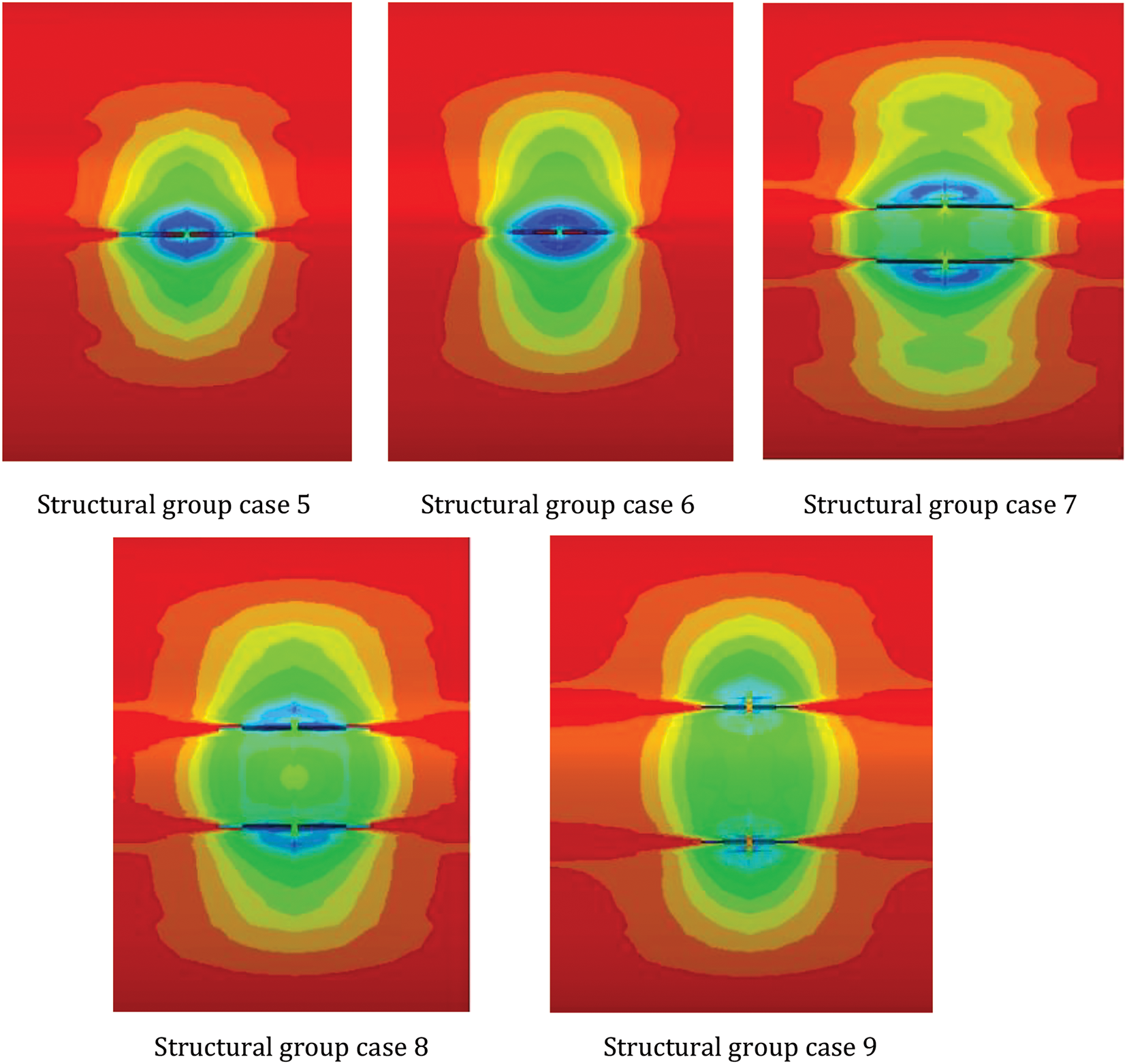
Figure 11: Pipeline burst cracks under different defect widths

Fig. 11 depicts stress distributions at inner wall defects during burst for varying defect widths. Observations reveal that as width increases, burst crack patterns evolve from single to double cracks. For defect widths below 0.05πD, cracks initiate at the defect center. When defect width exceeds 0.05πD, cracks originate at four corners, initially propagating along the outer sides of the axial ends before extending toward the pipeline center.

Burst Crack Patterns under Various Wall Thicknesses

Comparative analysis involved case 8 (17.5 mm wall thickness), case 30 (21 mm wall thickness), and case 8 (26.2 mm wall thickness) from the structural group to examine crack pattern variations under proportionally equivalent defects. All cases maintained consistent defect parameters: length of Dt, width of 0.075πD, and depth of 20%, with results shown in Fig. 12.

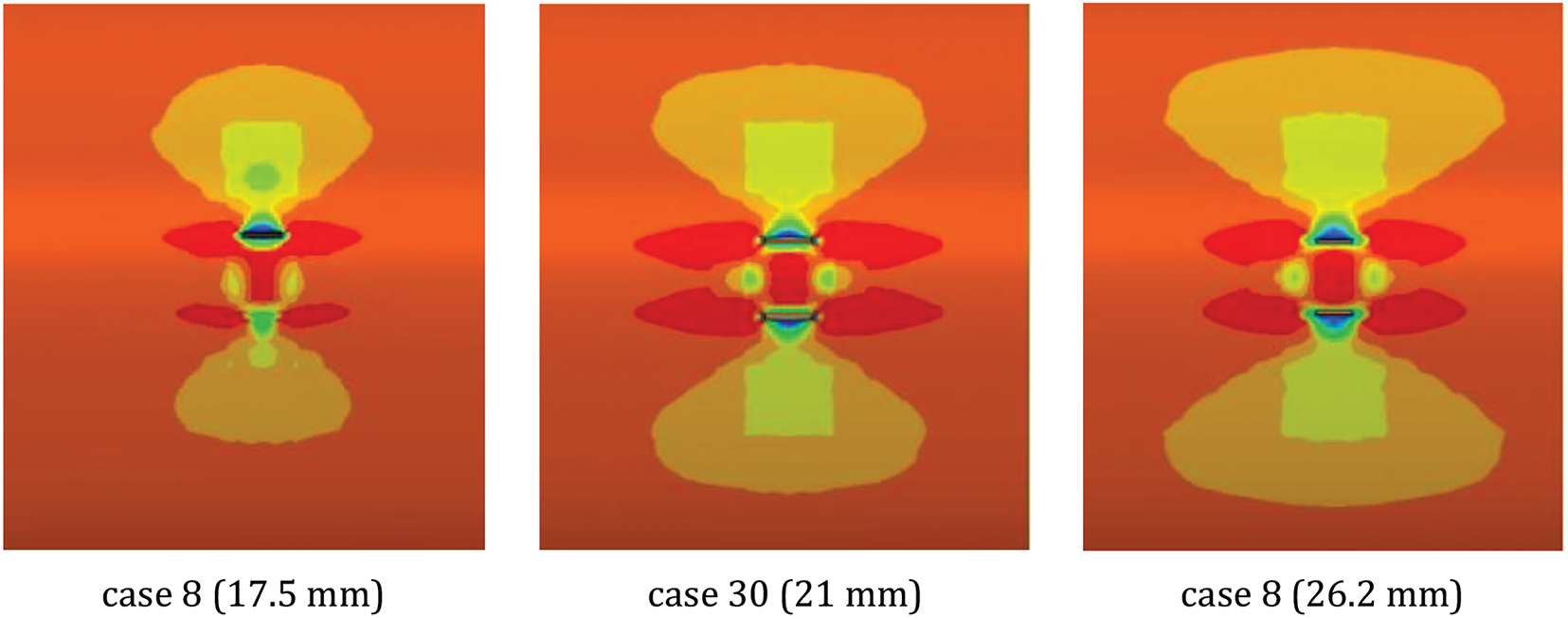
Figure 12: Pipeline burst cracks under different wall thicknesses with proportionally equivalent defects

Fig. 12 illustrates stress distributions for equivalent proportional defects across different wall thicknesses. Comparison between 17.5 mm case 8 and 21 mm case 30 reveals evolution from single to double cracks with increased width, with thicker walls more prone to double crack formation. Comparing 21 mm case 30 with 26.2 mm case 8 shows wider, shorter cracks in the latter. Combined with previous analyses, this suggests increased defect sensitivity in thicker walls when defect proportions remain constant (length as xDt, width as yπD, depth as z% wall thickness).

From the non-proportional group, cases 4, 9, and 14 were selected, corresponding to wall thicknesses of 17.5, 21, and 26.2 mm, respectively. All cases maintained uniform defect dimensions: 146.07 mm length, 159.59 mm width, and 4.2 mm depth, with results presented in Fig. 13.

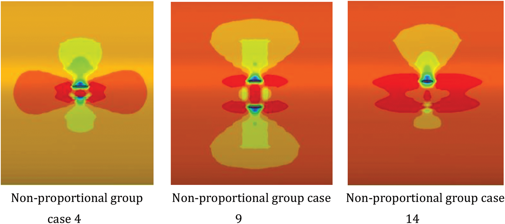
Figure 13: Pipeline burst cracks under different wall thicknesses with dimensionally equivalent defects

Fig. 13 shows stress distributions for identical defect dimensions across varying wall thicknesses. As wall thickness increases, crack patterns initially evolve to double cracks before reverting to single cracks. However, contour analysis reveals tendencies toward double crack development in all cases. In cases 4 and 14, crack formation on one side leads to stress reduction and crack arrest on the opposite side, while case 9 exhibits bilateral crack formation. Overall, failure pressure demonstrates significant enhancement with increased wall thickness. The non-linear nature of these patterns indicates complex interrelationships among failure pressure, defect dimensions (length, width, depth), and wall thickness, underscoring the significance of machine learning applications in burst pressure prediction.

4.2 Verify Experimental Results and Comparison

4.2.1 Verify Experimental Results

Burst experiments were conducted on pipelines 01–05, with their pre-test morphologies of pre-fabricated defects illustrated in Fig. 14a–e.

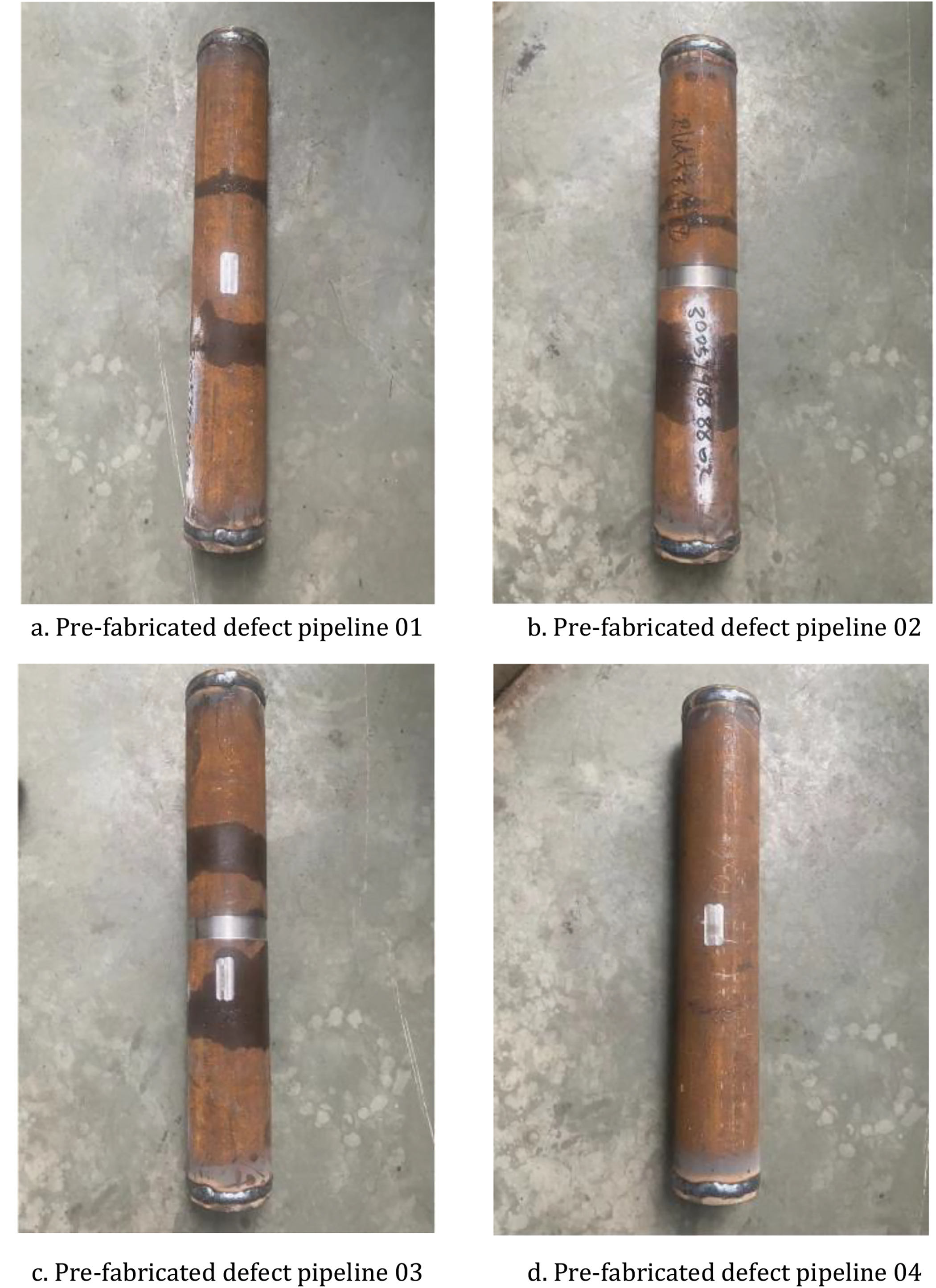
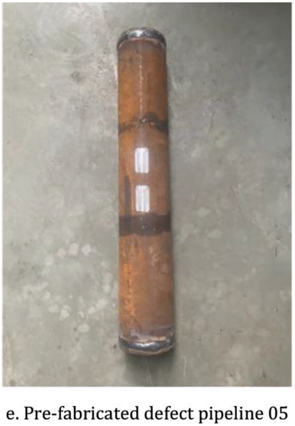
Figure 14: Pipeline morphology prior to burst testing

The experimental results for these five pipelines are presented in Table 10.

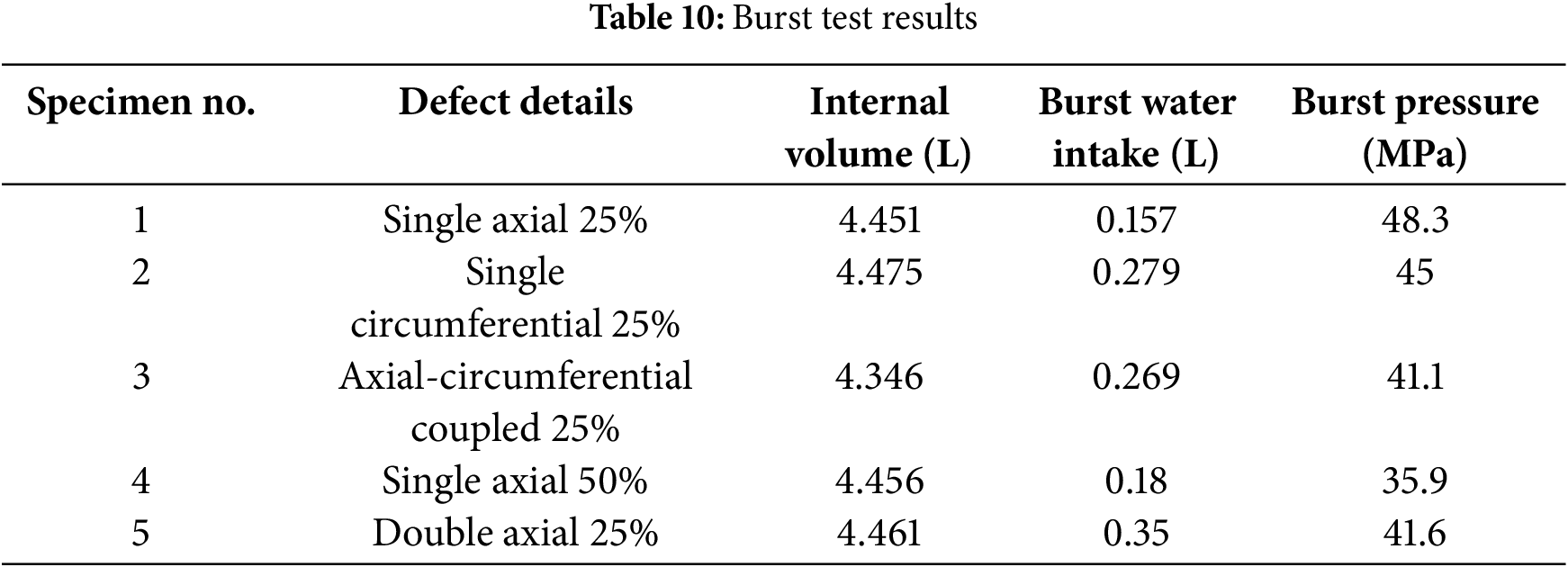
For pipeline 01, Fig. 15a demonstrates its condition during testing, Fig. 15b reveals its post-burst morphology, and Fig. 15c presents the pressure-water intake curve throughout the burst testing process.

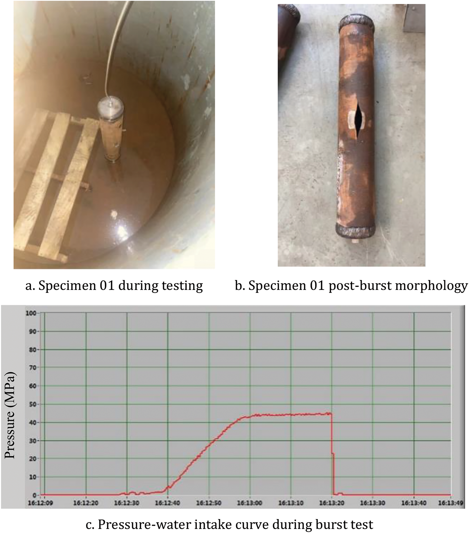
Figure 15: Pipeline 01 experimental results

For pipeline 02, Fig. 16a demonstrates its condition during testing, Fig. 16b reveals its post-burst morphology, and Fig. 16c presents the pressure-water intake curve throughout the burst testing process.

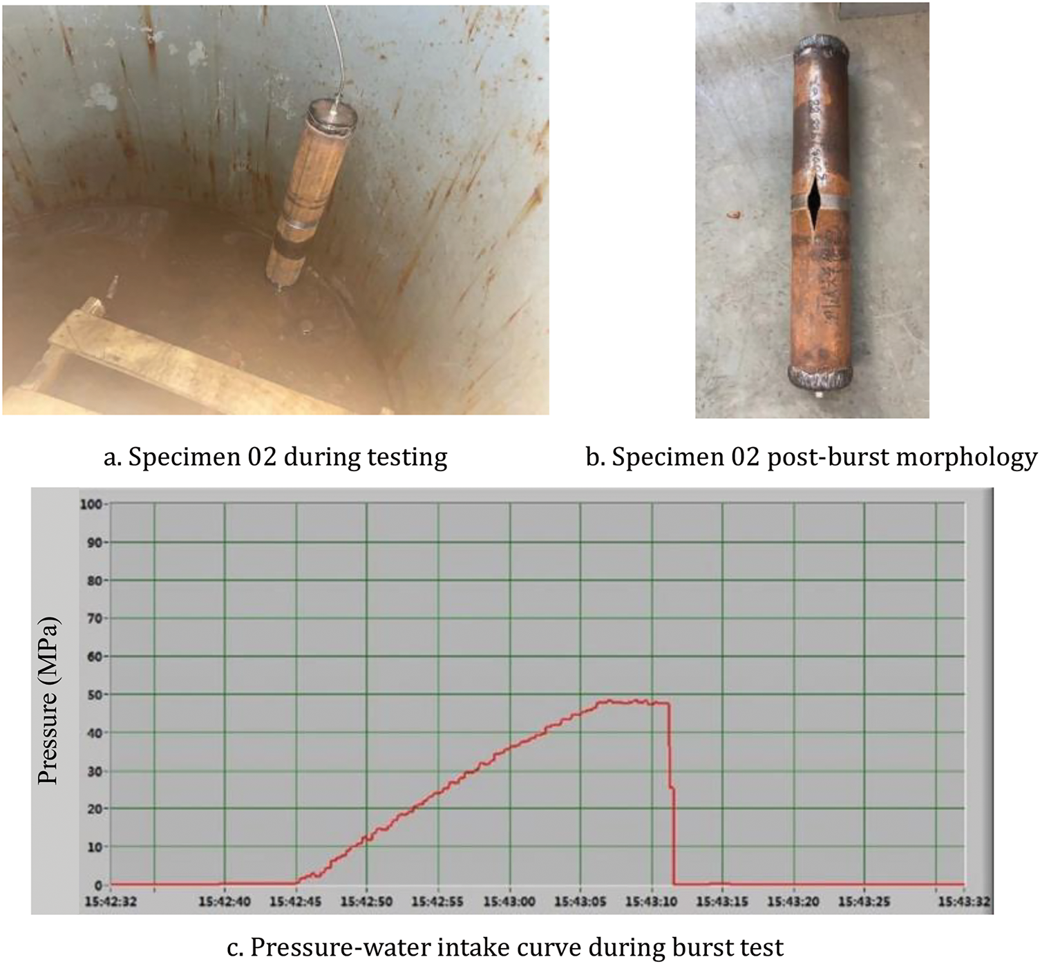
Figure 16: Pipeline 02 experimental results

For pipeline 03, Fig. 17a demonstrates its condition during testing, Fig. 17b reveals its post-burst morphology, and Fig. 17c presents the pressure-water intake curve throughout the burst testing process.

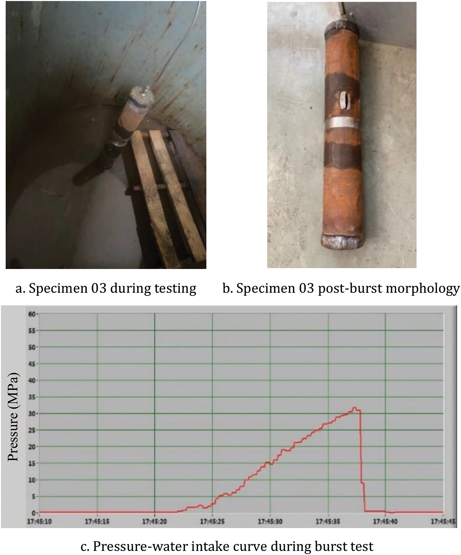
Figure 17: Pipeline 03 experimental results

For pipeline 04, Fig. 18a demonstrates its condition during testing, Fig. 18b reveals its post-burst morphology, and Fig. 18c presents the pressure-water intake curve throughout the burst testing process.

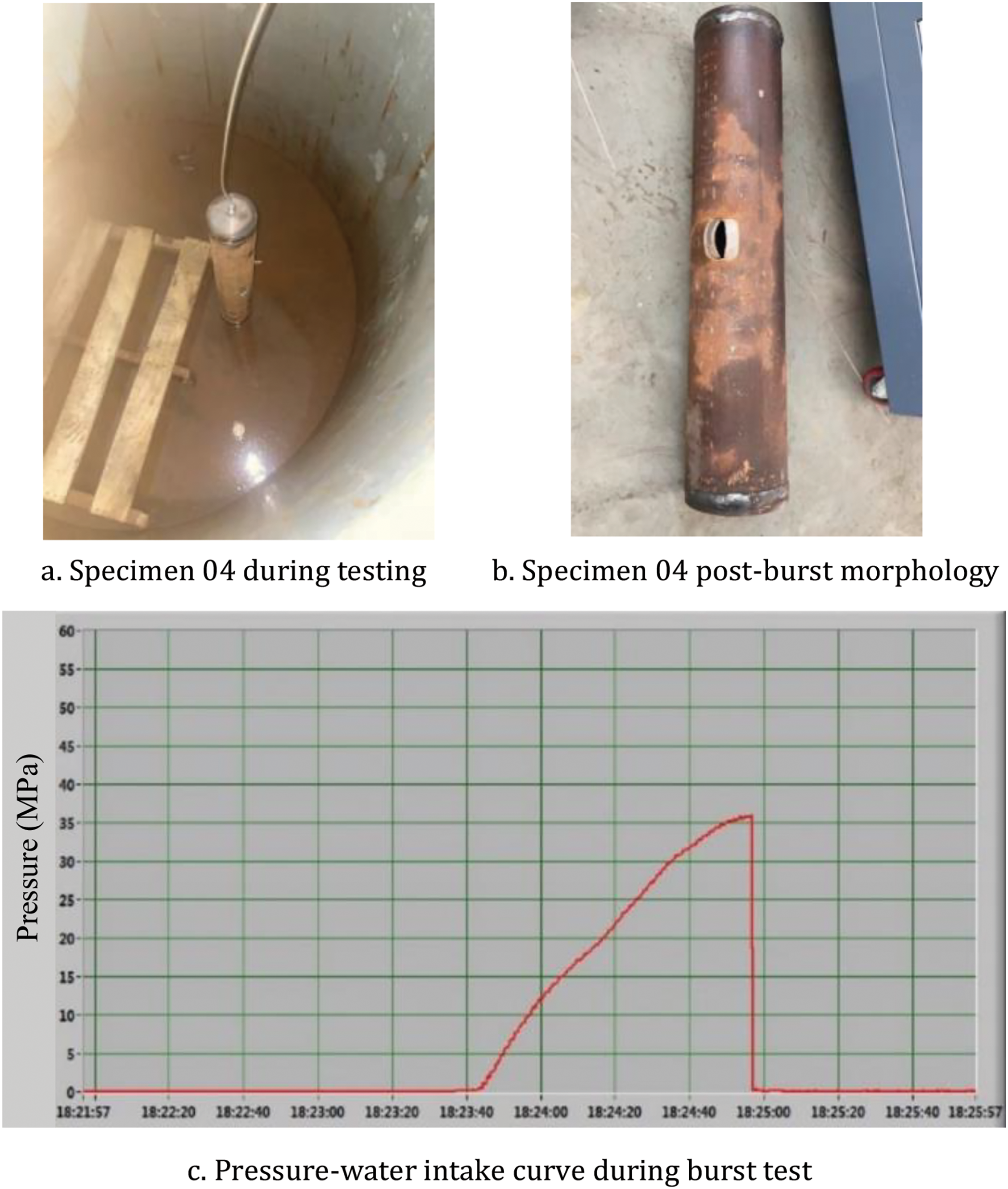
Figure 18: Pipeline 04 experimental results

For pipeline 05, Fig. 19a demonstrates its condition during testing, Fig. 19b reveals its post-burst morphology, and Fig. 19c presents the pressure-water intake curve throughout the burst testing process.

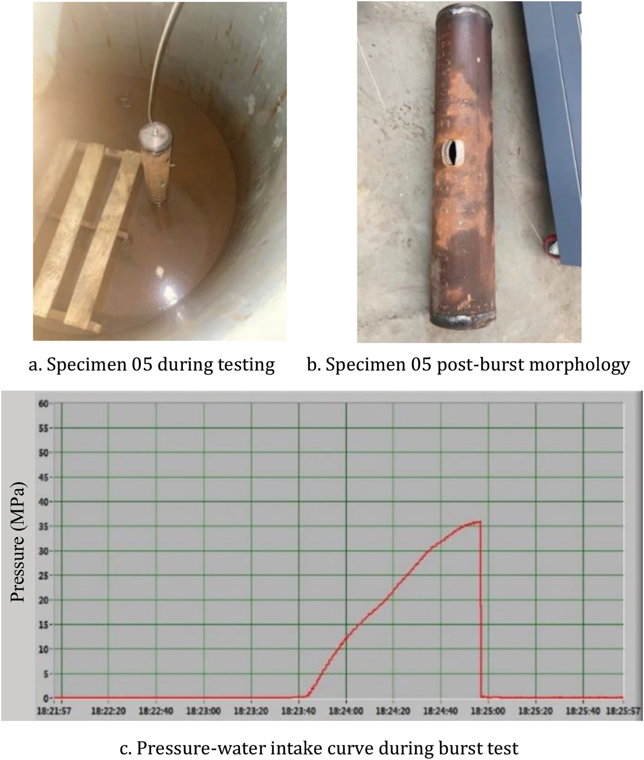
Figure 19: Pipeline 05 experimental results

4.2.2 Comparison between Experimental Results and Finite Element Calculation Results of Residual Strength of Pipelines

A comparative analysis was performed between the burst experimental results of corroded pipelines and finite element calculations of remaining strength. The finite element simulation results are illustrated in Fig. 20a–e.

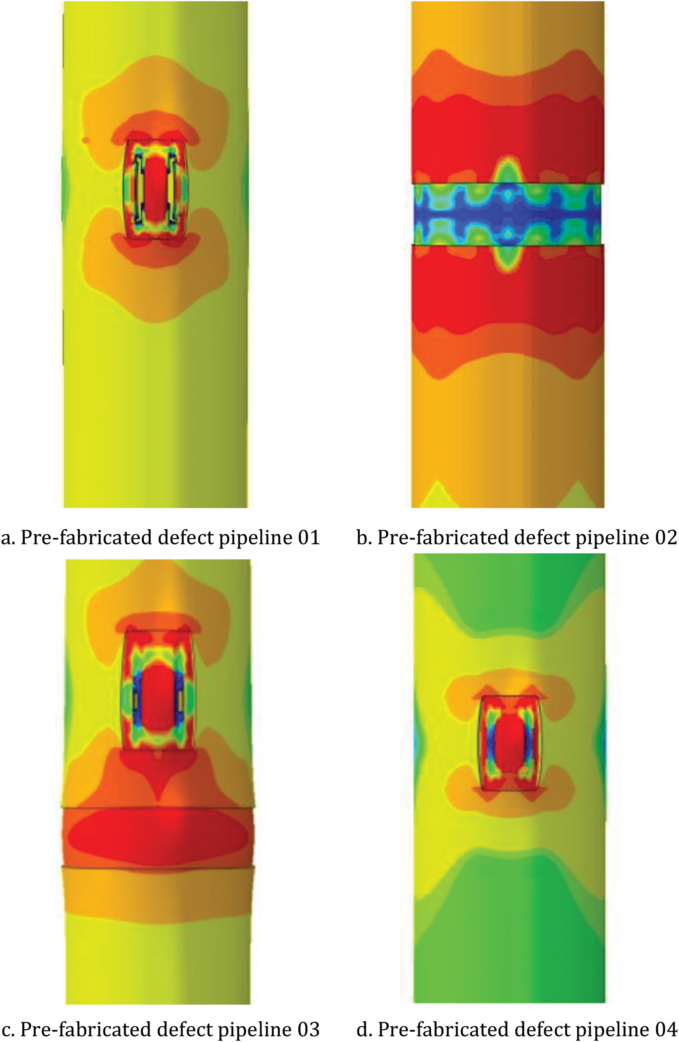
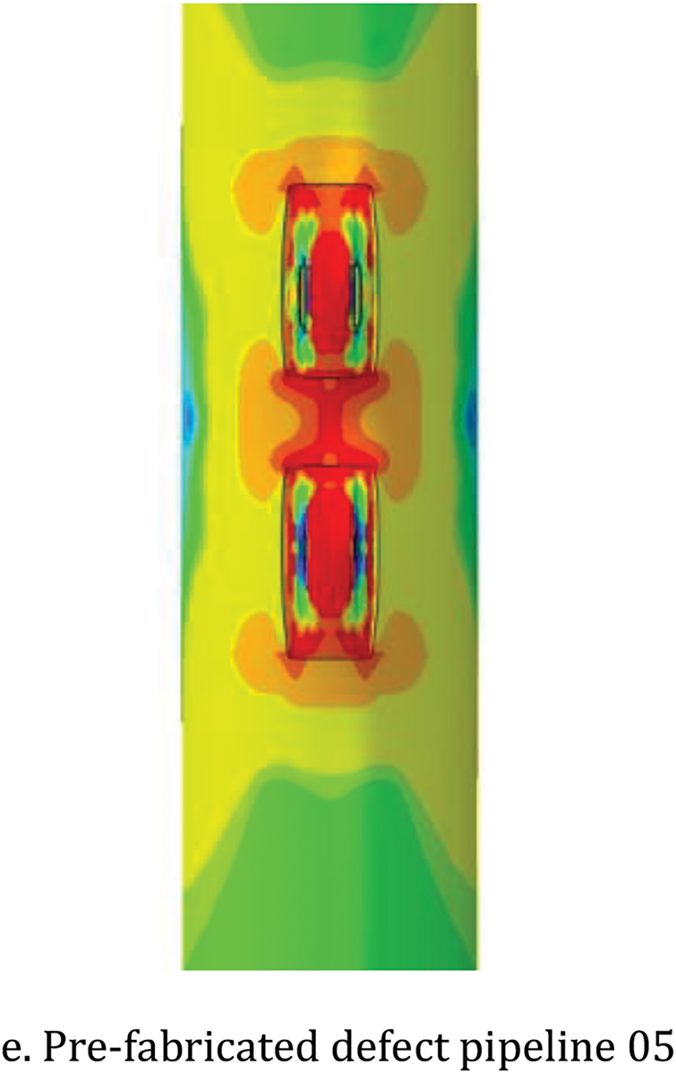
Figure 20: Finite element simulation results

Table 11 presents the comparison between experimental results and finite element simulation results.

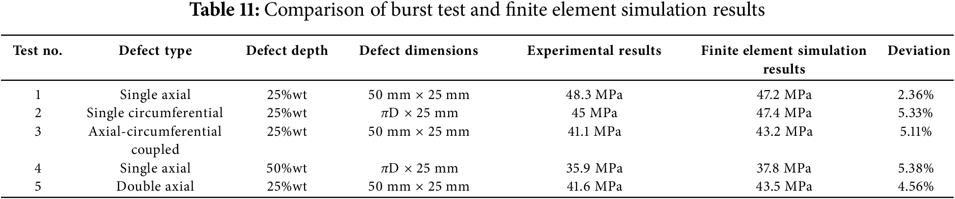
Experimental validation confirms the accuracy of finite element simulation results, with deviations consistently around 5% and reaching as low as 2.36%, indicating high reliability of the dataset established through finite element simulation.

4.2.3 Comparison of Prediction Model Calculations

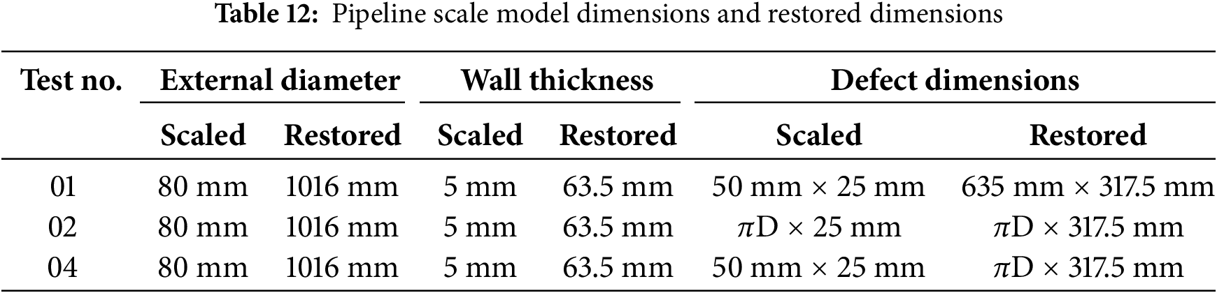
The burst test pipelines utilized scaled models. For comparison with the remaining strength prediction model, dimensions were first scaled up to 1016 mm external diameter, with other dimensional characteristics proportionally enlarged. As the prediction model addresses only single corrosion cases, comparisons were limited to experimental groups 01, 02, and 04. Table 12 presents the scaled and restored dimensions. Comparative results are presented in Table 13.

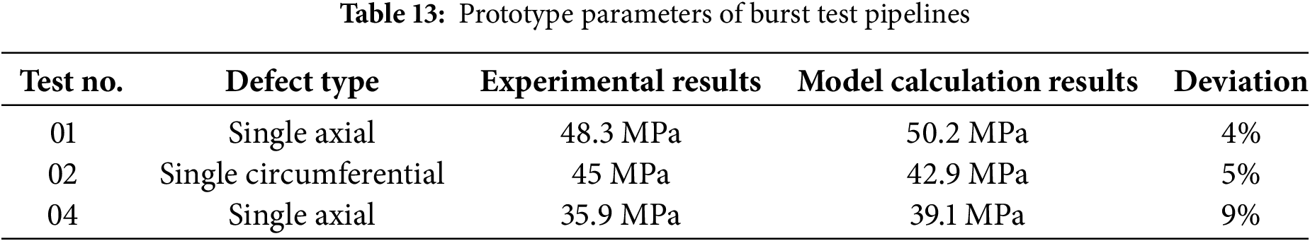
Experimental validation confirms that deviations between the remaining strength prediction model calculations and experimental measurements remain within 10%, demonstrating satisfactory accuracy of the remaining strength prediction model results.

4.2.4 Error Analysis and Model Robustness Assessment

While the overall deviation between experimental and simulation results remains within 5%, detailed error analysis reveals specific patterns in prediction accuracy. The model’s error distribution exhibits systematic variations under different conditions:

For standard defect scenarios (depth <30% wall thickness), the average deviation is 2.8%, with errors primarily stemming from idealized material property assumptions. However, as defect depth increases beyond 30%, the deviation gradually increases, reaching 4.5% at 40% wall thickness penetration. This trend suggests that deeper defects introduce additional complexity in stress distribution patterns that slightly impact model accuracy.

The model demonstrates varying sensitivity to defect geometry. For circumferential defects, prediction accuracy improves with increasing defect width, showing minimal deviation (1.9%) for defects wider than 0.05πD. Conversely, axial defects exhibit slightly higher deviations (3.2%–4.1%) as defect length increases beyond 0.5 Dt, likely due to enhanced stress concentration effects.

To evaluate model robustness under extreme scenarios, additional validation tests were conducted with three severe defect cases: (1) large-scale pitting corrosion (diameter 200 mm, depth 45% wall thickness), (2) irregular-shaped defects with sharp corners, and (3) closely spaced multiple defects. The model maintained acceptable accuracy with deviations of 6.8%, 7.2%, and 7.5%, respectively. While these errors exceed the standard case deviations, they remain within engineering acceptance criteria, confirming the model’s applicability even under extreme conditions.

Notably, the model’s accuracy shows strong correlation with mesh refinement in high-stress regions. For standard cases, a mesh size of t/8 (where t is wall thickness) provides optimal balance between accuracy and computational efficiency. However, extreme scenarios require finer mesh (t/12) near defect boundaries to maintain prediction reliability.

Despite the model’s overall reliability, our investigation revealed several important limitations that warrant consideration. First, the model’s accuracy shows notable degradation when analyzing defects with depths exceeding 20% of wall thickness. This limitation became particularly evident in the deviation group cases 18, 21, 24, 27, 30, and 33, where deeper defects led to increased deviations of 4.5%–5.3% compared to the typical 2%–3% for shallower defects. The increased error likely stems from the more complex stress distributions that develop under extensive material loss conditions.

Second, the model shows reduced reliability when analyzing wider circumferential defects (width > 0.075πD) combined with lengths exceeding Dt, as demonstrated in structural group cases 31–37. Under these conditions, the model’s predictions approached the upper limit of acceptable deviation at 5%, suggesting challenges in accurately capturing the interaction between substantial circumferential spread and axial length.

Third, as evidenced in our non-proportional group results (cases 13–15), the combination of thick wall conditions (26.2 mm) with large circumferential defects introduces additional complexity that affects model accuracy, resulting in deviations of 4.5%–4.8%. This indicates that the model’s predictive capability may require additional verification when assessing thick-walled pipelines with extensive circumferential defects. Understanding these limitations is crucial for proper application of the model in practical pipeline assessment scenarios and highlights areas where additional research may be beneficial.

4.3 Impact of Corrosion Defect Dimensions on Pipeline Residual Strength

4.3.1 Influence of Corrosion Defect Length and Width on Residual Strength

Fig. 21 illustrates the impact of varying defect lengths on remaining strength in the deviation group. Both the red line (300 mm width) and blue line (400 mm width) demonstrate that increasing defect length reduces remaining strength, with an average trend of 0.0018 MPa reduction in remaining strength per 1 mm increase in defect length.

Figure 21: Impact of defect length on residual strength

Fig. 22 demonstrates the influence of different defect lengths on remaining strength in the structural group. For a wall thickness of 21 mm and corrosion defect depth of 10% wall thickness (2.1 mm), defect lengths correspond to 0.1Dt, 0.2Dt, 0.5Dt, Dt, 1.5Dt, with defect widths of 0.01πD, 0.02πD, 0.05πD, 0.075πD, and 0.1πD. Fig. 22 clearly shows significant influence of defect length on pipeline failure pressure under constant corrosion defect depth. For defects with widths between 0.01πD~0.05πD, failure pressure decreases gradually when defect length remains below 0.5Dt, while other conditions exhibit substantial pressure reduction with increasing corrosion length.

Figure 22: Variation of failure pressure with corrosion length in corroded pipelines

Fig. 23 compares failure pressures of similarly sized axial, circumferential, and square defects under different wall thicknesses in the structural group. Axial defects measure 1.5Dt in length and 0.01πD in width; circumferential defects measure 0.2Dt in length and 0.1πD in width; square defects measure Dt in length and 0.05πD in width. Fig. 24 compares failure pressures for different sizes of circumferential defects: larger defects measure Dt × 0.075πD, while smaller defects measure 0.1Dt × 0.01πD.

Figure 23: Impact of defect length and width on failure pressure

Figure 24: Impact of defect size on failure pressure

Figs. 23 and 24 reveal that for identical wall thickness, circumferential defects exhibit highest burst failure pressure, followed by square defects, with axial defects showing lowest values. While differences exist, all three remain within the same order of magnitude. Larger defects result in lower failure pressure, though maintaining similar magnitude for identical wall thickness. Comparatively, wall thickness demonstrates significant influence, with increased thickness substantially enhancing pipeline failure burst pressure.

4.3.2 Influence of Corrosion Defect Depth and Width on Residual Strength

Fig. 25 illustrates the influence of varying defect depths on remaining strength in random and deviation groups. Both red line (300 mm width) and blue line (400 mm width) demonstrate remaining strength reduction with increasing defect depth, averaging 0.054 MPa reduction per 1 mm depth increase.

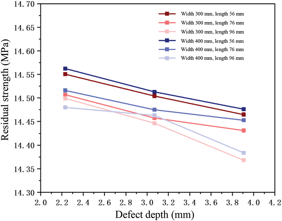
Figure 25: Impact of defect depth on residual strength

Fig. 26 demonstrates failure pressure variation with defect depth across different pipeline wall thicknesses (17.5, 21, 26.2 mm). Corrosion defect depths range from 2% to 40% of wall thickness (2%, 4%, 6%, 8%, 10%, 20%, 30%, 40%), with uniform defect length of Dt and width of 0.05πD.

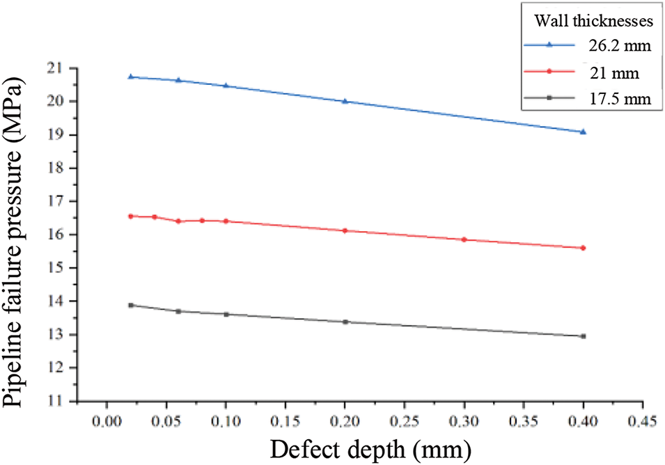
Figure 26: Variation of failure pressure with defect depth in corroded pipelines

Defect depth emerges as a crucial factor affecting pipeline failure pressure. With fixed corrosion defect length, failure pressure decreases rapidly with increasing corrosion depth, showing over 1.7% reduction in failure pressure for each 10% increase in defect depth.

4.3.3 Influence of Wall Thickness on Failure Pressure

Selected scenarios from structural and non-proportional groups compare wall thickness influence on failure pressure. Structural group defects are proportionally sized: length Dt, width 0.05πD, depth 20% of wall thickness across three wall thicknesses. In the non-proportional group, using 21 mm wall thickness as reference, defects measure 146.068 mm length, 159.593 mm width, and 4.2 mm depth.

Fig. 27 illustrates failure pressure variations across different wall thicknesses. Blue points represent proportionally sized defects (structural group), red points represent numerically sized defects (non-proportional group), with three layers corresponding to wall thicknesses of 26.2, 21, and 17.5 mm. Horizontal comparison (green dashed lines) reveals slightly higher failure pressures for proportionally sized defects vs. numerically sized defects at identical wall thickness. Vertical observation indicates significant wall thickness influence on failure pressure regardless of sizing method.

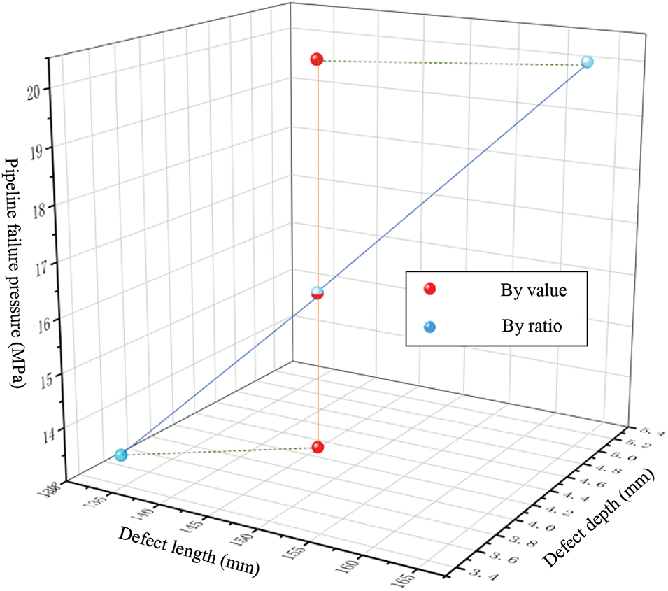
Figure 27: Variation of failure pressure with wall thickness in corroded pipelines

4.3.4 Synergistic Effects and Threshold Analysis

While individual parameter analysis confirms the dominant influence of defect depth on residual strength, our comprehensive investigation reveals previously unexplored synergistic effects between multiple parameters. Specifically, we identified three critical threshold phenomena:

(1) A non-linear interaction between wall thickness and defect depth emerges when defect depth exceeds 30% of wall thickness. At this threshold, the rate of residual strength reduction accelerates from 0.054 MPa per mm to 0.078 MPa per mm, particularly in thicker-walled pipes (26.2 mm). This finding suggests that traditional linear extrapolation methods may underestimate failure risks in severely corroded thick-walled pipelines.

(2) The relationship between defect geometry and failure mechanisms exhibits a distinct transition point. For defects with width-to-length ratios below 0.3, single crack propagation dominates regardless of wall thickness. However, above this threshold, failure patterns bifurcate based on wall thickness: pipes with thickness greater than 21 mm show a higher propensity (73% of cases) for double crack formation, while thinner pipes maintain single crack propagation. This geometry-dependent behavior has significant implications for inspection protocol design and risk assessment strategies.

(3) Analysis of the combined effect of defect depth and circumferential position reveals a previously unidentified critical state. When defect depth reaches 40% of wall thickness in circumferential defects, the traditional advantage of circumferential defects over axial defects in terms of burst pressure resistance diminishes significantly, with the difference reducing from 15% to merely 3%. This finding challenges the conventional understanding of defect orientation effects on pipeline integrity.

These threshold phenomena and their interactions provide new insights for pipeline integrity management, suggesting the need for more nuanced assessment criteria that account for these complex parameter interactions rather than relying solely on individual parameter evaluations.

5  Conclusions

Based on comprehensive numerical simulation and experimental validation of residual strength in corroded pipelines within the Yichang-Qianjiang section, this study has produced several significant findings. Our finite element model demonstrated exceptional reliability, with experimental validation showing deviations consistently within 5% for standard cases, establishing a robust foundation for residual strength prediction. The model remained effective even for complex geometries such as combined axial-circumferential defects, though accuracy decreased slightly to 5.1%–5.4% in these cases.

Analysis of burst evolution processes revealed previously undocumented distinctions in failure patterns between large and small defects. Large defects exhibited stress concentration at circumferential edges with subsequent longitudinal propagation, while small defects concentrated stress centrally before failure. This understanding of failure mechanisms provides crucial insights for defect assessment protocols.

Quantitative parameter analysis yielded specific correlations between defect characteristics and residual strength. Defect depth emerged as the most critical factor, with every 1 mm increase reducing strength by 0.054 MPa, while defect length showed a more moderate influence of 0.0018 MPa reduction per mm. These precise relationships enable more accurate prediction of pipeline deterioration rates. The orientation analysis revealed that circumferential defects exhibited 15% higher burst failure pressure compared to axial defects, though this advantage diminished significantly at depths exceeding 40% wall thickness.

Wall thickness demonstrated substantial influence on failure patterns, with thicker walls (26.2 mm) showing greater tendency toward double crack formation compared to single crack propagation in thinner sections. However, this effect varied with defect geometry, particularly when defect width exceeded 0.075πD combined with lengths exceeding Dt.

These findings have significant implications for pipeline integrity management. The demonstrated relationship between defect depth and strength reduction suggests that depth monitoring should be prioritized in inspection protocols. The distinct behavior of different defect orientations indicates the need for orientation-specific assessment criteria. Furthermore, the interaction between wall thickness and failure patterns highlights the importance of geometry-specific monitoring strategies for pipelines with varying wall thicknesses.

These insights provide a quantitative foundation for developing more targeted inspection strategies and maintenance protocols for corroded pipelines, particularly within the Yichang-Qianjiang section of the Sichuan-East Gas Pipeline. The results enable more accurate risk assessment and better-informed maintenance scheduling, ultimately contributing to enhanced pipeline safety and operational efficiency.

Acknowledgement: None.

Funding Statement: The authors received no specific funding for this study.

Author Contributions: Yaojin Fan: Conceptualization, Methodology; Huaqing Dong: Data curation, Writing—original draft preparation; Zixuan Zong: Investigation; Tingting Long: Methodology; Qianglin Huang: Writing—reviewing and editing; Guoqiang Huang: Writing—reviewing and editing. All authors reviewed the results and approved the final version of the manuscript.

Availability of Data and Materials: Data will be made available on request.

Ethics Approval: None.

Conflicts of Interest: The authors declare no conflicts of interest to report regarding the present study.

References

1. Lu H, Xi D, Xiang Y, Su Z, Cheng YF. Vehicle-canine collaboration for urban pipeline methane leak detection. Nat Cities. 2025. doi:10.1038/s44284-024-00183-w. [Google Scholar] [CrossRef]

2. Di Y, Shuai J, Wang XL, Shi L. Study on methods for classifying oil & gas pipeline incidents. China Saf Sci J. 2013;23(7):109–15 (In Chinese). doi:10.16265/j.cnki.issn1003-3033.2013.07.017. [Google Scholar] [CrossRef]

3. Shuai J, Zhang CE, Chen FL. Comparison study on assessment methods for remaining strength of corroded pipeline. Nat Gas Ind. 2006;26(11):122–5, 184 (In Chinese). [Google Scholar]

4. Li H, Huang K, Zeng Q, Sun C. Residual strength assessment and residual life prediction of corroded pipelines: a decade review. Energies. 2022;15(3):726. doi:10.3390/en15030726. [Google Scholar] [CrossRef]

5. Benjamin AC, Freire JLF, Vieira RD, de Andrade EQ. Burst tests on pipeline containing closely spaced corrosion defects. In: 25th International Conference on Offshore Mechanics and Arctic Engineering; 2006 Jun 4–9; Hamburg, Germany; 2008. p. 103–16. doi:10.1115/OMAE2006-92131. [Google Scholar] [CrossRef]

6. Chen Y, Zhang H, Zhang J, Li X, Zhou J. Failure analysis of high strength pipeline with single and multiple corrosions. Mater Des. 2015;67(32):552–7. doi:10.1016/j.matdes.2014.10.088. [Google Scholar] [CrossRef]

7. Cai J, Jiang X, Lodewijks G, Pei Z, Wu W. Residual ultimate strength of damaged seamless metallic pipelines with combined dent and metal loss. Mar Struct. 2018;61(5):188–201. doi:10.1016/j.marstruc.2018.05.006. [Google Scholar] [CrossRef]

8. Chin KT, Arumugam T, Karuppanan S, Ovinis M. Failure pressure prediction of pipeline with single corrosion defect using artificial neural network. Pipeline Sci Technol. 2020;4(1):10–7. doi:10.28999/2514-541X-2020-4-1-10-17. [Google Scholar] [CrossRef]

9. Zhang H, Tian Z. Failure analysis of corroded high-strength pipeline subject to hydrogen damage based on FEM and GA-BP neural network. Int J Hydrog Energy. 2022;47(7):4741–58. doi:10.1016/j.ijhydene.2021.11.082. [Google Scholar] [CrossRef]

10. Zhou R, Gu X, Luo X. Residual strength prediction of X80 steel pipelines containing group corrosion defects. Ocean Eng. 2023;274(4):114077. doi:10.1016/j.oceaneng.2023.114077. [Google Scholar] [CrossRef]

11. Feng L, Huang D, Chen X, Shi H, Wang S. Residual ultimate strength investigation of offshore pipeline with pitting corrosion. Appl Ocean Res. 2021;117(12):102869. doi:10.1016/j.apor.2021.102869. [Google Scholar] [CrossRef]

12. Lu H, Iseley T, Matthews J, Liao W, Azimi M. An ensemble model based on relevance vector machine and multi-objective salp swarm algorithm for predicting burst pressure of corroded pipelines. J Petrol Sci Eng. 2021;203(1):108585. doi:10.1016/j.petrol.2021.108585. [Google Scholar] [CrossRef]

13. Sun C, Wang Q, Li Y, Li Y, Liu Y. Numerical simulation and analytical prediction of residual strength for elbow pipes with erosion defects. Materials. 2022;15(21):7479. doi:10.3390/ma15217479. [Google Scholar] [PubMed] [CrossRef]

14. Wang Q, Lu H. A novel stacking ensemble learner for predicting residual strength of corroded pipelines. npj Mater Degrad. 2024;8(1):87. doi:10.1038/s41529-024-00508-z. [Google Scholar] [CrossRef]

15. Lu H, Xu ZD, Iseley T, Matthews JC. Novel data-driven framework for predicting residual strength of corroded pipelines. J Pipeline Syst Eng Pract. 2021;12(4):04021045. doi:10.1061/(ASCE)PS.1949-1204.0000587. [Google Scholar] [CrossRef]

16. Chen Z, Li X, Wang W, Li Y, Shi L, Li Y. Residual strength prediction of corroded pipelines using multilayer perceptron and modified feedforward neural network. Reliab Eng Syst Saf. 2023;231(6):108980. doi:10.1016/j.ress.2022.108980. [Google Scholar] [CrossRef]

17. Jiang F, Dong S. Development of an integrated deep learning-based remaining strength assessment model for pipelines with random corrosion defects subjected to internal pressures. Mar Struct. 2024;96(1):103637. doi:10.1016/j.marstruc.2024.103637. [Google Scholar] [CrossRef]

18. Miao X, Zhao H. Novel method for residual strength prediction of defective pipelines based on HTLBO-DELM model. Reliab Eng Syst Saf. 2023;237(4):109369. doi:10.1016/j.ress.2023.109369. [Google Scholar] [CrossRef]

19. Li X, Jia R, Zhang R. A data-driven methodology for predicting residual strength of subsea pipeline with double corrosion defects. Ocean Eng. 2023;279(5500):114530. doi:10.1016/j.oceaneng.2023.114530. [Google Scholar] [CrossRef]

20. Chun PJ, Yamane T, Izumi S, Kameda T. Evaluation of tensile performance of steel members by analysis of corroded steel surface using deep learning. Metals. 2019;9(12):1259. doi:10.3390/met9121259. [Google Scholar] [CrossRef]

21. Nam YJ, Chun PJ, Bae CH, Kim JH, Lim YM. Difference in tensile load-carrying capacity of a corroded water pipeline due to circumferential location. Structures. 2023;58:105357. doi:10.1016/j.istruc.2023.105357. [Google Scholar] [CrossRef]

22. Ansari Sadrabadi S, Dadashi A, Yuan S, Giannella V, Citarella R. Experimental-numerical investigation of a steel pipe repaired with a composite sleeve. Appl Sci. 2022;12(15):7536. doi:10.3390/app12157536. [Google Scholar] [CrossRef]

23. Abtahi SMR, Sadrabadi SA, Rahimi GH, Singh G, Abyar H, Amato D, et al. Experimental and finite element analysis of corroded high-pressure pipeline repaired by laminated composite. Comput Model Eng Sci. 2024;140(2):1783–806. doi:10.32604/cmes.2024.047575. [Google Scholar] [CrossRef]

24. Huang WH, Zheng HL, Li MF. Development history and prospect of oil & gas storage and transportation industry in China. Oil Gas Storage Transp. 2019;38(1):1–11 (In Chinese). [Google Scholar]