Fast Mixture Distribution Optimization for Rain-Flow Matrix of a Steel Arch Bridge by REBMIX Algorithm

1  Introduction

Probabilistic analysis and reliability assessment of civil structures have gained increasing attention in consideration of the inherent uncertainty in loading, environment, and degradation of material properties [1–4]. In the safety assessment for steel bridges, fatigue remains a critical concern for researchers and engineers [5,6]. Probabilistic modeling of rain-flow matrices is crucial within the framework of fatigue reliability assessment using the S-N curve method. Especially, the computational accuracy and efficiency of modeling rain-flow matrices derived from monitoring data play a crucial role in determining the fatigue reliability of steel bridges. Bridges are typically subjected to various types of loadings, such as vehicles, trains, and winds. Each loading type exhibits distinct statistical characteristics [7,8], which contribute to the complexity of the stress responses. As a result, single-mode probability distributions often fail to adequately capture the diversity and complexity of stress spectra derived from rain-flow counting algorithms. This limitation underscores the need for more advanced modeling techniques.

Finite mixture distributions [9] provide a versatile mathematical framework for statistically modeling a wide range of random phenomena. These models have found extensive applications in fields such as cluster analysis, latent class analysis, and the multimodal analysis of observations. By allowing the combination of multiple component distributions, finite mixture models offer a semi-parametric approach that can effectively represent unknown or complex distributional shapes. Finite mixture distributions have been widely used in modeling characteristics of the wind, vehicle loading, and stress spectrum [10–13]. Meanwhile, it is crucial to identify the parameters of finite mixture distributions using well-designed optimal algorithms. These algorithms play a pivotal role in ensuring both computational accuracy and efficiency, which are essential for practical applications. By optimizing the calculation process, they enable the handling of large datasets and complex models with minimal computational resources, which are primary considerations in practical applications.

Over the years, significant research has focused on estimating the parameters of finite mixture distributions. Techniques such as graphical methods, least squares, moment estimation algorithms, and maximum likelihood estimation (MLE) have been widely employed. Among these, the expectation maximization (EM) algorithm [14,15], a notable MLE-based method, has been particularly effective for parameter estimation in distributions like the Weibull distribution [16]. However, a notable limitation of the standard EM algorithm is its tendency to converge rapidly to a local maximum of the likelihood function. This behavior often disregards other promising local optima near the initial guess, potentially resulting in suboptimal solutions. Additionally, the computational efficiency of the EM algorithm can be a concern, particularly for large datasets or complex models, where iterative updates may become computationally expensive.

In recent years, the REBMIX algorithm has emerged as a robust alternative for fitting finite mixture models [17,18]. Implemented in the R package rebmix and refined over time [19–22], REBMIX offers a suite of tools for generating and analyzing random univariate and multivariate finite mixtures. It facilitates the estimation of component numbers, weights, and parameters, as well as bootstrapping and visual representation of mixtures. The REBMIX algorithm addresses finite mixture estimation numerically by decomposing the problem into smaller parameter estimation tasks for basic parametric families. This approach involves iterative optimization of component parameters, mixing weights, and component numbers under specified boundary conditions, such as the maximum allowable number of components or bin counts. The algorithm’s robustness and flexibility make it suitable for initial parameter estimation and model refinement. Finite mixture models have been used in modeling stress ranges [12], with much of the research focusing primarily on modeling accuracy through various algorithms. However, there has been less attention given to using the REBMIX algorithm to model both univariate (stress range) and multivariate (stress range and mean stress) distributions for steel arch bridges. Additionally, the computational efficiency of these models has received limited discussion.

This study explores the application of the REBMIX algorithm in modeling the univariate and multivariate distributions of the rain-flow matrix for a steel arch bridge, employing Akaike’s Information Criterion (AIC) for model evaluation. Four types of finite mixture distributions (normal, lognormal, Weibull, and Gamma) are used to model stress ranges. Additionally, their multivariate counterparts are employed to model the joint distributions of stress range and mean stress. The REBMIX algorithm is applied to estimate the number and weights of components, along with distribution parameters, for each case. Based on these estimates, the probability density function (PDF) and cumulative density function (CDF) are identified, offering a comprehensive approach to mixture parameter estimation.

2  Theoretical Background

2.1 Finite Mixture Model

The use of finite mixture distributions has gained significant traction in recent years for modeling the probability distributions of diverse random phenomena [7]. This method provides a flexible framework to represent complex datasets by combining multiple PDFs into a single composite model. A finite mixture model is essentially a convex combination of two or more component PDFs, each representing a distinct subpopulation or feature within the data. Mathematically, finite mixture distributions for independent scalar or vector observations x can be expressed as a weighted sum of component distributions. This general structure is described as follows:

f(x|c,w,θ)=∑l=1cwlfl(x|θl)(1)

∑l=1cwl=1 and wl≥0(2)

where f(x|c, w, θ) is a predictive mixture density, and fl(x|θl) is a given parametric family of predictive component densities indexed by the scalar or vector parameters θl. The objective of the analysis is an inference about the unknowns which include the number of components or groups, c, the component weights, wl, summing to 1, and the component parameters θl. This approach is particularly valuable for scenarios where the data exhibit heterogeneity or multimodal behavior, as it allows for the decomposition of complex distributions into simpler, interpretable components. Each component captures specific characteristics of the data, while the mixing weights quantify the contribution of each component to the overall distribution. By accommodating multiple underlying patterns, finite mixture models provide a robust tool for tasks such as clustering, classification, and density estimation. Their adaptability and semi-parametric nature have made them an essential method in fields ranging from statistics and machine learning to engineering.

2.2 REBMIX Algorithm

The REBMIX algorithm significantly expands the range of tools available for modeling random univariate and multivariate finite mixtures within the R language and environment for statistical computing [19]. This implementation facilitates tasks such as generating finite mixtures, determining the number of components, estimating component weights and parameters, bootstrapping, and visualizing finite mixture models. Its versatility makes it a valuable resource for statistical analysis and data modeling. The computational process of the REBMIX algorithm involves several key steps, each designed to refine the mixture model iteratively. These steps include preprocessing of observations, global mode detection, clustering of observations, rough component parameter estimation, enhanced component parameter estimation, calculation of first/second moments, and Bayes classification of unassigned observations.

Among the widely used distributions in finite mixture modeling, the REBMIX algorithm supports common forms, such as finite mixtures of normal, lognormal, Weibull, and Gamma distributions. These distributions can be represented mathematically as follows:

f(x|c,w,θ)=∑l=1cwl12πexp⁡{−12(x−μl)2σl2}(3)

f(x|c,w,θ)=∑l=1cwl12πσlxexp⁡{−12(ln⁡(x)−μl)2σl2}(4)

f(x|c,w,θ)=∑l=1cwlγlηl(xηl)γl−1exp⁡{−(xηl)γl}(5)

f(x|c,w,θ)=∑l=1cwl1Γ(γ1)x(xηl)γlexp⁡{−xηl}(6)

where μl and σl represent the mean and standard deviation of the normal mixture components; γl and ηl denote the shape and scale parameters for the Weibull and Gamma mixture components, respectively. Г(γl) is the Gamma function. The parameter estimation of mixture distribution models is deemed a problem of parameter optimization. In this study, the unknown parameters of each distribution are determined by the REBMIX algorithm.

The principles of the algorithm are well described in [22], and its basic process is outlined here. First, the algorithm simultaneously models the number of mixture components, their parameters, and associated weights, providing an initial framework for the mixture distribution. Second, the dataset is divided into a finite number of histogram bins, and the frequency of observations within each bin is calculated, offering a structured representation of the data. Third, the algorithm estimates the parameters and weights of the mixture components, optimizing parameters and assigning observations to their respective component. Finally, each residual observation not initially assigned is distributed among the components based on the Bayes decision rule, ensuring the entire dataset is incorporated into the mixture model. By systematically integrating these steps, the REBMIX algorithm delivers precise and efficient parameter estimation for complex mixture models, making it a reliable tool for modeling heterogeneous data distributions.

In this paper, the specific advantages of the REBMIX algorithm include: (a) its ability to estimate the number of mixture components automatically (only need to set the possible maximum value), which reduces subjectivity in model selection. (b) superior handling of multimodal data distributions in multivariate (stress range and mean stress) distribution of rain-flow matrix. (c) efficiency in parameter estimation, particularly for large datasets, due to its reliance on data preprocessing through clustering, which reduces the computational complexity of parameter initialization and estimation. On the other hand, the key aspects need to explicitly defined: (a) initial parameter settings: The initial parameters, such as the number of components and initial distribution types, are determined based on potential maximum components (10 in this study) and distribution types (including normal distribution, lognormal distribution, Weibull distribution and Gamma distribution in this study); (b) convergence criteria: the modeling normal distribution, lognormal distribution, Weibull distribution and Gamma distribution in this study); (b) convergence criteria: the modeling is defined to have converged when the AIC value stabilizes (see the following Section 2.3).

2.3 Information Criterion

Information criteria play a crucial role in assessing the performance of statistical models, particularly in determining the optimal number of components, the ideal number of bins, and the overall quality of fit for estimated models. By comparing different models, these criteria help identify the most suitable configuration that balances complexity and goodness of fit. In this study, the AIC [23] and the total of positive relative deviations, D, are employed for model evaluation. These metrics serve complementary purposes: AIC provides a measure based on the trade-off between model complexity and data fit, while D assesses the alignment between observed and modeled distributions. The AIC could be mathematically defined as

AIC=−2log⁡L(c,w,Θ)+2M(7)

where M represents the total number of unknown parameters in the model. It is calculated as the product of the number of parameters in a single component distribution and the number of components, c, plus an additional c − 1 to account for the mixing weights. The log-likelihood function, log L (c, w, Θ), represents the likelihood of the observed binned data given the specified model.

The log-likelihood function, which is a measure of how well a model explains the observed data, applies equally to the Parzen window and k-nearest neighbors (k-NN) methods. This ensures that the calculation of the likelihood function remains consistent across different approaches used for non-parametric density estimation. Furthermore, the positive relative deviation for the histogram, a measure of the difference between observed and expected frequencies, can be derived by calculating the sum of the positive deviations for each bin, relative to the expected values.

3  Optimal Distribution Model Selection for Rain-Flow Matrices

3.1 Stress Monitoring Data

In this study, a Structural Health Monitoring (SHM) system was deployed on a steel arch bridge in Hangzhou, China. The bridge spans a total length of 686 m, with a main span of 130 m. To ensure the bridge’s ongoing safety and performance, a network of sensors was installed across key regions to continuously monitor its structural condition. Specifically, 16 measurement zones were selected for sensor placement. Each zone includes three strain measurement points and one temperature compensation point, all strategically positioned at the critical welded joints of the bridge. These joints are at the mid-span and quarter-span sections, areas identified as high-stress zones prone to potential fatigue failure.

The primary focus of this research is on the welded joints that are especially vulnerable to fatigue, particularly those at the rib-to-deck and rib-to-diaphragm connections, which feature cutouts. These areas, located at the bridge’s mid-span, are subjected to considerable cyclic loading, making them prone to the development of fatigue cracks. For this study, the strain data obtained from the sensors on the 7th U-rib in the orthotropic steel deck at the bridge’s mid-span were selected for further analysis. This particular location was chosen due to its critical role in the overall structural behavior of the bridge, as the U-ribs play a key part in distributing the loads across the orthotropic steel deck. The strain measurements from this area, shown in Fig. 1, serve as the primary dataset for evaluating the bridge’s response to various loading conditions and identifying any potential early signs of fatigue or structural degradation.

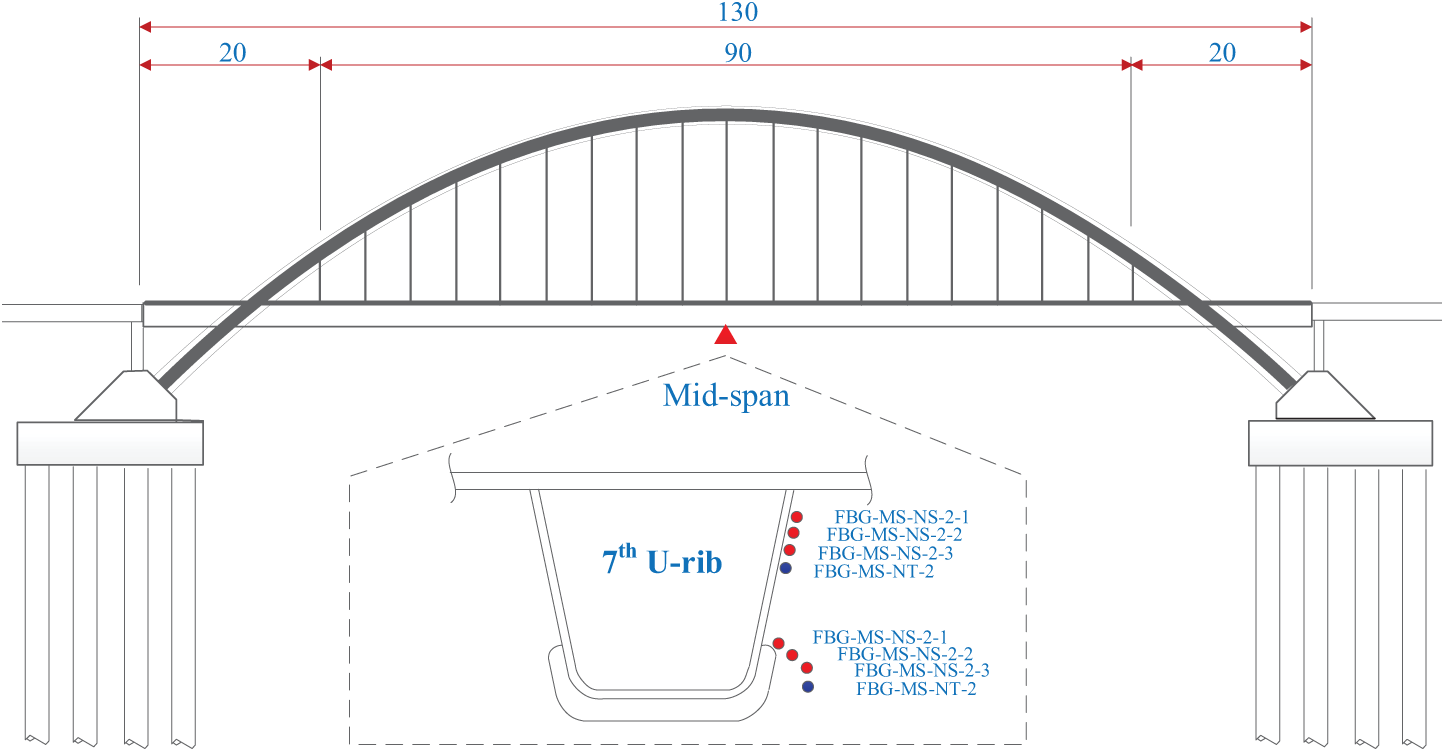
Figure 1: Changyun Bridge and strain sensor deployment at the midspan (unit: m)

3.2 Rain-Flow Matrix

The rain-flow counting algorithm, commonly referred to as the “rain-flow counting method,” is integral to the analysis of fluctuating stress data. Reducing a complex spectrum of varying stresses into a simplified set of stress reversals provides a more practical approach to studying the cyclic nature of loading conditions [24,25]. With advancements in computational technology, the rain-flow counting method has become increasingly accessible and user-friendly, allowing engineers and researchers to efficiently generate rain-flow matrices. These matrices offer valuable insights, such as the stress range (the difference between maximum and minimum stress) and the mean stress (the average of maximum and minimum stress within a cycle). In this study, strain data collected from the 7th U-rib in the orthotropic steel deck at the mid-span of the bridge was used to create a rain-flow matrix. The transformation of this strain data into a rain-flow matrix is shown in Fig. 2. Notably, stress ranges below 3 MPa are excluded from the analysis, as such low-stress ranges have a negligible impact on the fatigue life of the bridge.

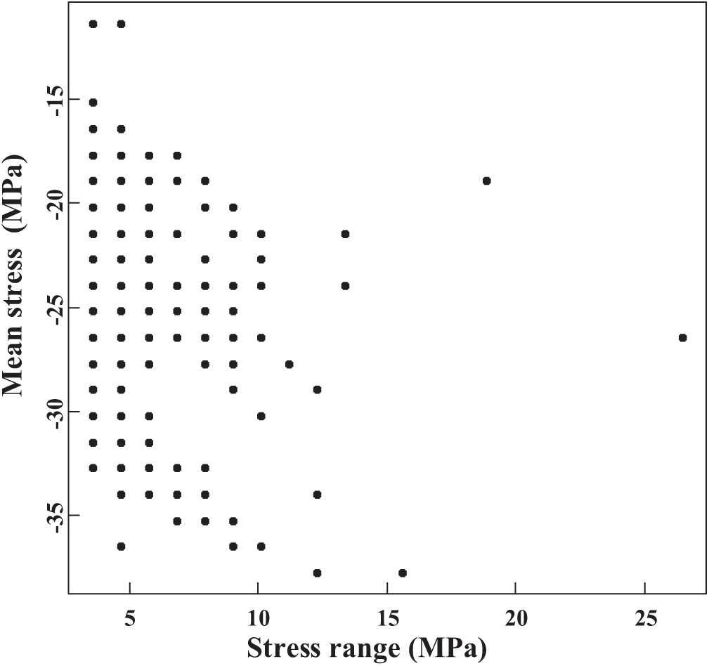
Figure 2: Rain-flow matrix derived from the selected sensor

3.3 Optimal Distribution Model of Stress Range

To assess the probabilistic fatigue life of the steel arch bridge, selecting an appropriate distribution for the stress spectrum, following the rain-flow counting algorithm, is crucial. Typically, fatigue life evaluations focus primarily on the stress range, often overlooking the influence of mean stress for simplicity. However, in this study, the first step is to model the stress range using univariate analysis to determine the most suitable distribution model. The candidate models considered include finite mixed normal distributions, finite mixed lognormal distributions, finite mixed Weibull distributions, and finite mixed Gamma distributions.

For the preprocessing of the histogram, the maximum number of components is limited to 10, with the analysis conducted using the R software package rebmix. This software is employed to fit the stress range data to the various distribution models. The effectiveness and suitability of each distribution model are assessed using the AIC, which provides a quantitative measure for comparing the relative goodness of fit of each model. The model with the lowest AIC value is selected as the optimal distribution, offering the best balance between model complexity and explanatory power.

For the normal distribution, the optimal number of components is determined to be 4, with an AIC value of 1700. It indicates that a mixture of four normal distributions provides the best fit for the data according to the AIC. Fig. 3 illustrates the PDF and CDF of the mixed normal distributions, visually demonstrating how the stress ranges are distributed across the various components. The estimated mean values for each component are 3.32, 3.92, 4.54, and 8, with standard deviations of 0.176, 0.258, 0.316, and 2.73, respectively. The standard deviation for the fourth component is relatively high due to the larger range. This increased variability is likely caused by the extreme or outlier stress values, which contribute to the broader range of stresses observed in the distribution. Such components may represent more significant, less frequent stress events that occur under specific loading conditions. Identifying this component is crucial for accurately modeling fatigue behavior, as it helps predict the impact of these extreme stress cycles on the bridge’s overall fatigue life.

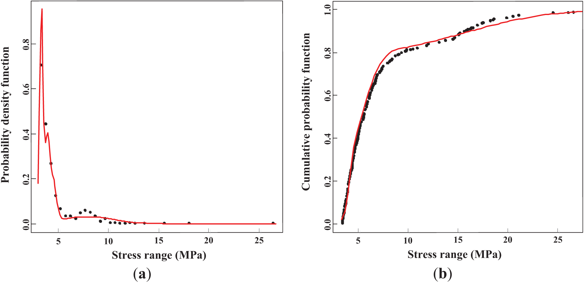
Figure 3: Estimated mixed normal distributions: (a) PDF; (b) CDF

For the lognormal distribution, the optimal number of components is determined to be 4 with an AIC value of 1656, which is lower than the AIC value for the normal distribution, indicating a better fit for the data. The estimated mean value μ of each component is 1.23, 1.46, 2.03, and 2.65 with the standard deviations σ of 0.0735, 0.102, 0.173, and 0.299, respectively. As shown in Fig. 4, it can be easily found that the performance of the lognormal distribution is better than the normal distribution just as the lower AIC value shows. The improved performance of the lognormal distribution is especially apparent when comparing the fit of the two distributions. The lognormal distribution’s ability to better capture the skewed nature of the stress range data makes it a more appropriate model for this particular case, where stress values may not be symmetrically distributed, and a positive skew is often observed.

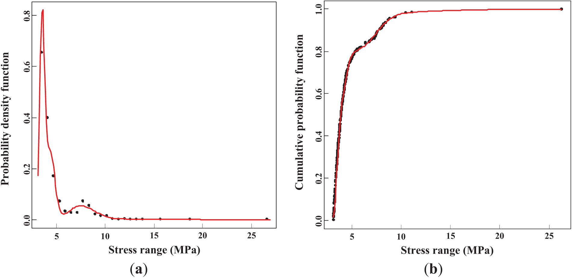
Figure 4: Estimated mixed lognormal distributions: (a) PDF; (b) CDF

Similarly, the number of components and their corresponding parameters for the mixed Weibull distributions are estimated using the REBMIX algorithm. The optimal number of components for the Weibull distribution is determined to be 3, with an AIC value of 1789. This suggests that a mixture of three Weibull distributions provides the best fit for the data in this case. The estimated parameters characterize the Weibull distribution’s ability to model different aspects of the stress range data, with the shape parameter influencing the distribution’s form and the scale parameter affecting the overall spread of values. As shown in Fig. 5, the PDF and CDF of the mixed Weibull distributions provide a visual representation of how well this model fits the stress range data. The shape parameters indicate that the components in the mixture vary significantly in terms of their behavior, with some components modeling more gradual stress range distributions and others capturing more extreme stress events.

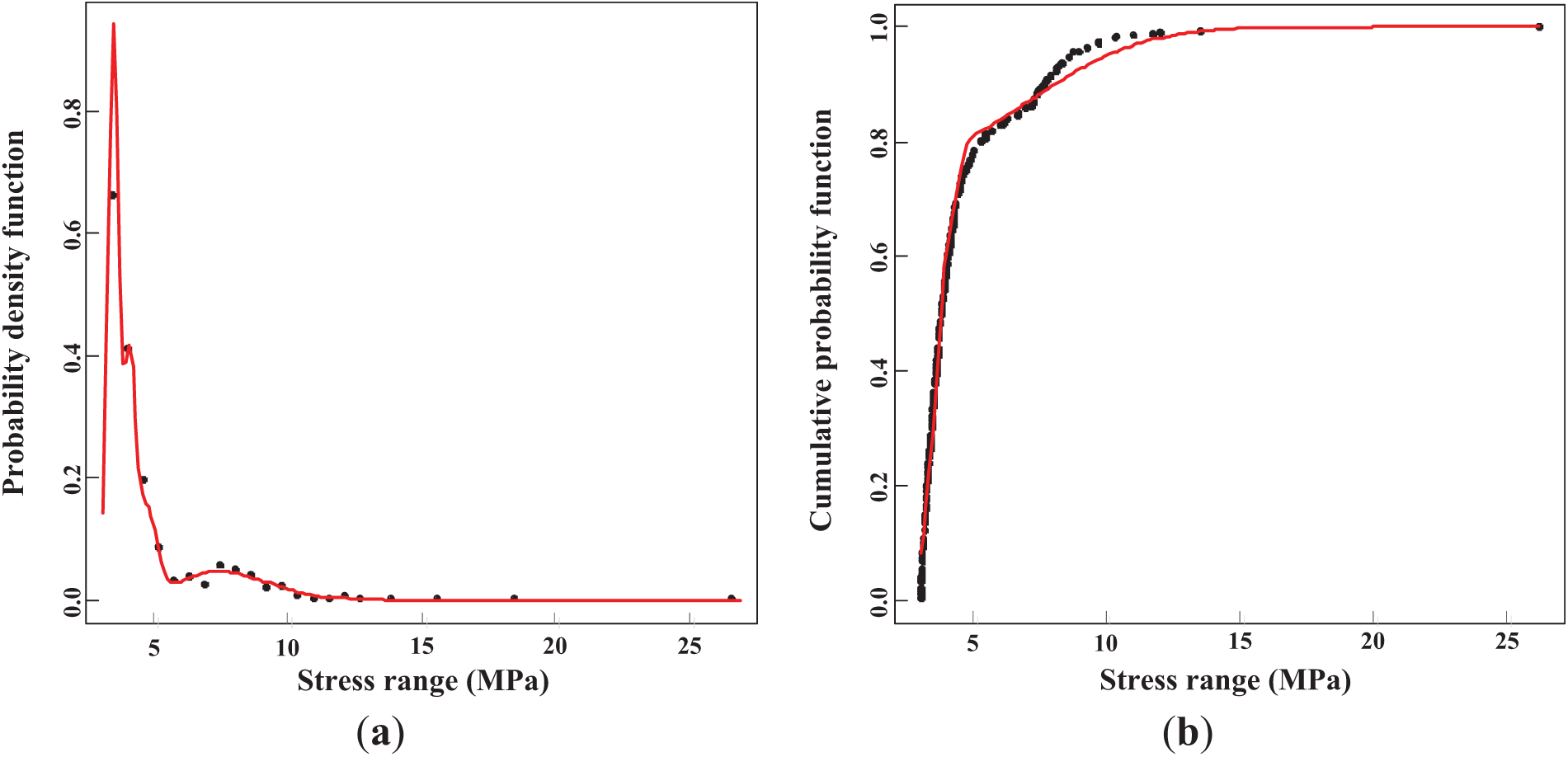
Figure 5: Estimated mixed Weibull distributions: (a) PDF; (b) CDF

The number of components and corresponding parameters for the mixed Weibull distribution were estimated. The optimal number of components for the Weibull distribution is 3, with an AIC value of 1789. The estimated shape parameters (γ) for each component are 3.63, 4.45, and 8.62, with scale parameters (η) of 10.7, 13.3, and 2.66, respectively. Fig. 5 displays both the PDF and CDF of the mixed Weibull distributions. The optimal number of components for the Gamma distribution is 4, with an AIC value of 1699. Fig. 6 shows the PDF and CDF of the mixed Gamma distributions. In this case, the Gamma distribution offers a superior fit to the data compared to the commonly used Weibull distribution. It models stress ranges with greater precision, effectively capturing frequent smaller stress events and rarer, more extreme stress cycles.

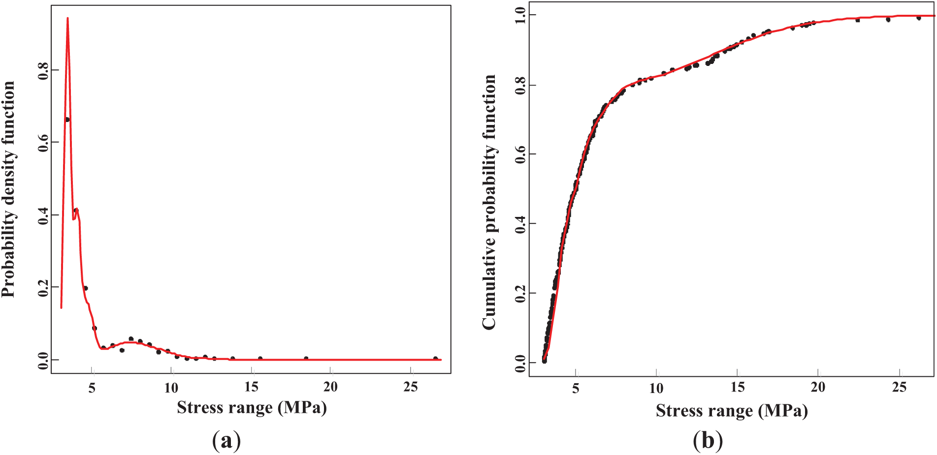
Figure 6: Estimated mixed Gamma distributions: (a) PDF; (b) CDF

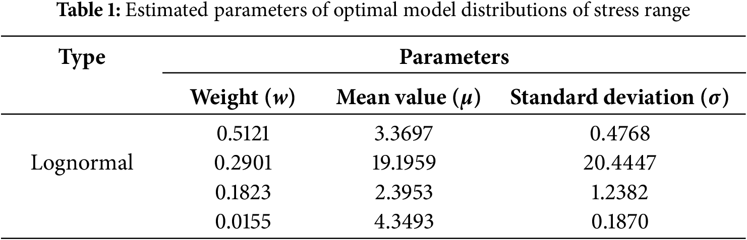
In summary, the optimal distribution model for the stress range is the 4-component mixed lognormal distribution, which provides the best fit with an AIC value of 1656. This model outperforms the other candidate distributions, such as normal, Weibull, and Gamma, based on its lower AIC value. The lognormal distribution’s ability to capture the skewness in the data and its flexibility in modeling stress variations make it particularly suitable for this analysis. The estimated parameters for the optimal mixed lognormal model, including the mean and standard deviation for each component, are summarized in Table 1. These parameters provide detailed insights into the distribution of stress ranges, which are critical for accurately assessing the probabilistic fatigue life of the steel arch bridge.

3.4 Optimal Distribution Model of Rain-Flow Matrix

The impact of the mean value on fatigue life is considered in the Goodman fatigue model [26,27]. According to this model, the same stress range with different mean stress values can result in varying fatigue life outcomes [28–31]. Typically, higher mean stress leads to a shorter fatigue life, as the structure is already under a higher baseline stress, making it more susceptible to failure under cyclic loading. To accurately account for this influence, it is essential to use an optimal distribution model that incorporates both the stress range and the mean stress when the effect of the mean stress cannot be ignored.

The distribution model of the rain-flow matrix is extended to include both the stress range and mean stress, providing a more comprehensive understanding of the bridge’s fatigue behavior. It is important to note that the mean stress is assumed to follow a normal distribution. This assumption arises from the fact that the mean stress typically has a negative value, which is commonly observed in cyclic loading scenarios, as shown in Fig. 7. The REBMIX algorithm offers powerful functions for generating both univariate and multivariate finite mixtures, as well as estimating the number of components, their weights, and the parameters associated with each component.

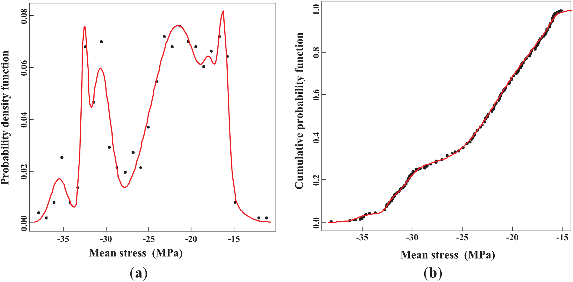
Figure 7: Mixed normal distributions of mean value: (a) PDF; (b) CDF

This section focuses on the multivariate modeling of the rain-flow matrix to identify the optimal distribution model. Several candidate models are considered, including finite mixed normal-normal distributions, finite mixed lognormal-normal distributions, finite mixed Weibull-normal distributions, and finite mixed Gamma-normal distributions. To preprocess the histogram data, the maximum number of components is set to 10, allowing for a more flexible and detailed representation of the distribution while maintaining computational feasibility. Each candidate distribution model is evaluated based on its performance, quantified using the AIC value. As with univariate modeling, the AIC is used to identify the distribution that best represents the data while avoiding overfitting, considering the complex interactions between stress range and mean stress.

For the mixed normal-normal distribution, the optimal number of components is determined to be 5, with an AIC value of 5313. This indicates that the five-component mixture provides the best fit to the data among the considered models. Fig. 8 presents both the PDF and CDF of the mixed normal-normal distributions. The PDF in Fig. 8 illustrates the relative likelihood of different stress values occurring, with each component contributing to the overall distribution. The CDF provides a cumulative perspective, showing the probability that the stress range will fall below a specific value. The five-component mixed normal-normal distribution offers a detailed and flexible representation of the stress range data, capturing the complexity of the observed loading patterns.

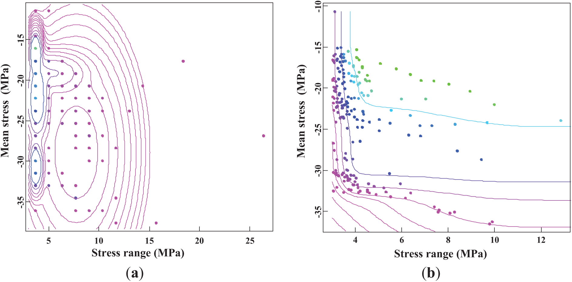
Figure 8: Estimated mixed normal-normal distributions: (a) PDF; (b) CDF

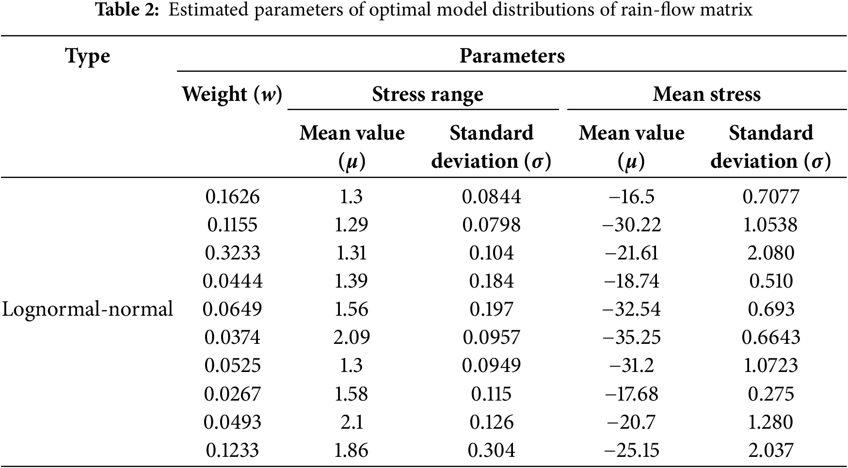
Fig. 9 demonstrates that a 10-component mixture provides the best fit to the data when considering the lognormal-normal distribution. To validate the robustness of this result, the maximum number of components is set to 20. In this case, the optimal number of components remained at 10, indicating that increasing the maximum number of components did not improve the model’s fit. This consistency suggests that a 10-component mixture is appropriate and efficient. The estimated parameters of optimal model distributions are shown in Table 2.

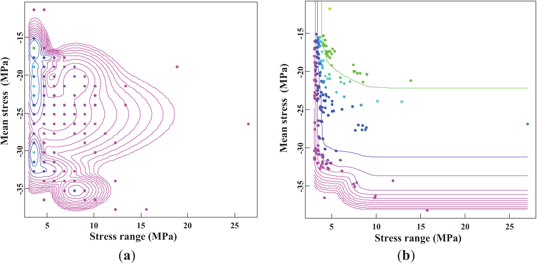
Figure 9: Estimated mixed lognormal-normal distributions: (a) PDF; (b) CDF

When comparing the lognormal-normal distribution to the normal-normal distribution, the former exhibits superior performance, as reflected by its lower AIC value. Despite having more components, the lognormal-normal distribution provides a more accurate representation of the stress data. It suggests that the lognormal distribution is better suited to capturing the skewed nature of the data, a characteristic commonly observed in real-world fatigue scenarios, where stress values are not symmetrically distributed.

The number of components and corresponding parameters for the mixed Weibull-normal distributions are estimated using the REBMIX algorithm. The optimal number of components is 8, with an AIC value of 5384, indicating that an eight-component mixture is the best fit for the data within the defined framework. Both the shape and scale parameters for each component are precisely determined. Fig. 10 illustrates the probability density function (PDF) and cumulative density function (CDF) of the mixed Weibull-normal distributions. Similarly, the performance of the Gamma-normal distribution is evaluated in this study. The optimal number of components for the Gamma-normal distribution is 6, with an AIC value of 5108. Fig. 11 presents the PDF and CDF of the mixed Gamma-normal distributions, providing a comprehensive view of the distribution’s fit.

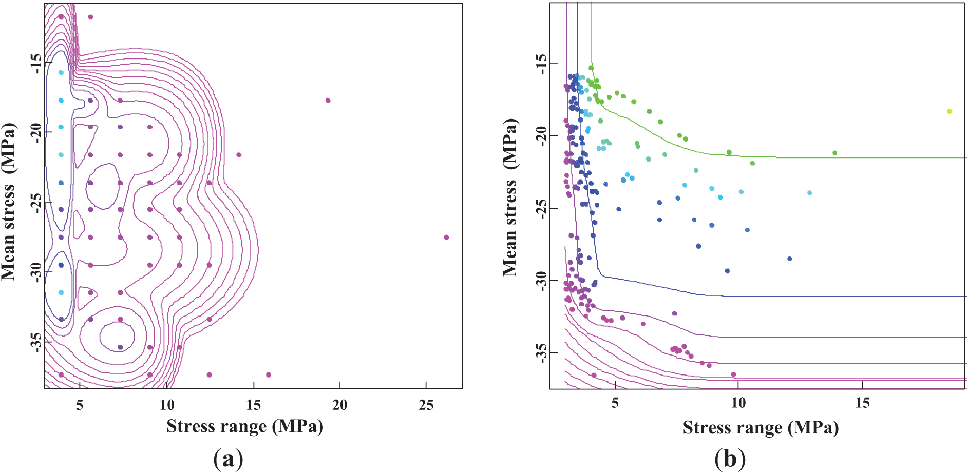
Figure 10: Estimated mixed Weibull-normal distributions: (a) PDF; (b) CDF

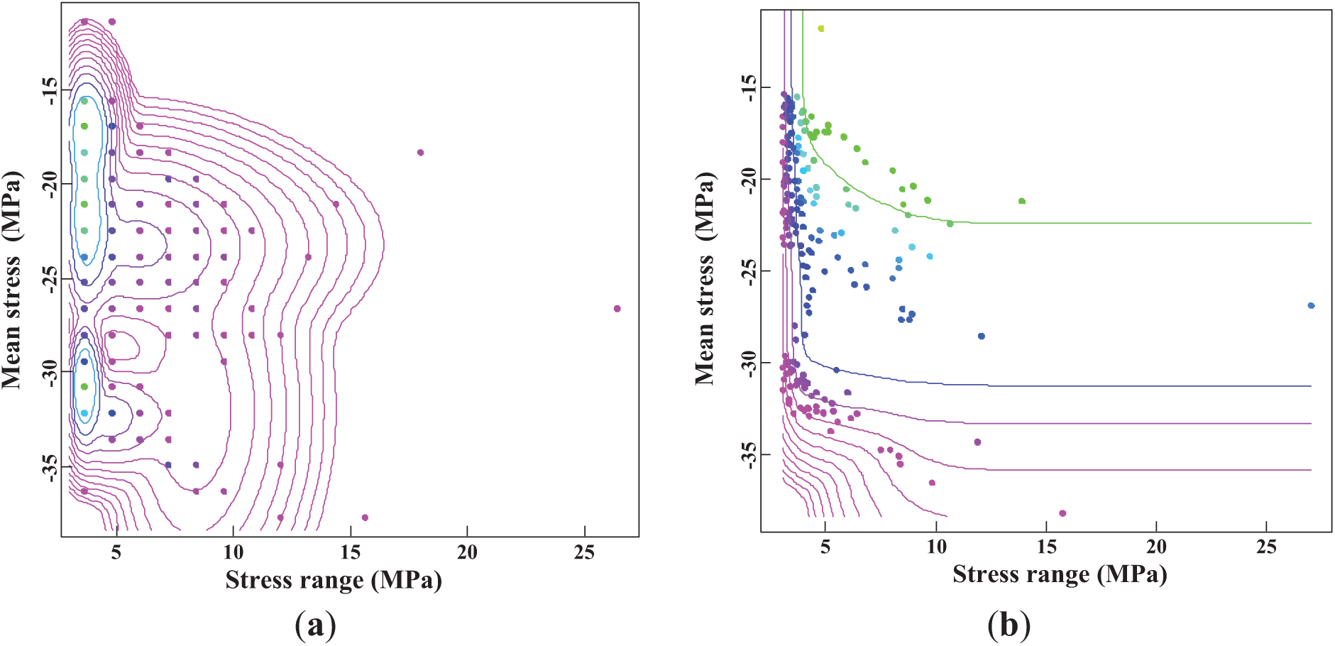
Figure 11: Estimated mixed Gamma-normal distributions: (a) PDF; (b) CDF

It is significant to highlight that the entire estimation process for both univariate (stress range) and multivariate (stress range and mean stress) distributions of the rain-flow matrix can be efficiently carried out using the REBMIX algorithm. Moreover, a comparative analysis of its performance against other commonly used algorithms is provided. This analysis considers metrics such as computation time and estimation accuracy. Compared to the EM algorithm and genetic algorithm (GA), the REBMIX algorithm completes parameter estimation in just 10 s, as shown in Fig. 12. This computational advantage is particularly valuable when handling large datasets or complex models. The REBMIX algorithm’s ability to quickly and accurately estimate parameters enhances its practical utility for more efficient and timely fatigue life assessments of civil structures, such as the steel arch bridge in this study.

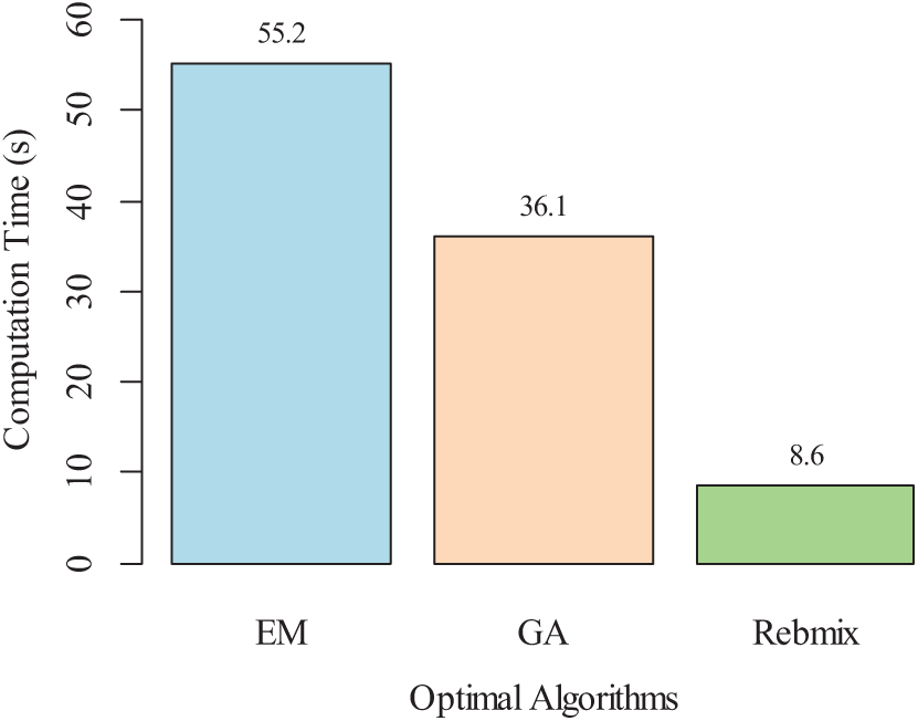
Figure 12: Comparative analysis of algorithm performance in computation times

4  Concluding Remarks

This study evaluates the performance of the REBMIX algorithm in modeling the univariate (stress range) and multivariate (stress range and mean stress) distributions of the rain-flow matrix for a steel arch bridge, using AIC as a performance metric. Four types of finite mixture distributions—normal, lognormal, Weibull, and Gamma—are employed to model the stress range. Additionally, mixed distributions, including normal-normal, lognormal-normal, Weibull-normal, and Gamma-normal, are used to model the joint distribution of stress range and mean stress. The REBMIX algorithm estimates the number of components, component weights, and component parameters for each candidate finite mixture distribution. The results reveal the following:

1.    The REBMIX algorithm-based mixture parameter estimation approach has a favorable capability in estimating the parameters of mixture distribution models of the rain-flow matrix of steel arch bridge;

2.    The mixed lognormal distributions and lognormal-normal distributions are the optimal distributions of the rain-flow matrix in this study;

3.    The REBMIX algorithm is time-effective in computer calculation procedures when considering the computational efficiency of parameter estimation.

Furthermore, sensitivity analyses will be conducted in future work to gain a deeper understanding of how different model selections impact the variability in fatigue life estimates. This will involve systematically testing various models and assessing their influence on the predictions of fatigue life under different conditions.

Acknowledgement: Specially thank the professional technical support to the study by the members of our research group at Shaoxing University, Zhejiang University, and Xi’an Jiaotong University.

Funding Statement: The work described in this paper was jointly supported by the Fundamental Research Funds for the Central Universities (Grant No. xzy012023075), the Zhejiang Engineering Research Center of Intelligent Urban Infrastructure (Grant No. IUI2023-YB-12).

Author Contributions: The authors confirm their contribution to the paper as follows: study conception and design: Yuliang He, Youhua Su; data collection: Weihong Lou, Da Hang, Youhua Su; analysis and interpretation of results: Yuliang He, Weihong Lou, Da Hang, Youhua Su; draft manuscript preparation: Yuliang He, Weihong Lou, Da Hang, Youhua Su. All authors reviewed the results and approved the final version of the manuscript.

Availability of Data and Materials: The authors confirm that the data supporting the findings of this study are available within the article.

Ethics Approval: Not applicable.

Conflicts of Interest: The authors declare no conflicts of interest to report regarding the present study.

References

1. Chen RP, Jiang P, Ye XW, Bian XC. Probabilistic analytical model for settlement risk assessment of high-speed railway subgrade. J Perform Constr Facil. 2016;30(3):04015047. doi:10.1061/(ASCE)CF.1943-5509.0000789. [Google Scholar] [CrossRef]

2. Kordestani H, Xiang YQ, Ye XW, Jia YK. Application of the random decrement technique in damage detection under moving load. Appl Sci. 2018;8(5):753. doi:10.3390/app8050753. [Google Scholar] [CrossRef]

3. Ding Y, Ye XW, Su YH, Zheng XL. A framework of cable wire failure mode deduction based on Bayesian network. Structures. 2023;57(1):104996. doi:10.1016/j.istruc.2023.104996. [Google Scholar] [CrossRef]

4. Su YH, Ye XW, Ding Y, Chen B. Data-driven fatigue failure probability updating of OSD by Bayesian backward propagation. Struct Control Health Monit. 2024;2024(1):2353457. doi:10.1155/2024/2353457. [Google Scholar] [CrossRef]

5. Maiorana E, Aloisio A, Tasse V, Briseghella B. Prediction of fatigue life of a bolted joint in a railway steel arch bridge using multiaxial fatigue criteria. Eng Fail Anal. 2024;166:108908. doi:10.1016/j.engfailanal.2024.108908. [Google Scholar] [CrossRef]

6. Yu M, Xie X. Ultra-low cycle fatigue life prediction of stainless steel based on transfer learning guided artificial neural network. Eng Appl Artif Intel. 2024;136:109054. doi:10.1016/j.engappai.2024.109054. [Google Scholar] [CrossRef]

7. Ni YQ, Ye XW, Ko JM. Monitoring-based fatigue reliability assessment of steel bridges: analytical model and application. J Struct Eng. 2010;136(12):1563–73. doi:10.1061/(ASCE)ST.1943-541X.0000250. [Google Scholar] [CrossRef]

8. Ni YQ, Ye XW, Ko JM. Modeling of stress spectrum using long-term monitoring data and finite mixture distributions. J Eng Mech. 2012;138(2):175–83. doi:10.1061/(ASCE)EM.1943-7889.0000313. [Google Scholar] [CrossRef]

9. McLachlan GJ, Peel D. Finite mixture models. Hoboken, NJ, USA: John Wiley & Sons; 2000. [Google Scholar]

10. Ye XW, Su YH, Xi PS, Chen B, Han JP. Statistical analysis and probabilistic modeling of WIM monitoring data of an instrumented arch bridge. Smart Struct Syst. 2016;17(6):1087–105. doi:10.12989/sss.2016.17.6.1087. [Google Scholar] [CrossRef]

11. Ye XW, Xi PS, Su YH. Analysis of non-stationary wind characteristics at an arch bridge using structural health monitoring data. J Civ Struct Health. 2017;7:573–87. doi:10.1007/s13349-017-0244-5. [Google Scholar] [CrossRef]

12. Su YH, Ye XW, Ding Y. ESS-based probabilistic fatigue life assessment of steel bridges: methodology, numerical simulation, and application. Eng Struct. 2022;253:113802. doi:10.1016/j.engstruct.2021.113802. [Google Scholar] [CrossRef]

13. Ding Y, Ye XW, Guo Y. Copula-based JPDF of wind speed, wind direction, wind angle, and temperature with SHM data. Probabilistic Eng Mech. 2023;73:103483. doi:10.1016/j.probengmech.2023.103483. [Google Scholar] [CrossRef]

14. Dempster A, Laird N, Rubin D. Maximum likelihood from incomplete data via the EM algorithm. J R Stat Soc: Ser B (Methodol). 1977;39(1):1–38. doi:10.1111/j.2517-6161.1977.tb01600.x. [Google Scholar] [CrossRef]

15. Moon TK. The expectation-maximization algorithm. IEEE Signal Proc Mag. 1997;13(6):47–60. doi:10.1109/79.543975. [Google Scholar] [CrossRef]

16. Panteleeva OV, González EG, Huerta HV, Alva JAV. Identifiability and comparison of estimation methods on Weibull mixture models. Commun Stat-Simul C. 2015;44(6):1879–900. doi:10.1080/03610918.2013.839031. [Google Scholar] [CrossRef]

17. Nagode M, Fajdiga M. An improved algorithm for parameter estimation suitable for mixed Weibull distributions. Int J Fatigue. 2000;22(1):75–80. doi:10.1016/S0142-1123(99)00112-7. [Google Scholar] [CrossRef]

18. Nagode M, Fajdiga M. An alternative perspective on the mixture estimation problem. Reliab Eng Syst Safe. 2006;91(4):388–97. doi:10.1016/j.ress.2005.02.005. [Google Scholar] [CrossRef]

19. Nagode M. Finite mixture modeling via REBMIX. J Algorithms Optim. 2015;3(2):14–28. doi:10.5963/JAO0302001. [Google Scholar] [CrossRef]

20. Nagode M, Oman S, Klemenc J, Panić B. Gumbel mixture modeling for multiple failure data. Reliab Eng Syst Safe. 2023;230:108946. doi:10.1016/j.ress.2022.108946. [Google Scholar] [CrossRef]

21. Nagode M, Panić B, Klemenc J, Oman S. Fault detection and classification with the rebmix R package. Comput Ind Eng. 2023;185:109628. doi:10.1016/j.cie.2023.109628. [Google Scholar] [CrossRef]

22. Nagode M. rebmix: finite mixture modeling, clustering & classification [Internet]. [cited 2025 Jan 1]. Available from: http://CRAN.R-project.org/package=rebmix. [Google Scholar]

23. Akaike H. A new look at the statistical model identification. IEEE T Automat Contr. 1974;19(6):716–23. doi:10.1109/TAC.1974.1100705. [Google Scholar] [CrossRef]

24. Matsuishi M, Endo T. Fatigue of metals subjected to varying stress. Jpn Soc Mech Eng. 1968;68(2):37–40. [Google Scholar]

25. Downing SD, Socie DF. Simple rain-flow counting algorithms. Int J Fatigue. 1982;4(1):31–40. doi:10.1016/0142-1123(82)90018-4. [Google Scholar] [CrossRef]

26. Goodman J. Mechanics applied to engineering. London, UK: Longman, Green & Company; 1899. [Google Scholar]

27. Nicholas T, Zuiker JR. On the use of the goodman diagram for high cycle fatigue design. Int J Fract. 1996;80(2):219–35. doi:10.1007/BF00012670. [Google Scholar] [CrossRef]

28. Dowling NE, Calhoun CA, Arcari A. Mean stress effects in stress-life fatigue and the Walker equation. Fatigue Fract Eng M. 2009;32(3):163–79. doi:10.1111/j.1460-2695.2008.01322.x. [Google Scholar] [CrossRef]

29. Zhang Z, He Z, Yang B, Wang Y, Xiao S, Hou M, et al. An improved Goodman-Smith fatigue limit diagram for railway vehicle base metals and welded structures. Int J Fatigue. 2024;182:108160. doi:10.1016/j.ijfatigue.2024.108160. [Google Scholar] [CrossRef]

30. Wu Q, Zhao Y, Liu X. Fatigue life prediction of metal materials under random loads based on load spectrum extrapolation. Int J Fatigue. 2024;187:108473. doi:10.1016/j.ijfatigue.2024.108473. [Google Scholar] [CrossRef]

31. Fernández-Canteli A, Castillo E, Díaz-Salamanca D, Muñiz-Calvente M, Seitl S. Advances in low cycle fatigue probabilistic modeling. Theor Appl Fract Mech. 2024;133:104611. doi:10.1016/j.tafmec.2024.104611. [Google Scholar] [CrossRef]