Acceleration Response Reconstruction for Structural Health Monitoring Based on Fully Convolutional Networks

1  Introduction

The structural health monitoring (SHM) system utilizes communication and sensing devices to automatically collect real-time response signals from structures. This serves as the foundational information for real-time warnings and safety assessments of structures, providing a basis for maintenance and management decisions [1]. Constrained budgets generally necessitate strategically placing a limited number of sensors at key locations, making the monitoring data from each sensor highly important [2,3]. However, during long-term monitoring, technical issues such as cable connection failures, signal transmission interference, sensor malfunctions, or periodic maintenance may result in the loss of measurement data from one or more sensors. While replacing faulty sensors is possible, missing data during maintenance must be reconstructed using appropriate technologies. The loss of one or more signal channels can significantly undermine the effectiveness of structural monitoring and result in the omission of critical local details of the bridge. Consequently, reconstructing the missing data is essential for achieving accurate assessments of structural health conditions [4].

Structural response reconstruction methods can be broadly categorized into two types: finite element-based methods and data-driven methods. In finite element-based methods, Zhang and Wu [5] utilized a moving window Kalman filter (MWKF) with unknown measurement noise covariance (MNC) to integrate both strain and displacement measurements, reconstructing the structural response at unmeasured locations. Xu et al. [6] conducted a numerical study on the selection of sensor types, quantities, and locations using an updated finite element model and reconstructed the response of an actual bridge using measured responses from multiple sensor types. Zhang et al. [7] proposed an adaptive modal selection method based on Kalman filtering, achieving accurate response reconstruction through the application of modal signal-to-noise ratio (MSNR). Zhu et al. [8] introduced a dynamic response reconstruction method based on multi-rate Kalman filtering (MRKF). However, due to inevitable geometric uncertainties, material uncertainties, and variations in environmental and operational conditions, the inherent nature of finite element-based methods limits their applicability in recovering monitoring data for specific locations on complex long-span bridges under constantly changing environments and operational conditions [9]. Given the significant challenges in constructing a finite element model that can precisely reflect the actual behavior of a structure in service, it may even be impossible to achieve [10]. Therefore, these methods are challenging to apply to actual bridges.

The Data-driven approaches are non-finite element methods that bypass the complexity of model construction and directly utilizes measured time-series data for analysis. Among traditional data-driven methods, response reconstruction methods based on compressed sensing (CS) have proven effective in recovering short-term missing data [11]. For random discrete data loss, Bao et al. [12] utilized a machine learning approach based on compressed sensing for reconstruction, proposing an improved complex multi-task Bayesian algorithm for the compression and reconstruction of high-sampling-rate SHM data. Wan et al. [13] introduced an improved Bayesian multi-task learning method that uses measurement data from the same sensor to recover short-term continuous missing acceleration data. However, these approaches do not fully harness the inherent spatial and temporal interdependencies within the monitoring data, and can only use measurements from a single sensor to recover the lost data of that specific sensor [9]. Compared to discrete single-point data loss, continuous data loss is much more difficult to reconstruct. Therefore, these methods fail to achieve high-precision reconstruction of long-term responses.

Due to its outstanding performance in extracting hidden features from data, deep learning has attracted significant attention across various research fields [14]. Current advancements in deep learning focus primarily on using features such as crack images and vibration responses as inputs to networks for structural visual inspection and damage detection [15–17]. Given the similarity between structural response reconstruction and one-dimensional image restoration, deep learning shows significant potential for improving response reconstruction in SHM [18]. In the field of response reconstruction, researchers have proposed techniques such as densely connected convolutional networks, self-attention enhanced generative adversarial networks, and segmented generative adversarial networks [9,19,20]. These methods train generators to extract features from pre-failure measurement data sets and use structural responses from the remaining normal sensors to reconstruct the lost or corrupted signals. Jeong et al. [21] considered the spatiotemporal correlation between sensor data and proposed a sensor data reconstruction method based on recurrent neural networks (RNN). Wang et al. [22] proposed a deep learning-based framework that utilizes temperature monitoring data to reconstruct long-term missing beam-end displacement data in the SHM system of suspension bridges. Oh et al. [23] proposed a method that employs convolutional neural networks (CNN) to reconstruct missing structural responses, validating its applicability with strain monitoring data from an elevated bridge. However, due to the complex non-stationary and nonlinear characteristics of acceleration monitoring data from long-span bridges, traditional data-driven models exhibit decreased reconstruction performance. To address this challenge, the fully convolutional networks (FCN) represent a cutting-edge technique in deep learning for time series prediction. FCN is an evolution and extension of CNN. In addition to the general characteristics of CNN, FCN features full convolution, upsampling, and skip connections, significantly improving its ability to learn complex features. FCN is capable of predicting semantic labels for each pixel, making it particularly suitable for pixel-level tasks, and widely used in fields such as object detection and image recognition [24–26]. By leveraging the FCN model’s ability to extract detailed patterns in time series data and considering the spatiotemporal correlations within a complex sensor network on a bridge, it is possible to reconstruct missing acceleration responses for bridge monitoring.

Therefore, this paper introduces a method for response reconstruction utilizing FCN. By taking into account the complex non-stationary and nonlinear characteristics of the acceleration responses of long-span bridges, an end-to-end FCN model is constructed to reconstruct the acceleration responses. Since the input includes both temporal and spatial information, both types of correlations can be considered simultaneously. By using the reconstruction of acceleration data from an experimental arch rib as an example, a comparative analysis is conducted on the reconstruction capabilities of various neural network models. The method is validated through the reconstruction of measured acceleration responses of a long-span bridge, with a comprehensive parameter analysis discussing the impact of sensor spatial position and quantity on reconstruction performance, thereby demonstrating the effectiveness of the proposed method.

The subsequent sections of this paper are outlined below. The detailed configuration of FCN is introduced in Section 2, including the network architecture and related parameters. It also covers data preprocessing and evaluation metrics. In Section 3, the acceleration response of an experimental arch rib structure is collected, and a comparative study on the reconstruction performance of missing data using different network models is conducted. Section 4 presents the application of the proposed method to reconstruct the health monitoring response of a long-span bridge. Parameter analysis is performed in Section 5 to assess the effectiveness of the introduced reconstruction methods. Section 6 provides a conclusion of the paper.

2  Methodology for Acceleration Response Reconstruction

2.1 Response Reconstruction Framework

In bridge operations, random factors such as noise and environmental effects pose significant challenges by causing continuous data loss. This requires investigating the long-term spatiotemporal correlations to mitigate these issues. The U-net model serves as the foundational network architecture in this paper, driving the development of a highly effective FCN model. Key features of the model include skip connections that preserve low-level details and improve gradient flow, as well as dropout techniques to prevent overfitting and enhance feature extraction. The efficacy of the reconstruction results is evaluated by comparing the reconstructed and actual responses in the time domain and frequency domain. The results demonstrate that the designed FCN model effectively reconstructs missing acceleration responses in structural systems. Through the creation of a sophisticated nonlinear mapping between the input and output responses, the FCN model can accurately predict the missing data points, highlighting its potential as a powerful tool for acceleration response reconstruction in complex systems.

Fig. 1 provides an overview of the proposed method, which includes the following steps: (i) Utilizing a sliding window to prepare training samples; (ii) establishing and training the FCN model; (iii) evaluating the reconstruction results in the time domain and frequency domain. (iv) perform error analysis and parameter analysis.

Figure 1: Overview of the introduced method: (1) Data preparation, (2) Model training, (3) Data recovery, (4) Result evaluation

2.2 Dataset Preparation

A sufficient number of training samples is essential for effectively learning the spatiotemporal correlations between sensors. The actual bridge response data is typically a long time series, which is segmented to ensure an adequate number of samples from the raw response data. A sliding window is used to segment the original data as follows:

M=(W−R)/Q+1(1)

where M is the number of samples; W represents the length of the initial response; R is the sliding window length; Q is the window stride.

The data samples were partitioned randomly into training and validation sets with an 8:2 ratio. To accelerate network convergence and improve reconstruction accuracy, the sample data was normalized. The pre-processed data undergoes scaling to fit within a −1 to 1 range by:

Aijk′=Aijkmax(|A|),i∈[1,R],j∈[1,C],k∈[1,M](2)

where A represents the acceleration response, which consists of measurement data of the kth sample in channel j at time point i; C is the number of data channels; Aijk′ denotes normalized data.

2.3 Model Establishment

2.3.1 Detailed Configuration of the Network

The proposed model employs a U-net-based encoder-decoder architecture, which is instrumental in processing and reconstructing complex data. In this architecture, downsampling layers are responsible for extracting multi-level features by progressively reducing the input dimensions and filtering out noise. This feature extraction is complemented by upsampling layers that expand the compressed features to match the target output, ensuring the retention of crucial low-level details. The FCN is constructed using convolutional layers that facilitate effective feature learning and representation. To enhance model performance, skip connections are incorporated in the downsampling path, which help preserve low-level details, accelerate convergence, and mitigate the vanishing gradient problem. Additionally, dropout techniques are applied within the convolutional layers to prevent overfitting, thereby improving the model’s generalization capability and robustness.

Fig. 2 illustrates the architecture of the FCN. The input data to the network consists of 512 points for each of the C sensor channels. The proposed method employs 1D convolution layers to process time-series data from multiple sensor channels. While each sensor channel represents one-dimensional time-series data, the model processes all channels simultaneously. This allows the network to capture complex patterns across both the temporal and spatial dimensions (i.e., across the different sensor channels). The convolutional layers in the network apply 1D convolutions across all channels simultaneously, extracting features from each time series in parallel. In the encoding stage, four convolutional layers extract increasingly abstract features, which are then subjected to four downsampling operations to compress and pass these features to the bottleneck layer. The bottleneck layer, featuring a convolutional layer with 1024 kernels, is responsible for extracting higher-level features. During the decoding stage, four transposed convolution operations expand the features to the original input length, leveraging skip connections to fuse information from earlier layers. Subsequently, four additional convolutional layers refine these features before two fully connected layers further process the data and facilitate reconstruction. The final convolutional layer outputs the reconstructed data, completing the model’s data recovery process.

Figure 2: Detailed architecture of the proposed network

2.3.2 1D Convolution

Convolutional layers utilize convolutional kernels to generate feature maps. These kernels, characterized by their local perception and parameter sharing capabilities, significantly reduce the number of parameters in the model. This reduction is crucial as it enhances computational efficiency and mitigates overfitting. Additionally, convolutional layers possess the ability to learn multiple feature representations, which enables the model to capture various aspects of the input data. Specifically, one-dimensional convolutions are designed for processing one-dimensional inputs, making them particularly suitable for tasks such as time-series analysis and sequential data processing. The one-dimensional convolution and its operation can be expressed as follows:

yl=f(wl⊗xl−1+bl)(3)

where yl represents the output at layer l; wl refers to the convolutional kernel at layer l; xl−1 is the output of the l–1-th convolutional layer (i.e., the previous layer); bl denotes the bias term; ⊗ signifies the convolution operation; f(⋅) represents the activation function.

2.3.3 Upsampling Procedure

Pooling layers are typically employed to reduce the dimensions of feature maps, which is crucial for decreasing computational complexity. However, in FCN, which are designed for tasks requiring pixel-level predictions, demand feature maps that retain the same spatial dimensions as the input. To achieve this, FCN utilizes transposed convolutions [27], to upsample the pooled feature maps, effectively restoring them to their original size. This upsampling process is essential not only for fusing the feature outputs from the bottleneck layer and expanding them along the upsampling path but also for visualizing intermediate layers of the network. The operation of transposed convolutions can be represented as [28]:

OT=s×(IT−1)+k−2p(4)

where OT represents the height or width of the output; IT represents the height or width of the input; s is the stride; k is the size of the kernel; p is the padding.

2.3.4 Skip Connection

Downsampling in deep learning, while beneficial for reducing computational load, often results in the loss of critical information, leading to coarse and less detailed feature maps during the subsequent upsampling phase. To address this issue, skip connections are integrated into network architectures. These connections work by transferring feature maps directly from earlier layers to the upsampling path, bypassing the downsampling process. When upsampling occurs, the outputs of transposed convolutions are fused with the feature maps from skip connections, leading to a more detailed reconstruction. Moreover, skip connections are crucial for preserving low-level details that might otherwise be lost and stabilizing the training process by improving gradient flow. This helps mitigate the vanishing gradient problem, which can hinder deep network training.

2.3.5 Dropout

Overfitting is a prevalent challenge in deep neural networks, where the model becomes overly tailored to the training data, resulting in a loss of generalization to new data. Traditional methods to combat overfitting, such as training multiple networks and averaging their outputs, can be effective but are often resource-intensive and computationally demanding. Dropout selectively deactivates a fraction of neurons at random, severing their connections to surrounding input and output tiers, effectively disrupting interdependent neuron clusters. During training with different batches of samples, the selection of neurons to drop is random. The literature [29] suggests a probability p = 0.5 for each neuron being dropped, and this value has been used in the training of the proposed FCN. This randomness in neuron activation during training forces the network to learn redundant representations of data, ultimately leading to a model that performs better on new data.

2.3.6 Loss Function

To achieve optimal performance, the mean square error (MSE) is employed as the objective function during training. The MSE is calculated for each minibatch of training samples, offering a measure of reconstruction accuracy. This approach allows the model to quantify how closely its predictions match the actual values, providing a measure of the reconstruction accuracy:

Loss=1N∑k=1N‖yk−Fϕ(xk)‖22(5)

where N is the number of samples in each batch; yk and xk respectively represent the input and corresponding output for the kth sample. The presented network can be concisely illustrated as model Fϕ(xk).

2.4 Evaluation Indicator

The L2 norm is employed for the quantitative evaluation of reconstruction results in this study, providing a robust measure of the accuracy of signal recovery. Specifically, it assesses the difference between the original signal and the reconstructed signal within the time domain:

ξ=1N∑k=1N‖yk−yk′‖2‖yk‖2(6)

where N signifies the total count of test samples.; yk′ represents the reconstruction result of the original data yk.

When evaluating reconstruction errors in the frequency domain, yk′ and yk represent the spectra of the original and reconstructed signals obtained through Fast Fourier Transform (FFT), respectively.

3  Experimental Study

3.1 Overview of the Experiment Model

The effectiveness of the proposed approach was assessed through an experimental study. A steel-framed reinforced concrete arch rib with a 12-meter span and 2.55-meter height was utilized. The concrete used in the structure included C60 grade for the surrounding material and C80 grade for the internal concrete. The main structural components, including the chords and webs, were fabricated from Q345 steel pipes, which were carefully selected with specific diameters and wall thicknesses to meet the design requirements. Additionally, HRB400 rebar was incorporated into the construction, with vertical rebar measuring 8 mm in diameter, and transverse and longitudinal rebar at 5 mm in diameter. A rubber hammer was employed to excite the arch rib at predetermined locations, generating the necessary data for validating the acceleration reconstruction method.

Seven accelerometers were uniformly distributed along the span (as shown in Fig. 3b) to collect acceleration responses. The arch rib was struck multiple times using a rubber hammer. Each data collection period captures 8 s of multi-channel acceleration data at a sampling frequency of 1024 Hz, with each segment containing 8192 data points.

Figure 3: The experimental arch rib: (a) general view and (b) main dimensions and sensor locations (unit: mm)

3.2 Dataset Preparation

Two channels were randomly selected (i.e., Channel 1 and Channel 4). Data from Channel 1 were used to reconstruct the data for Channel 4. To prepare a sufficient number of samples for training the FCN and to prevent overfitting, the acceleration data segments from each session were clipped using a sliding window. The sliding window had a length of 128 and a step size of 4, with the window length also serving as the length of the data to be reconstructed. Based on this, the acceleration data were randomly divided into training and test datasets in an 8:2 ratio. The training set contained 1614 samples, while the validation set contained 403 samples. The key parameters for this dataset are summarized in Table 1.

3.3 Dataset Reconstruction

The model was trained using the Adam optimizer, with a learning rate of 0.0001, and β1 and β2 values of 0.9 and 0.99, respectively. Network parameters were initialized using the he_uniform [30] initialization method. Given the size of the samples, the batch size was set to 32 and the number of epochs to 100. The model training was conducted using the Keras 2.6.0 deep learning framework, on a system equipped with a 6-core E5-2680 v4 CPU, an RTX A4000 GPU with 16.9 GB memory, and 30 GB of RAM.

To validate the superiority of the proposed method, comparisons were made with CNN, RNN, and Temporal Convolutional Networks (TCN) [21,23]. TCN offers greater parallelism and more flexible receptive fields compared to RNN. For comparison, it’s crucial to mention that the alternative methods were trained under identical conditions.

Fig. 4 shows the loss curves for various networks. It can be observed that the training of these different networks follows a similar trend, with a sharp decline in loss during the first few iterations, followed by a gradual decrease until convergence at the 100th epoch. However, there are noticeable differences in the training processes of different networks. The FCN network converges significantly faster than the others, and the differences in loss values indicate that the type of network indeed affects the reconstruction performance. The training losses for the FCN, RNN, TCN, and CNN networks were 0.0011, 0.0075, 0.0029, and 0.0191, respectively, while the validation losses were 0.0004, 0.0065, 0.0031, and 0.0202, respectively. The results indicate that no overfitting occurred during the training process, and the proposed method effectively learned spatiotemporal correlations between sensors from the training data. Compared to other networks, the proposed method demonstrated superior performance in accurately reconstructing missing data.

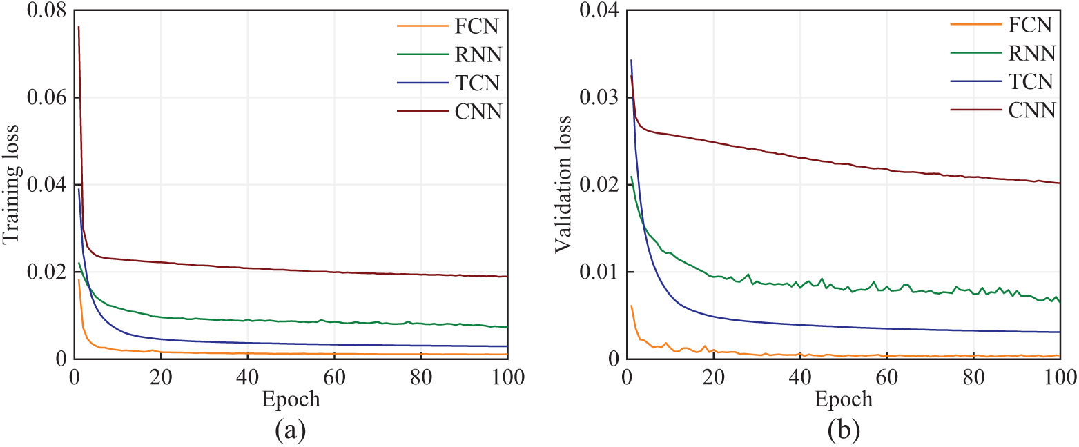
Figure 4: Loss curves: (a) training set and (b) validation set

The study compares reconstruction methods using time domain and frequency domain metrics, along with training time as a computational requirement.

The evaluation results, as depicted in Table 2 and Fig. 5, provide a detailed analysis of the performance across these metrics. Furthermore, Fig. 6 offers a visual representation of the methods’ effectiveness on randomly selected samples, demonstrating their comparative performance in both time-domain and frequency-domain. Through detailed analysis, the following conclusions can be drawn:

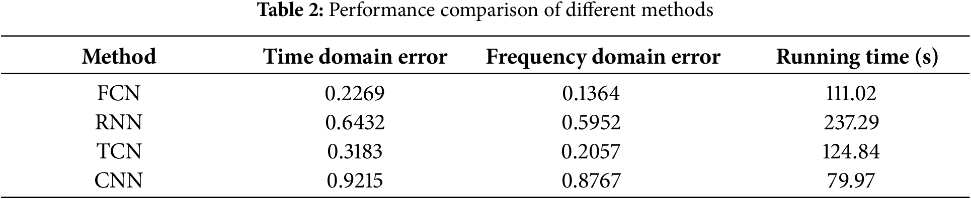
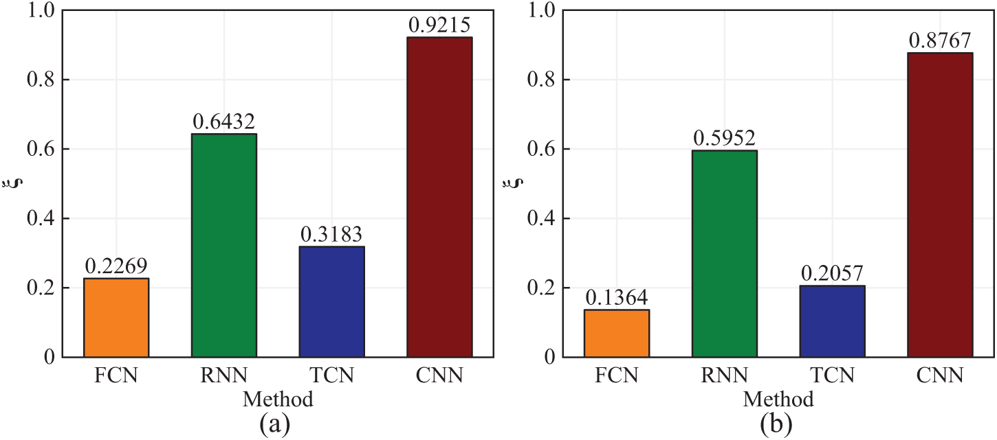
Figure 5: Comparison of response reconstruction errors across methods: (a) time domain and (b) frequency domain

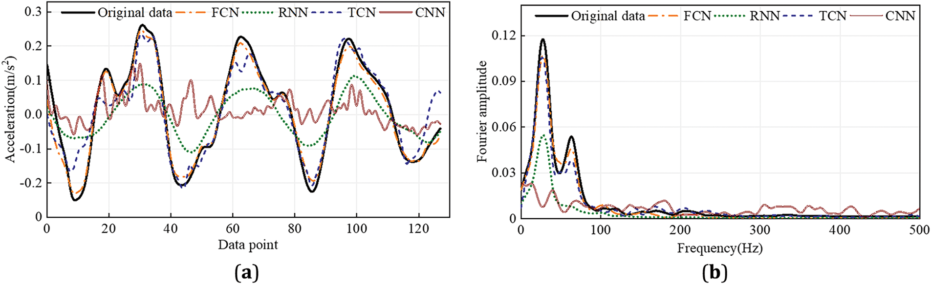
Figure 6: The reconstruction results of the samples: (a) time domain and (b) frequency domain

(1)   Compared to other networks, the proposed network has the lowest reconstruction L2 error. This is because the multi-layer structure of CNN can automatically learn features and capture multiple levels of features, whereas FCN reconstruct each high-frequency feature from abstract features, resulting in more accurate reconstructions.

(2)   As shown in Fig. 6, the acceleration response reconstructed by FCN is more consistent with the true values. The acceleration response reconstructed by TCN generally matches the overall trend of the true values but exhibits significant differences in details. The reconstruction results of RNN and CNN are less satisfactory, likely because these conventional methods cannot effectively capture high-frequency features of the data and inadequately exploit the spatiotemporal relationships in sensor data. As shown in Fig. 5, in the time domain, the proposed method’s L2 is 0.2269, which is a reduction of 64.72%, 28.71%, and 75.38% compared to the L2 values of RNN, TCN, and CNN (0.6432, 0.3183, and 0.9215, respectively). In the frequency domain, the proposed method demonstrates superior performance in signal reconstruction, as indicated by the smaller and more consistent fluctuations in the reconstructed signal. This is quantitatively supported by the L2 error value of 0.1364, which is significantly lower than those of the three other methods, with values of 0.5952, 0.2057, and 0.8767, respectively.

In summary, the FCN-based network outperforms RNN, TCN, and CNN in reconstructing bridge acceleration responses. The proposed method is not only computationally efficient but also achieves satisfactory reconstruction accuracy in both the time and frequency domains. Compared to the other three methods, the proposed method’s reconstruction results are more consistent with the original signal. As mentioned earlier, conventional methods fall short in leveraging temporal correlations in sensor data. Conversely, FCN adeptly capture both spatial and temporal correlations, enabling effective reconstruction of high-frequency acceleration response characteristics. Due to the network’s capability of extracting spatiotemporal correlations, it can reconstruct structural acceleration responses with smaller errors.

4  Practical Bridge Application

4.1 Basic Information

As shown in Fig. 7, the 1005-meter Nanji Gate Rail Transit Special Bridge in Chongqing, a double-cable semi-floating cable-stayed structure, is used to validate the proposed acceleration response reconstruction method. To ensure continuous monitoring of structural vibrations and environmental conditions, a sophisticated SHM system has been installed on the bridge. This system includes 10 uniaxial accelerometers positioned across specified span locations, which measure both vertical and transverse acceleration at a sampling rate of 50 Hz. The in-service acceleration data collected from these sensors were employed for training and testing the proposed method, enabling a comprehensive evaluation of its effectiveness.

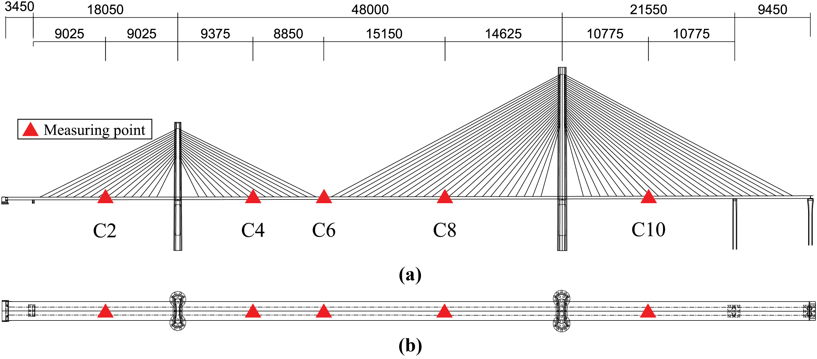
Figure 7: Schematic layout of acceleration monitoring points for the Nanji gate rail transit special bridge: (a) elevation and (b) plan view (unit: cm)

4.2 Dataset Preparation

In this study, vertical acceleration response data from five monitoring sections along the main beam, spanning from left to right, were processed for one hour. These sections were designated as channels 2, 4, 6, 8, and 10, and were used as datasets to evaluate the accuracy of the proposed method for response reconstruction. In this section, data from only two channels (i.e., C2 and C6) were used, with C6 serving as the output channel and C2 as the input channel. To prevent overfitting, the sliding window method described in Section 2.2 was employed to segment the acceleration data, with a window length and step size of 512 and 128, respectively, resulting in 1389 samples of length 512. The key parameters for this dataset are summarized in Table 3. The samples were shuffled and batched into the FCN for training and validation. In the following study, a batch size of 32 was chosen. Acceleration data with healthy channel measurements were directly input into the trained network, while the faulty channels were defined as labeled outputs.

4.3 Reconstruction Result

The model training and hyperparameter settings followed the configuration detailed in Section 3.3. Given the large sample size of the real bridge monitoring data, the learning rate and number of epochs were adjusted to 0.0005 and 200, respectively, to achieve optimal training performance.

Fig. 8 shows the loss curves during the model training process. As can be seen, the training loss and validation loss exhibit a noticeable downward trend from the beginning of the training. Due to the Adam algorithm’s ability to compute adaptive learning rates for different parameters, the loss values quickly decrease after a brief plateau period. As the training epochs accumulate, the training loss persists in declining, with the loss curve progressively stabilizing past the 150th epoch. After training is finalized, the loss for the training set is 3.34 × 10−3, and the loss for the validation set is 2.62 × 10−3. The small difference between the training error and validation error indicates that the proposed FCN can effectively reconstruct complex acceleration data from in-service bridges. Training for 200 epochs is feasible and prevents overfitting.

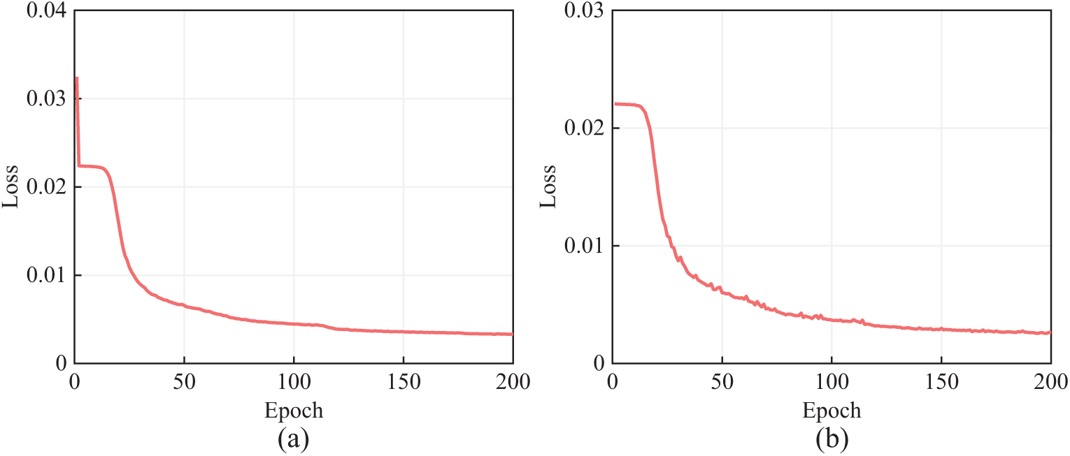
Figure 8: Training processes of FCN: (a) training; (b) validation

Fig. 9 show the comparison between the original true response and the reconstructed response of a randomly selected sample from the validation set in both the time and frequency domains. The proposed method can effectively reconstruct the acceleration response on the real bridge. In the frequency domain, the amplitude of the reconstructed signal is very close to that of the true signal. In the time domain, although some peak signals are not reconstructed with perfect consistency, the overall consistency is quite good. Overall, the signal reconstruction effect in the frequency domain is superior to that in the time domain.

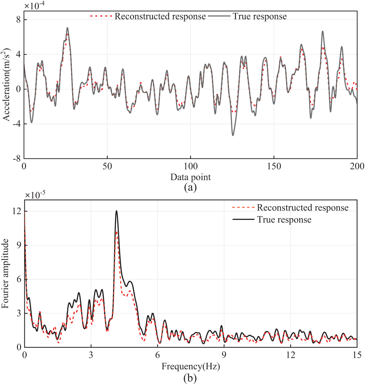
Figure 9: Response reconstruction of channel 6 based on channel 2: (a) Time domain, ξ=0.2943 and (b) Frequency domain, ξ=0.2672

5  Parametric Analysis

In this section, the performance of the proposed method under various conditions will be evaluated, such as the available response positions, the number of available channels, multi-channel response reconstruction, and sample length, in order to determine the impact of these factors on the quality of signal reconstruction.

5.1 The Effect of Input Channels Spatial Location

Following the results of using C2 as the input channel to reconstruct C6, the network was subsequently trained to reconstruct C6 using C4, C8, and C10 as input channels, respectively.

Fig. 10 illustrates the reconstructed results across various input channels. Fig. 10a displays the comparison between the reconstructed response and the original true response in the time domain at channel C6, using channels C2, C4, C8, and C10 as input channels. Fig. 10b shows the comparison between the true response and the reconstructed response in the frequency domain. Although the original data is well reconstructed using different input channels, significant differences in the reconstruction results remain evident. It is observed that when using C2 and C10 as inputs, the reconstruction error is relatively large, whereas the reconstruction error is much smaller when using channels C4 and C8 as inputs.

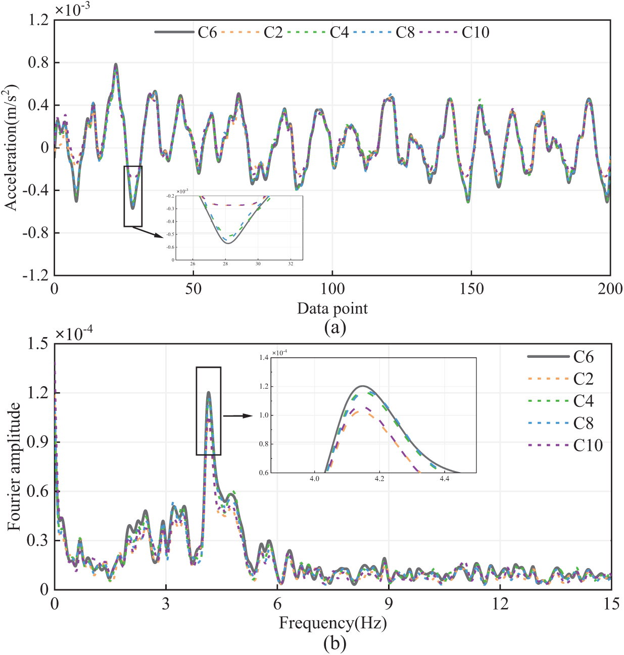
Figure 10: Response reconstruction results with different input channels: (a) Time domain and (b) Frequency domain

Fig. 11 shows the reconstruction errors in the time and frequency domains for each network on different training datasets. The reconstruction errors exhibit similar trends in both the time and frequency domains. Fig. 11 also quantitatively validates this phenomenon: when using C2 as the input, the validation set samples exhibit reconstruction errors of 0.2943 in the time domain and 0.2295 in the frequency domain, respectively. In contrast, when using C4 as the input, the validation set samples exhibit reconstruction errors of 0.2271 in the time domain and 0.1636 in the frequency domain, respectively.

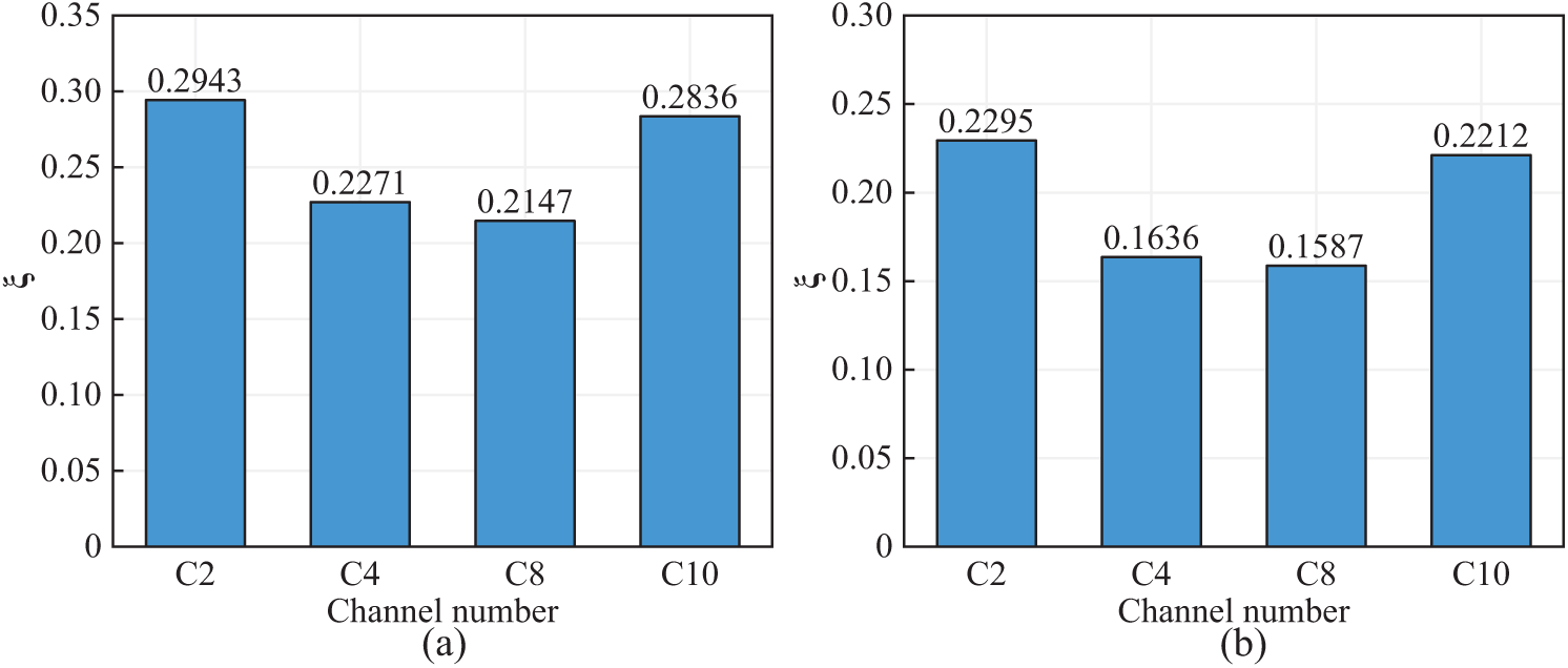
Figure 11: Reconstruction error of channel C6 using different input channels: (a) Time domain and (b) Frequency domain

To investigate the influence of input-output channel relationships on reconstruction accuracy, the study calculated the Absolute Value Correlation Coefficient (AVCC) between selected input channels (C2, C4, C8, C10) and the output channel (C6). This quantitative measure provided insight into the degree of linear association between the input and output signals. As shown in Fig. 12, scatter plots were generated to depict the connection between reconstruction errors and the corresponding AVCCs for each input channel. Analysis of these plots revealed a clear trend: as the AVCC increased, the reconstruction errors in both the time and frequency domains decreased. This finding underscores the importance of selecting input channels with higher correlation to the target output for enhancing the efficacy of the reconstruction method. The AVCC in the time domain is significantly lower than that in the frequency domain, which also confirms that the reconstruction error in the frequency domain is smaller than that in the time domain. When the input and output channels are highly correlated, the FCN more easily establishes a nonlinear mapping, leading to more satisfactory reconstruction results. Therefore, it is necessary to select input channels with high correlation to improve reconstruction accuracy.

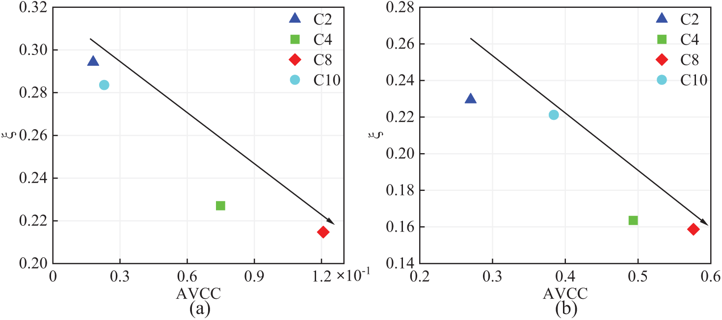
Figure 12: The connection between reconstruction errors and their respective correlation coefficients: (a) Time domain and (b) Frequency domain

5.2 The Effect of Input Channels’ NUMBER on Reconstruction Results

The effect of increasing the number of input channels on the ability to model spatio-temporal correlations between sensors is explored. Four distinct cases (S1 to S4) were examined, each incorporating a progressively larger number of input channels, ranging from 1 to 4. Table 4 outlines the specific input channels utilized in each individual case. To ensure a controlled comparison, all other network parameters were held constant across the cases, with the only variable being the network input size, which was adjusted according to the number of input channels.

Fig. 13 shows a comparison of the original and reconstructed responses in time and frequency domains. It is evident that the original signals are well reconstructed in all cases, but the reconstruction accuracy varies slightly among different cases; specifically, the more input channels, the more consistent the reconstruction results are with the original data. Fig. 14 shows that as the number of input channels increases, the reconstruction error gradually decreases. However, the improvement in reconstruction accuracy diminishes as the number of input channels grows. This implies that the FCN can form a complex nonlinear mapping with just a few input channels, allowing for accurate reconstruction of missing data.

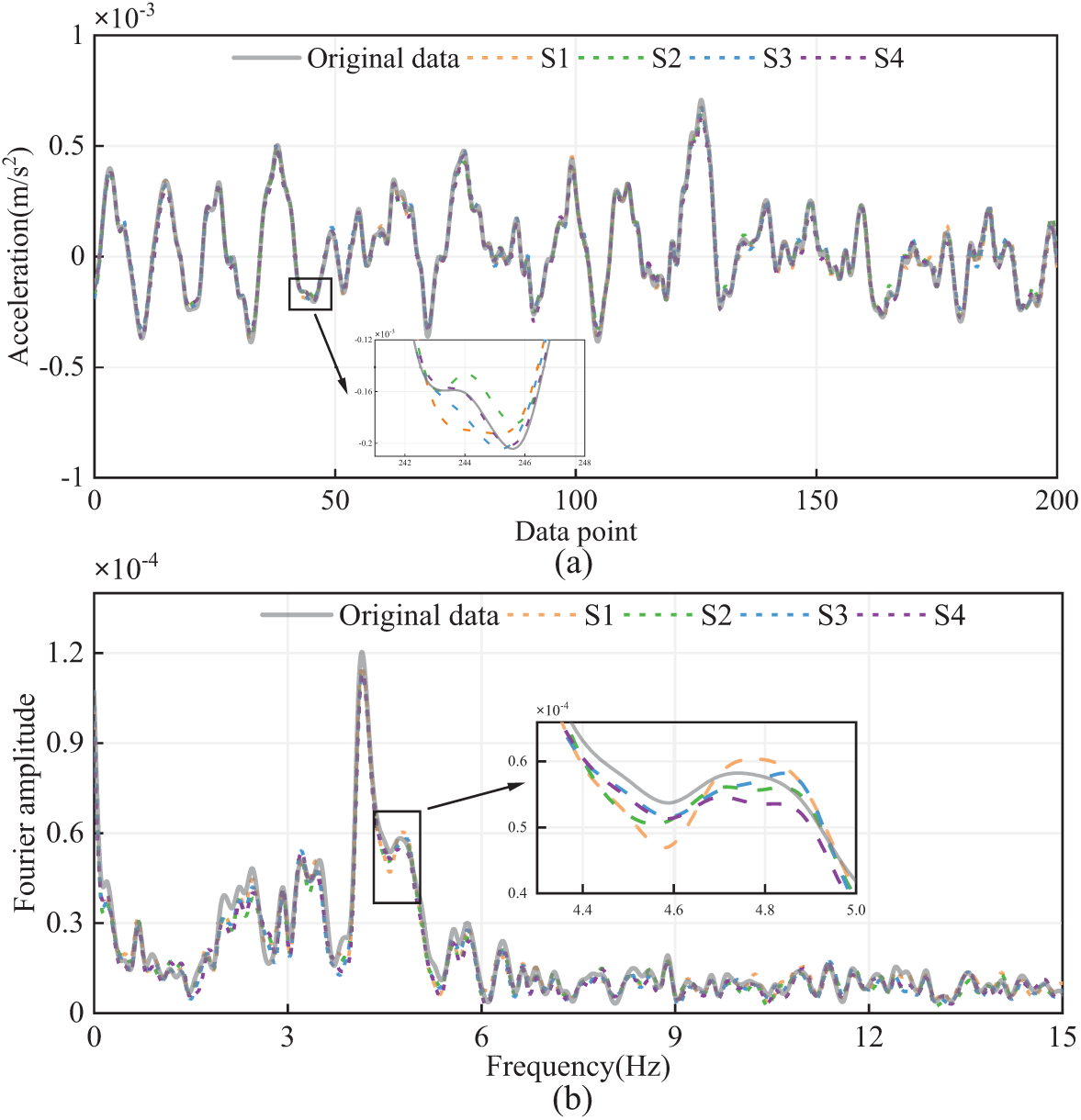
Figure 13: Different cases of multi-to-one response reconstruction: (a) Time domain and (b) Frequency domain

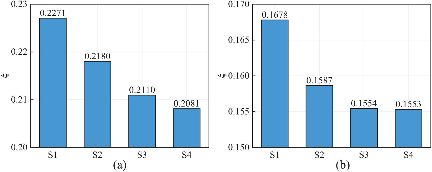
Figure 14: Error of response reconstruction in different cases: (a) Time domain and (b) Frequency domain

5.3 Multi-Channel Response Reconstruction

Multi-channel response reconstruction plays a critical role in managing simultaneous sensor failures within a SHM system. In this study, channel C6 is utilized as the input for reconstructing the responses of four output channels (i.e., C2, C4, C8, and C10). To effectively handle multi-channel data output, the number of convolution kernels in the network’s output layer is adjusted to match the number of output channels. Specifically, for this configuration, the network output is designed to accommodate four channels. All other parameter settings remain consistent with those used in prior sections.

The reconstruction results of validation samples for each output channel are shown in Fig. 15. The reconstruction results for the validation samples demonstrate a variation in accuracy across the output channels. Specifically, channels C4 and C8 exhibit higher accuracy in comparison to channels C2 and C10, where the reconstruction accuracy is relatively lower. This discrepancy in performance across different channels is further corroborated by the evaluation metrics shown in Fig. 16, which clearly highlight the differences in accuracy levels. It is evident from the figure that the time-domain error for the reconstruction results of C8 is 0.5003, the smallest error, while the time-domain error for the reconstruction results of C2 is 0.6621, the largest error. In the frequency domain, the largest reconstruction error is 0.4851 for C2, and the smallest error is 0.385 for C4. Specifically, the correlation between C4, C8, and C6 is the highest (see Fig. 12), leading to the best reconstruction accuracy. Conversely, the correlation between C2, C10 and C6 is the lowest, leading to relatively larger reconstruction errors. In general, the proposed method can reconstruct the responses of multiple target output channels using only one input channel, with larger reconstruction errors for output channels that have lower correlations with the input channel.

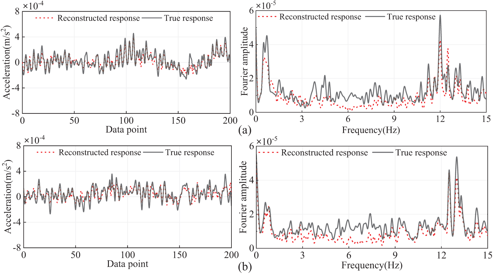
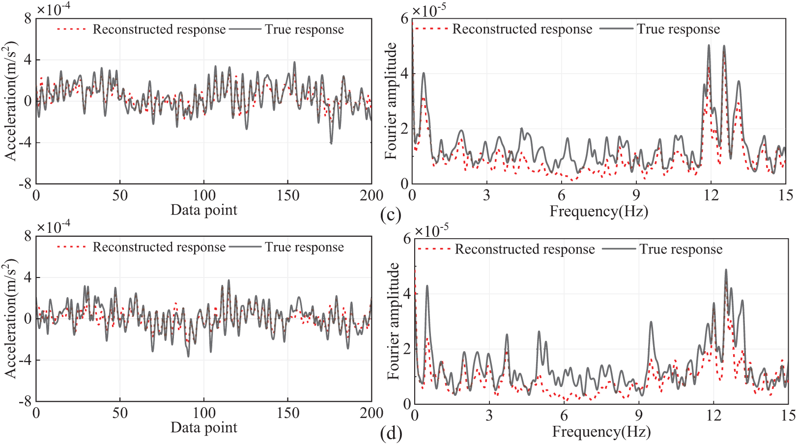
Figure 15: Comparison between true and reconstructed responses in time and frequency domains.: (a) C2; (b) C4; (c) C8; (d) C10

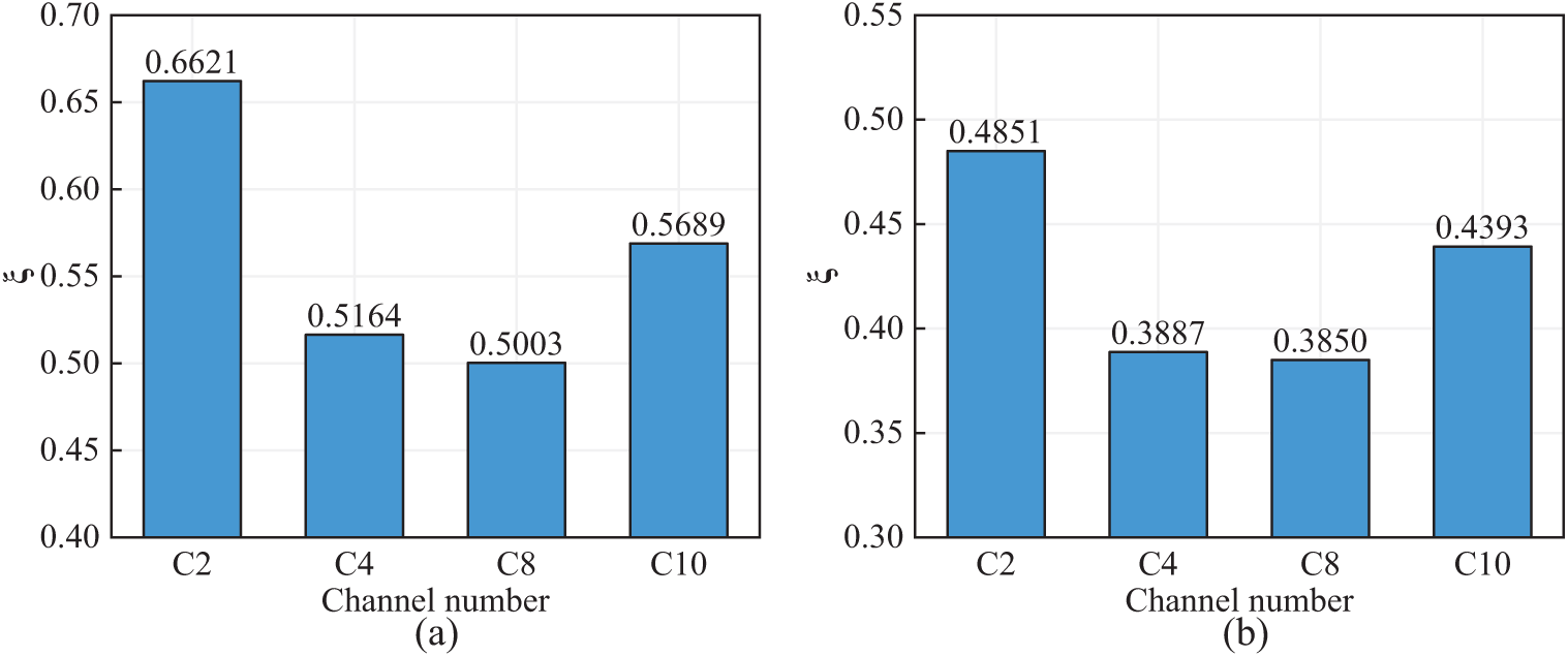
Figure 16: Error in reconstructing multi-channel responses using a single channel: (a) Time domain and (b) Frequency domain

5.4 The Influence of Sample Length on Reconstruction Results

To investigate the impact of different sample lengths on the model’s reconstruction performance, sample lengths of 64, 128, 256, and 512 were used. The acceleration data from channel C2 was used to reconstruct the data for channel C6. The results are presented in Fig. 17.

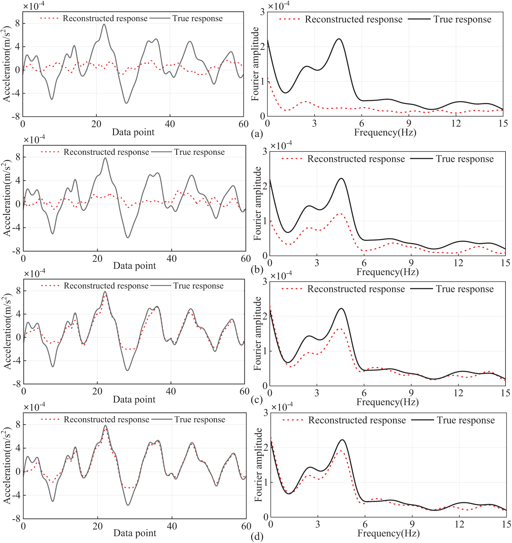
Figure 17: Reconstruction results with different sample lengths: (a) sample length 64; (b) sample length 128; (c) sample length 256; (d) sample length 512

As seen in Fig. 17 and Table 5, the reconstruction error of the model decreases with the increase in sample length. This is because when the sample length is short, the neural network model cannot learn data features effectively from the shorter data samples. In other words, there are not enough data features within each sample for the model to learn from. As the sample length increases, the training samples contain more data features, allowing the model to learn more hidden features during the training process. Consequently, this leads to improved performance in response reconstruction.

To visually present the reconstruction performance of the model across different sample lengths more intuitively, Table 5 lists the comparison of reconstruction errors.

6  Conclusion

This paper proposes an acceleration response reconstruction method for SHM based on FCN. Through the recovery of acceleration data from experimental arch ribs and the reconstruction of measured acceleration responses of long-span bridges, the following key conclusions were drawn:

(1)   The proposed FCN model effectively learns advanced features between failed and intact channels, yielding significantly lower reconstruction errors in both time and frequency domains. Compared to other models (such as CNN, RNN, and TCN), the reconstruction results of the proposed method demonstrate the highest consistency with the original signals.

(2)   Given the complex non-stationary and nonlinear characteristics of long-span bridge acceleration monitoring data, reconstruction validation using actual bridge acceleration data demonstrates that the proposed method can effectively recover missing data in practical applications. For instance, when using Channel 2 to reconstruct Channel 6 acceleration data, the L2 norm errors in the time and frequency domains are 0.2943 and 0.2672, respectively.

(3)   Benefiting from the FCN model’s strong capability to exploit spatiotemporal correlations between channels, a higher correlation between input and output channels results in a smaller reconstruction error. For instance, when reconstructing Channel 6, the L2 norm errors using Channels 2 and 8 are 0.2295 and 0.1587, respectively, with absolute correlation coefficients of 0.2699 and 0.5762 relative to Channel 6. Therefore, selecting highly correlated input channels can significantly improve recovery accuracy.

(4)   Increasing the number of input channels plays a crucial role in enhancing the modeling of spatiotemporal correlations between sensors. In cases where multiple sensors fail, multi-channel response reconstruction can still be achieved through single-channel input, with reconstruction errors related to inter-channel correlation. Choosing an appropriate sample length also aids in improving model reconstruction performance, with longer sample lengths resulting in higher reconstruction accuracy.

Although the proposed method has been validated only on the experimental arch rib and cable-stayed bridge, it is also applicable to other large-scale structures, such as buildings, tunnels, and dams. Despite its promising performance, the method has limitations, such as the need for further validation in more complex and dynamic environments, as well as across different structural types.

Acknowledgement: This work was supported by the National Natural Science Foundation of China, the Chongqing Outstanding Youth Science Foundation, the Science and Technology Project of Sichuan Provincial Transportation Department, and the Science and Technology Project of Guizhou Provincial Transportation Department.

Funding Statement: National Natural Science Foundation of China (Grant Nos. 52408314, 52278292), Chongqing Outstanding Youth Science Foundation (Grant No. CSTB2023NSCQ-JQX0029), Science and Technology Project of Sichuan Provincial Transportation Department (Grant No. 2023-ZL-03), and Science and Technology Project of Guizhou Provincial Transportation Department (Grant No. 2024-122-018).

Author Contributions: Wenda Ma: Writing—review & editing, Writing—original draft, Methodology, Validation. Qizhi Tang: Writing—review & editing, Supervision, Methodology, Formal analysis, Conceptualization, Funding acquisition. Huang Lei: Writing—review & editing, Conceptualization. Longfei Chang: Methodology, Investigation. Chen Wang: Validation, Methodology, Formal analysis, Software. All authors reviewed the results and approved the final version of the manuscript.

Availability of Data and Materials: Data will be made available on request.

Ethics Approval: Not applicable.

Conflicts of Interest: The authors declare no conflicts of interest to report regarding the present study.

References

1. Fan Y, Xin J, Yang L, Zhou J, Luo C, Zhou Y, et al. Optimization method for the length of the outsourcing concrete working plane on the main arch rib of a rigid-frame arch bridge based on the NSGA-II algorithm. Structures. 2024;59:105767. doi:10.1016/j.istruc.2023.105767. [Google Scholar] [CrossRef]

2. Zhou Y, Cai W, Chi M, Liang S, Xu W. An improved vehicle dynamic load identification method with optimal sensor placement strategy based on augmented Kalman filter. Mech Syst Signal Process. 2025;225(12):112234. doi:10.1016/j.ymssp.2024.112234. [Google Scholar] [CrossRef]

3. Nicoletti V, Quarchioni S, Amico L, Gara F. Assessment of different optimal sensor placement methods for dynamic monitoring of civil structures and infrastructures. Struct Infrastruct Eng. 2024;2768(1):1–16. doi:10.1080/15732479.2024.2383299. [Google Scholar] [CrossRef]

4. Yang J, Huang L, Tong K, Tang Q, Li H, Cai H, et al. A review on damage monitoring and identification methods for arch bridges. Buildings. 2023;13(8):1975. doi:10.3390/buildings13081975. [Google Scholar] [CrossRef]

5. Zhang XH, Wu ZB. Dual-type structural response reconstruction based on moving-window Kalman filter with unknown measurement noise. J Aerosp Eng. 2019;32(4):4019029. doi:10.1061/(asce)as.1943-5525.0001016. [Google Scholar] [CrossRef]

6. Xu YL, Zhang XH, Zhu S, Zhan S. Multi-type sensor placement and response reconstruction for structural health monitoring of long-span suspension bridges. Sci Bull. 2016;61(4):313–29. doi:10.1007/s11434-016-1000-7. [Google Scholar] [CrossRef]

7. Zhang XH, Zhu Z, Yuan GK, Zhu S. Adaptive mode selection integrating Kalman filter for dynamic response reconstruction. J Sound Vib. 2021;515(1):116497. doi:10.1016/j.jsv.2021.116497. [Google Scholar] [CrossRef]

8. Zhu Z, Lu J, Zhu S. Multi-rate Kalman filtering for structural dynamic response reconstruction by fusing multi-type sensor data with different sampling frequencies. Eng Struct. 2023;293(1):116573. doi:10.1016/j.engstruct.2023.116573. [Google Scholar] [CrossRef]

9. Fan G, He Z, Li J. Structural dynamic response reconstruction using self-attention enhanced generative adversarial networks. Eng Struct. 2023;276:115334. doi:10.1016/j.engstruct.2022.115334. [Google Scholar] [CrossRef]

10. Wan HP, Ni YQ. Bayesian multi-task learning methodology for reconstruction of structural health monitoring data. Struct Health Monit. 2019;18(4):1282–309. doi:10.1177/1475921718794953. [Google Scholar] [CrossRef]

11. Bao Y, Shi Z, Wang X, Li H. Compressive sensing of wireless sensors based on group sparse optimization for structural health monitoring. Struct Health Monit. 2018;17(4):823–36. doi:10.1177/1475921717721457. [Google Scholar] [CrossRef]

12. Bao Y, Tang Z, Li H. Compressive-sensing data reconstruction for structural health monitoring: a machine-learning approach. Struct Health Monit. 2020;19(1):293–304. doi:10.1177/1475921719844039. [Google Scholar] [CrossRef]

13. Wan HP, Dong GS, Luo Y, Ni YQ. An improved complex multi-task Bayesian compressive sensing approach for compression and reconstruction of SHM data. Mech Syst Signal Process. 2022;167(4):108531. doi:10.1016/j.ymssp.2021.108531. [Google Scholar] [CrossRef]

14. Cha YJ, Ali R, Lewis J, BüyükÖztürk O. Deep learning-based structural health monitoring. Autom Constr. 2024;161(3):105328. doi:10.1016/j.autcon.2024.105328. [Google Scholar] [CrossRef]

15. Abdeljaber O, Avci O, Kiranyaz S, Gabbouj M, Inman DJ. Real-time vibration-based structural damage detection using one-dimensional convolutional neural networks. J Sound Vib. 2017;388:154–70. doi:10.1016/j.jsv.2016.10.043. [Google Scholar] [CrossRef]

16. Xin J, Zhou J, Zhou F, Yang SX, Zhou Y. Bearing capacity model of corroded RC eccentric compression columns based on Hermite interpolation and Fourier fitting. Appl Sci. 2019;9(1):24. doi:10.3390/app9010024. [Google Scholar] [CrossRef]

17. Lin YZ, Nie ZH, Ma HW. Structural damage detection with automatic feature-extraction through deep learning. Comput Aided Civil Eng. 2017;32(12):1025–46. doi:10.1111/mice.12313. [Google Scholar] [CrossRef]

18. Wang Z, Cha YJ. Unsupervised deep learning approach using a deep auto-encoder with a one-class support vector machine to detect damage. Struct Health Monit. 2021;20(1):406–25. doi:10.1177/1475921720934051. [Google Scholar] [CrossRef]

19. Fan G, Li J, Hao H. Dynamic response reconstruction for structural health monitoring using densely connected convolutional networks. Struct Health Monit. 2021;20(4):1373–91. doi:10.1177/1475921720916881. [Google Scholar] [CrossRef]

20. Fan G, Li J, Hao H, Xin Y. Data driven structural dynamic response reconstruction using segment based generative adversarial networks. Eng Struct. 2021;234:111970. doi:10.1016/j.engstruct.2021.111970. [Google Scholar] [CrossRef]

21. Jeong S, Ferguson M, Hou R, Lynch JP, Sohn H, Law KH. Sensor data reconstruction using bidirectional recurrent neural network with application to bridge monitoring. Adv Eng Inform. 2019;42(3):100991. doi:10.1016/j.aei.2019.100991. [Google Scholar] [CrossRef]

22. Wang ZW, Lu XF, Zhang WM, Fragkoulis VC, Beer M, Zhang YF. Deep learning-based reconstruction of missing long-term girder-end displacement data for suspension bridge health monitoring. Comput Struct. 2023;284:107070. doi:10.1016/j.compstruc.2023.107070. [Google Scholar] [CrossRef]

23. Oh BK, Glisic B, Kim Y, Park HS. Convolutional neural network-based data recovery method for structural health monitoring. Struct Health Monit. 2020;19(6):1821–38. doi:10.1177/1475921719897571. [Google Scholar] [CrossRef]

24. Ijjeh AA, Ullah S, Kudela P. Full wavefield processing by using FCN for delamination detection. Mech Syst Signal Process. 2021;153:107537. doi:10.1016/j.ymssp.2020.107537. [Google Scholar] [CrossRef]

25. Chaiyasarn K, Buatik A, Mohamad H, Zhou M, Kongsilp S, Poovarodom N. Integrated pixel-level CNN-FCN crack detection via photogrammetric 3D texture mapping of concrete structures. Autom Constr. 2022;140(4):104388. doi:10.1016/j.autcon.2022.104388. [Google Scholar] [CrossRef]

26. Wang Z, Gao X, Wu R, Kang J, Zhang Y. Fully automatic image segmentation based on FCN and graph cuts. Multimed Syst. 2022;28(5):1753–65. doi:10.1007/s00530-022-00945-3. [Google Scholar] [CrossRef]

27. Shelhamer E, Long J, Darrell T. Fully convolutional networks for semantic segmentation. IEEE Trans Pattern Anal Mach Intell. 2017;39(4):640–51. doi:10.1109/TPAMI.2016.2572683. [Google Scholar] [PubMed] [CrossRef]

28. Lei X, Sun L, Xia Y. Lost data reconstruction for structural health monitoring using deep convolutional generative adversarial networks. Struct Health Monit. 2021;20(4):2069–87. doi:10.1177/1475921720959226. [Google Scholar] [CrossRef]

29. Srivastava N, Hinton G, Krizhevsky A, Sutskever I, salakhutdinov R. Dropout: a simple way to prevent neural networks from overfitting. J Mach Learn Res. 2014;15(56):1929–58. [Google Scholar]

30. He K, Zhang X, Ren S, Sun J. Delving deep into rectifiers: surpassing human-level performance on ImageNet classification. In: 2015 IEEE International Conference on Computer Vision (ICCV); 2015 Dec 7–13; Santiago, Chile. p. 1026–34. doi:10.1109/ICCV.2015.123. [Google Scholar] [CrossRef]