Diff-Fastener: A Few-Shot Rail Fastener Anomaly Detection Framework Based on Diffusion Model

1  Introduction

Railroad fasteners are key components of the railroad system and play a critical role in maintaining the stability of rail connections and ensuring safety during operation. However, due to long-term use and the influence of external environmental factors, railroad fasteners may experience abnormalities such as missing and damaged parts, which may lead to railroad accidents and operational failures [1]. Therefore, timely and accurate inspection of railroad fasteners is crucial.

However, anomaly detection methods based on supervised learning are limited by the number of samples and perform poorly with unbalanced data. Therefore, unsupervised anomaly detection methods based on unsupervised learning have wider applicability.

Unsupervised anomaly detection models are mainly divided into two types: feature embedding-based models and generative model-based models. PatchCore [2] is an advanced method for anomaly detection that utilizes feature embedding. This model extracts local features from images and uses a memory bank to store the features of normal samples, allowing it to compare the differences between abnormal regions and normal features during the detection process. RD++ (Reversed Distillation++) [3] introduces more complex feature fusion strategies and optimization algorithms, enabling it to capture subtle anomalous information better, making it suitable for high-dimensional and complex anomaly detection tasks. SimpleNet [4] is a simplified feature embedding model designed to enhance computational efficiency by reducing model complexity. FastFlow [5] utilizes flow-based generative models for anomaly detection. DRAEM (Discriminatively trained Reconstruction Anomaly Embedding Model) [6] combines denoising autoencoders with reconstruction methods to detect anomalies by denoising and reconstructing input data. Its innovation lies in its dual reconstruction mechanism, which allows for more accurate identification of anomalous regions while maintaining high-fidelity reconstruction of normal data.

Recently, diffusion modeling has been explored in the field of anomaly detection [7–10]. DDPM (Denoising Diffusion Probabilistic Model) [11] demonstrates competitive effectiveness relative to preceding unsupervised and semi-supervised anomaly detection methodologies. It does not require labelled anomalous samples for training, while also exhibiting strong robustness, allowing it to be flexibly applied to different types of data, including images, time series, texts, etc. DDAD (Denoising Diffusion Anomaly Detection) [12] provides a conditional denoising process to generate anomaly-free images that are similar to the target image, improving inference speed while maintaining equivalent anomaly detection performance. Within the realm of healthcare, denoising diffusion models have been employed in the identification of brain tumors [13,14]. AnoDDPM [15] developed a multi-scale simplex noise diffusion process capable of controlling the target anomaly size. DiAD [16] is a diffusion-based framework containing a semantic bootstrap module and a spatial-aware feature fusion module, which solves the problem of category and semantic loss in Stable Diffusion multi-class anomaly detection. DefectFill [17] fine-tunes the repair diffusion model to produce realistic and high-fidelity defect images with limited reference samples. DiffusionAD [18] consists of a reconstruction sub-network, which uses Residual U-Net to reformulate the reconstruction process as a noise-to-normal paradigm, and a segmentation sub-network, which utilizes the input graphs and their anomaly-free recovery results to predict the pixel-level anomaly scores, and is experimentally shown to outperform the current state-of-the-art (SOTA) methods.

Nevertheless, the enhanced expressiveness and interpretability of the DDPM incur significant computational expenses. Such computational intricacy poses obstacles for anomaly detection endeavors encompassing extensive datasets or continuous data streams. Additionally, one of the key components in diffusion models is the U-Net used for noise prediction, continuous downsampling results in reduced resolution and thus, degradation of fine details. The contributions of this paper can be summarized as follows:

(1)   To the best of our knowledge, this work introduces a diffusion model to the rail fastener anomaly detection task for the first time, named Diff-Fastener. It requires only a small number of normal samples in the training phase, and uses an anomaly synthesis strategy to convert half of the normal samples into anomalous samples online. This feature not only reduces the dependence on the amount of anomaly data but also significantly enhances the model’s ability to detect unknown anomalies.

(2)   This work employs one-step denoising to improve the efficiency of image reconstruction, while using a Norm-Guided strategy to alleviate the excessive smoothing problem it brings. The reconstruction results of anomalous regions obtained at relatively large noise scales are utilized to guide the reconstruction at smaller noise scales to improve the accuracy of the reconstruction.

(3)   We propose a module, DACM, used in the middle layer of the reconstructed network to filter and weight the features and increase the receptive field. Sparse-Skip connections are used instead of the original dense skip connections to reduce the computational load of the model and improve scalability, and all activation functions are replaced with GELU (Gaussian Error Linear Unit). Finally, we perform exhaustive experiments on the MVTec, VisA, and railroad fastener datasets.

2  Preliminaries

2.1 Diffusion Models

Diffusion models [11,19,20] represent a category of generative models that draw inspiration from the principles of nonequilibrium thermodynamics. They establish a framework wherein the forward process incrementally introduces random noise into the data, whereas the reverse process systematically generates the targeted data samples from noise.

2.1.1 Diffusion Process

The diffusion process entails the incremental alteration of the original image x0 into xT by incrementally adding Gaussian noise, thereby achieving the goal of corrupting the image. This process is also known as the forward (positive) noise addition process, which the formula can represent:

xt=xt−1αt+ϵt−11−αt,ϵt−1∼N(0,1)(1)

This process transforms the data sample x0 into a noise sample xt, where t is randomly drawn from {0,1,…,T}, ϵt−1∼N(0,1) represents Gaussian noise, and {αt}t=1T are predefined hyperparameters, known as the noise schedule. These αt values are crucial as they control the variance of the noise added at each step. A higher αt implies less noise addition, preserving more of the original image’s characteristics at step t, while a lower αt means more noise is introduced, rapidly transforming the image towards a pure noise state. Typically, αt is set in a decreasing sequence, often following a linear or cosine-based schedule, to ensure a smooth transition from the original image to noise. The choice of the αt schedule significantly impacts the model’s ability to learn the underlying data distribution; a well-designed schedule can facilitate better convergence during training and improve the quality of generated samples.

By iteratively deriving from the above formula, we can obtain the direct transformation formula from x0 to xt as follows:

xt=x0α¯t+ϵt1−α¯t,ϵt∼N(0,1)(2)

given that α¯t=∏i=0tαi, which is a hyperparameter set according to the noise schedule, and ϵt∼N(0,1) is also Gaussian noise. Both Eqs. (1) and (2) can describe the forward noise addition process, with the former used for gradually corrupting an image and the latter for corrupting an image in one step.

2.1.2 Reverse Process

The diffusion process encompasses the addition of noise to the image, whereas the reverse process engages in denoising. Knowing the true distribution of each step in the reverse process, denoted as q(xt−1|xt), and beginning with random noise xt∼N(0,1), a gradual denoising procedure can yield an authentic sample. The parameter βt, related to αt through βt=1−αt, plays a significant role in the reverse process. A larger βt implies a more aggressive denoising step, which might introduce more variance in the generated samples but could also lead to faster convergence towards the original data distribution. In the reverse process equation:

xt−1=1αt(xt−1−αt1−α¯tϵθ(xt,t))+β~tz,z∼N(0,1)(3)

given β~t=1−α¯t−11−α¯tβt. Since the real noise ϵt in the forward process equations is not allowed to be used during the restoration process, the key is to obtain a model ϵθ(xt,t) that predicts the noise from xt and t, where θ represents the training parameters of the model, and z∼N(0,1) is another Gaussian noise used to represent the difference between the prediction and the actual noise. The balance between αt and βt in the reverse process determines the stability and quality of the generated output, with improper choices potentially leading to blurry or inconsistent results.

2.2 How to Train

To estimate the distribution q(xt−1|xt), the entire training sample is required. We can estimate these distributions using neural networks. Although the derivation behind diffusion models is complex, the optimization goal we ultimately obtain is very straightforward: to make the noise predicted by the network consistent with the actual noise. During the training process, the following loss function is minimized by fitting through a Residual U-Net structure to predict ϵ:

ℒ=Et∼[1−T],x0∼q(x0),ϵ∼N(0,I)[‖ϵ−ϵθ(xt,t)‖2].(4)

3  Preliminaries

3.1 Network Structure

The core components of Diff-Fastener are the reconstruction network and the segmentation network. Both the reconstruction network and the segmentation network have U-Net as their core. A workflow of Diff-Fastener is presented in Fig. 1.

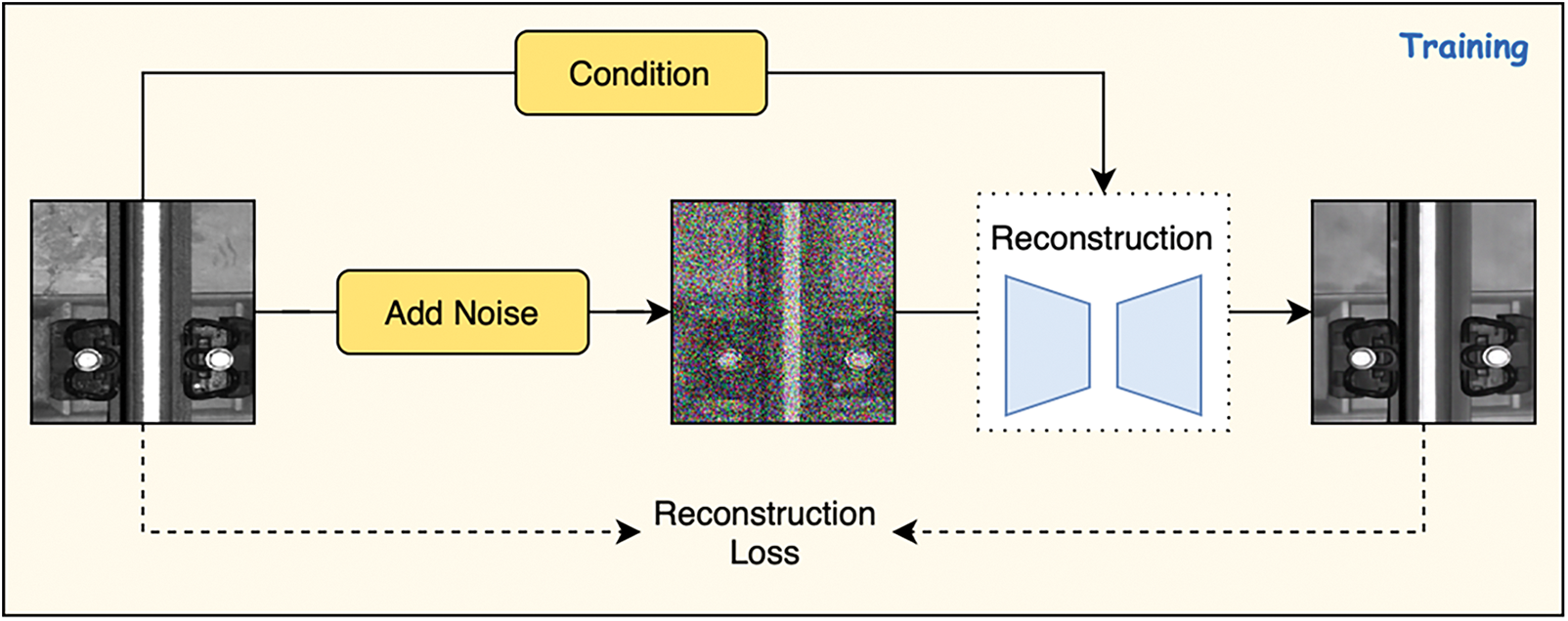
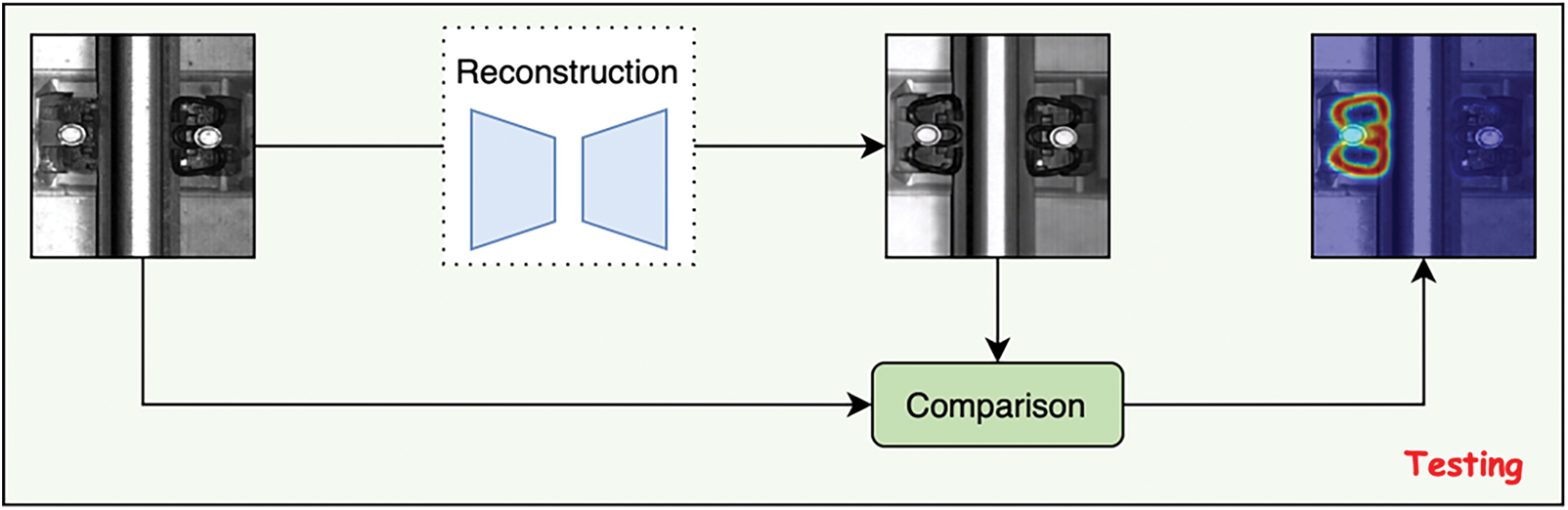
Figure 1: Workflow diagram of Diff-Fastener. After the original images are input into the model, they are disturbed by Gaussian noise. Through training, the model predicts the noise, and testing is used to learn how to reconstruct the original images. During the inference stage, the diffusion model reconstructs images of abnormal components, and by pixel matching, compares the reconstructed images with the original images to generate accurate anomaly heatmaps

3.1.1 Reconstruction Model

The reconstruction network is designed to predict the noise ε related to xt and t, based on a U-Net-like architecture integrating ResNet [21], PixelCNN++ [22], and Transformer [23]. In the noise prediction module, the encoder uses ResNet blocks with skip connections for hierarchical feature extraction, the middle layers adopt PixelCNN++ to model pixel-level spatial dependencies, and the decoder incorporates Transformer layers to capture long-range dependencies. For the module-to-module collaboration, U-Net’s skip connections transfer low-level details from the encoder to the decoder, enabling the decoder to combine high-level semantics with fine-grained information. ResNet, PixelCNN++, and Transformer components work together to enhance feature representation, refinement and synthesis. The choice of this combination is theoretically justified as U-Net suits detail recovery, ResNet boosts representational power, PixelCNN++ captures local structure, and Transformer overcomes the limitation of convolutional layers in long-range dependency modeling, achieving a balance between local and global understanding for better noise prediction.

In addition to using a U-Net-like structure as the backbone, each block in the decoder is connected to its corresponding encoder block through skip connections. Early diffusion works [24,25] have demonstrated the importance of skip connections in this architecture. On the one hand, in the encoder-decoder structure, they reduce the information loss during the downsampling process by directly passing the feature maps to the decoder, thus enriching its representation. On the other hand, skip connections accelerate the training process and improve the generation quality by providing additional gradient paths and preserving important features, enabling more efficient and effective diffusion modelling. However, the dense block-wise skip connections have become a bottleneck. A large number of block-wise skip features have to be concatenated to the features and merged along the channel dimension within the corresponding decoder blocks, which consumes excessive computational costs. Such inefficiency hinders the scalability of the model. To address this issue, we propose Sparse-Skip connections, in which the skip connections are applied only every few blocks instead of after each block. This approach improves the performance, and our experiments show that, compared with the densely connected skip design, it indeed yields better results. Fig. 2 illustrates the differences between the two U-Net structures.

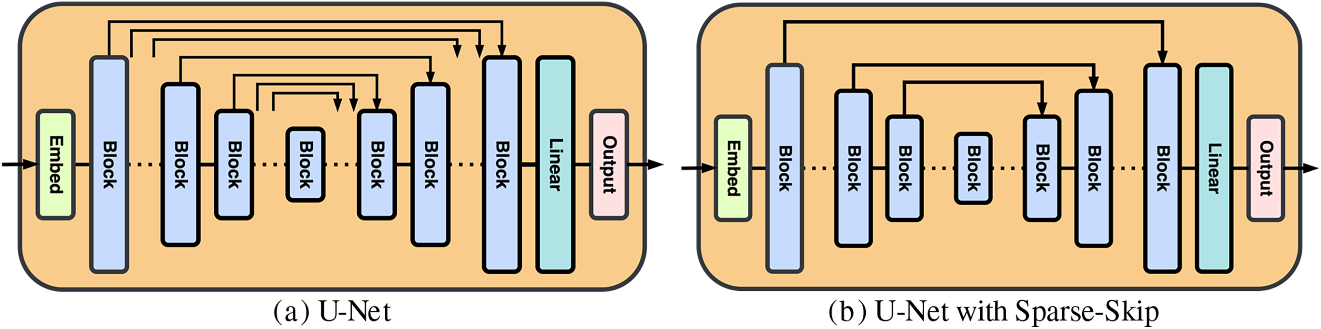
Figure 2: U-Net with different numbers of skip connections

Initially, the input image x0 is corrupted at a random time step t during the diffusion process, resulting in xt as per Eq. (2). As the time step increases, the input image x0 gradually loses its distinctive features—the anomalous pixels lose their sharp characteristics and approach an isotropic Gaussian distribution, where x0 represents a normal image or a composite abnormal image. Based on this, the reconstruction network can iteratively obtain the reconstructed anomaly-free x^0 through Eq. (3).

3.1.2 Segmentation Model

The segmentation model, based on U-Net, identifies and classifies each pixel in the image as normal or abnormal, thus achieving precise segmentation of the anomalous areas. It compares the reconstructed image x^0 with the original image x0 and learns to detect anomalies by learning the commonalities and differences between them.

3.2 One-Step Denoising

Although diffusion models possess excellent density estimation capabilities and high sampling quality, classical diffusion models generally require 50–1000 iterations, and each iteration corresponds to a round of network inference. Although this multi-step iterative method can gradually refine the reconstruction and ensure high-quality output, the calculation cost is extremely high, resulting in a very slow reasoning speed, which makes it difficult to meet the requirements of real-time application of fastener detection. To address this issue, based on the direct reconstruction using the DDPM [11] theory, we adopt one-step denoising as an alternative to iterative denoising:

x^0=1α¯t(xt−1−α¯tϵθ(xt,t))(5)

x^0 is the anomaly-free reconstruction achieved through one-step denoising. Simply put, at any time step t, once the diffusion model predicts the noise ϵθ(xt,t) for xt through a single-step inference, direct recovery is always effective. By gradually adding noise and employing one-step denoising, it effectively simulates the distribution of normal data while significantly improving inference speed. Compared to Eq. (3), this direct prediction method is t times faster than iterative prediction.

3.3 Norm-Guided Paradigm

In one-step denoising, the noise prediction of the model is completed at one time and cannot be corrected many times, which may lead to insufficient reconstruction of the details of the model, especially in the case of large noise scales. If the model’s prediction of noise is wrong, this error will directly affect the result of reconstruction and may lead to fastener image distortion, which is more obvious in images containing complex abnormal features, resulting in residual abnormal features.

Experiments have proven that different scales of noise injection are required to repair anomalies of different sizes. Larger abnormal areas require larger-scale noise to disturb, and smaller or non-existent abnormal areas require smaller-scale noise. But large-scale noise may introduce distortion, and some anomalous regions will be left when the diffusion model is used for prediction. Although small-scale noise is difficult to disturb large-area anomalies, it exhibits higher pixel quality and preserves more image details.

To take full advantage of these two noise scales, we use the Norm-Guided paradigm [18] to guide the denoising process of the diffusion model. Specifically, large-scale noise is injected into the original image and denoised to obtain the reconstructed image xb. Then, small-scale noise is injected into the original image and denoised under the guidance of xb to obtain the final reconstructed image xs. In this way, xs not only carries out a good reconstruction of anomalies in large areas, but also fully retains the details of the original image. See Fig. 3 for detailed steps.

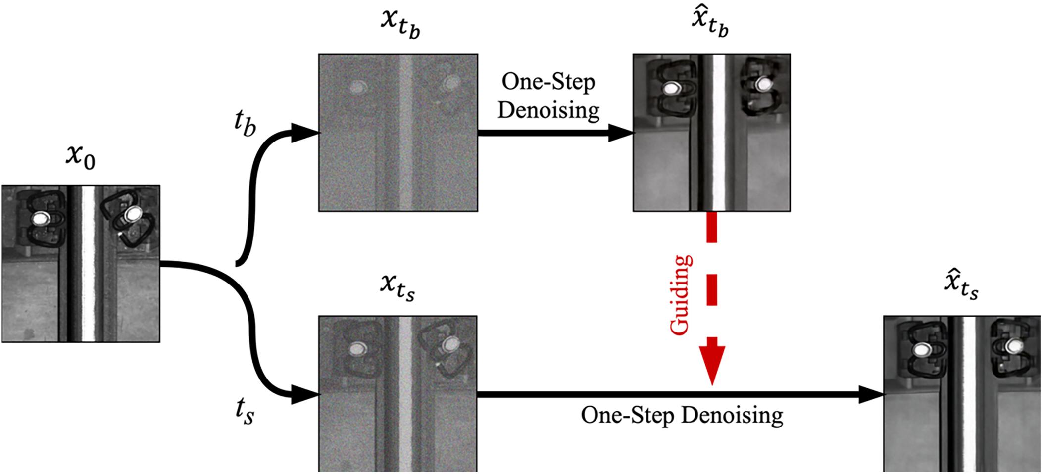
Figure 3: Norm-guided paradigm

We divide the random range of t∈{0,1,…,T} into two parts using τ, where S={0,1,…,τ} and B={τ+1,τ+2,…,T}. For an input image x0, we first perturb it using two randomly sampled time steps ts∈S and tb∈B to obtain xts and xtb through Eq. (1). Then, we use the diffusion model to predict the noise of xtb through Eq. (5), and generate a reconstructed image x^0b, denoted by n. Then, under the guidance of x^0b, we use the diffusion model to predict the noise of xts and denoise xts, bringing xts and ϵθ(xts,nts) into Eq. (5), which yields Eq. (6):

x^0s=1α¯ts(xts−1−α¯tsϵθ(xts,nts))(6)

finally generate the reconstructed image x^0s. x^0s performs well in the reconstruction of large abnormal areas and retains the rich details of the original image.

We can see from Fig. 4 that before using the norm-guided paradigm, the One-Step denoising model lacked a grasp of detailed information, and the reconstructed abnormal fastener with a distorted shape occurred after the displacement was reconstructed. After using the norm-guided paradigm, the reconstructed image showed obvious improvement in detailed information, with a more natural coupling shape and a texture on the rail that was closer to the real state.

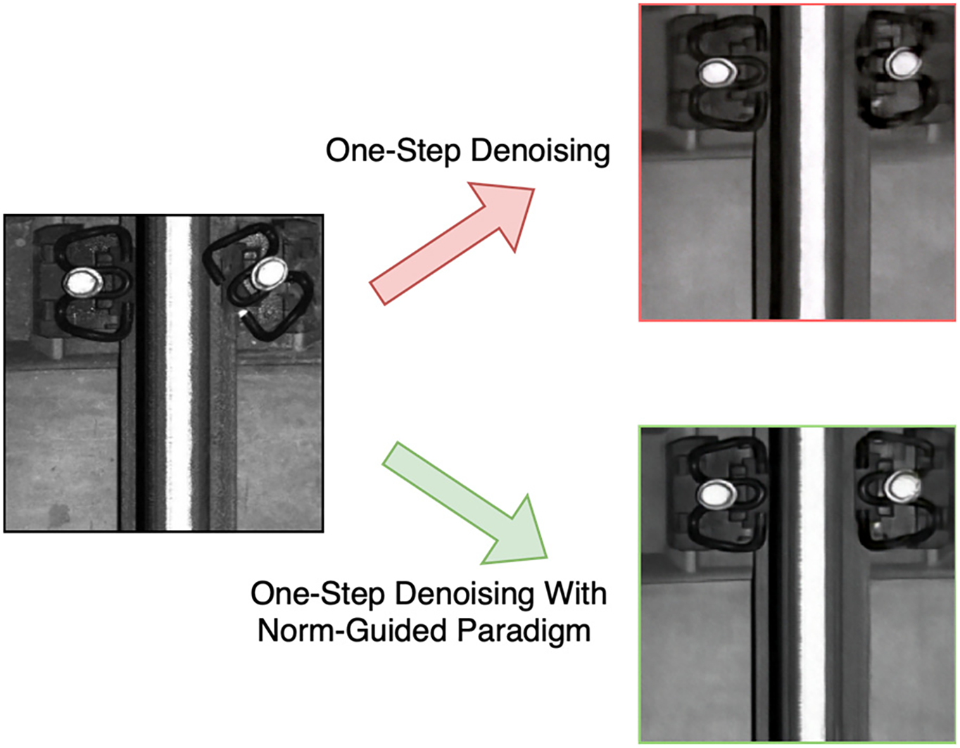
Figure 4: A comparison of the results before and after using the norm-guided paradigm

3.4 DACM

In the face of various situations such as fastener damages of different degrees, complex backgrounds, and harsh acquisition environments, even a powerful network like the residual U-Net network is prone to problems such as unstable performance and reduced generalization ability when dealing with complex and diverse datasets. Therefore, we propose a module named DACM. Experiments have proven that the introduction of DACM can effectively alleviate such problems, especially with remarkable effects in improving accuracy and restoring details.

The DACM module integrates the attention module and dilated convolutions. The former deals with the channel distribution of the feature map and helps the neural network to focus on key pixel regions while ignoring irrelevant parts. The dilated convolution with a kernel size of 3, a dilation rate of 2, and a padding of 2 in the middle layer expands the receptive field without losing spatial resolution to retain more details [26]. It solves the problem of the loss of fastener detail features caused by multiple downsamplings without increasing the number of parameters, provides richer contextual information, and enhances the model’s understanding of complex relationships. In addition, the DACM allows for the adjustment of the dilation rate to enable the model to flexibly adapt to feature detection at different granularities, significantly improving performance in complex scenarios. Fig. 5 shows our DACM.

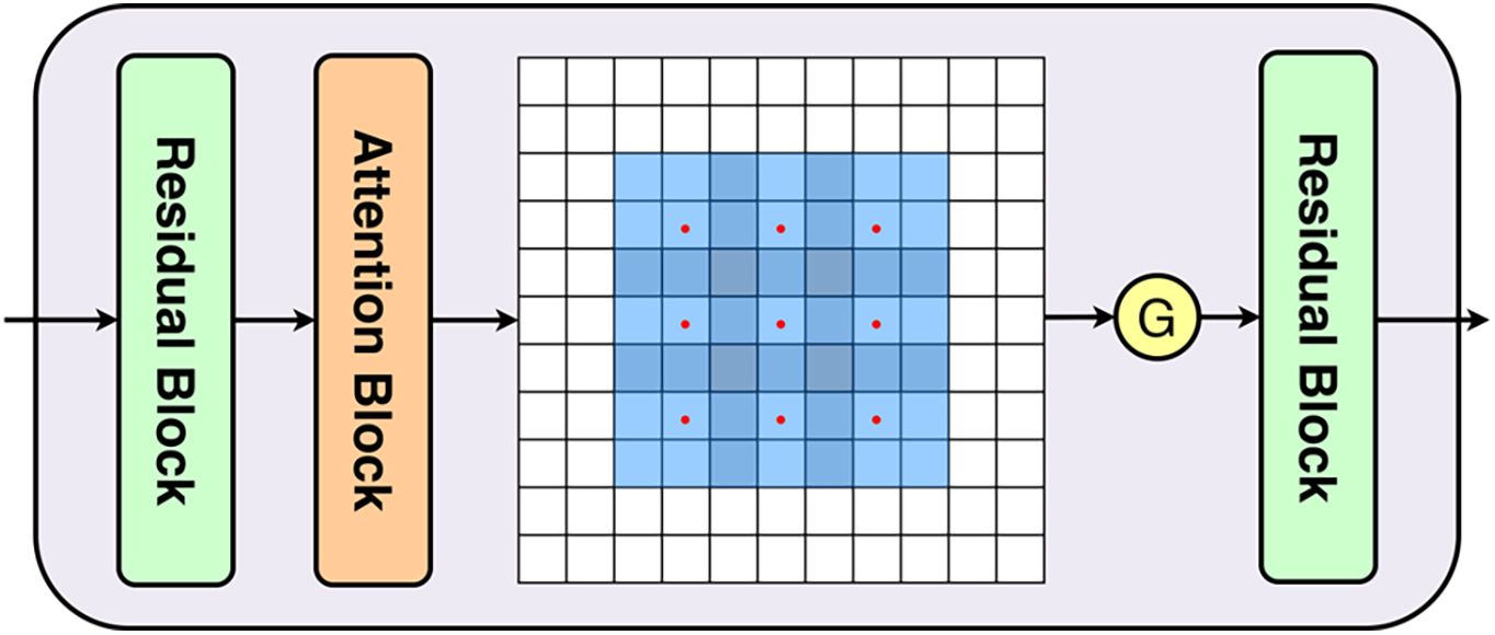
Figure 5: Structure of DACM. Wherein, “G” refers to the GELU activation function

3.5 Abnormal Fastener Synthesis Strategy

To train the model for detecting abnormal fasteners, in practical applications, we usually lack sufficient labeled samples of abnormal fasteners. Inspired by [27,28], we adopt an anomaly synthesis strategy to synthesize forged anomaly railway fastener images online, enabling the model to be trained without real anomaly samples. Specifically, our synthesis strategy is to generate areas that resemble actual anomalies by adding inconsistent visual perturbations to the normal fastener images. These forged abnormal areas are defined as “out-of-distribution” areas that simulate the different types of defects that fasteners can have in the real world.

In addition to the above-mentioned methods, we have replaced all the activation functions with GELU. The overall structure of Diff-Fastener is shown in Fig. 6, which primarily divides the anomaly detection of rail fasteners into three steps. The first step is data collection and preprocessing, where images of fasteners are collected on a railway image acquisition device and labelled with ground truth on a computer. The second step involves using Diff-Fastener for anomaly detection; the model only requires normal fastener images as input. Initially, the model will transform half of the normal images into anomalous images using an abnormal fastener synthesis strategy, and then, in combination with One-Step denoising and Norm-Guided paradigm, it will detect the fasteners. The final step is data visualization, where the model displays the detection results using heatmaps, making it easier for people to observe the results.

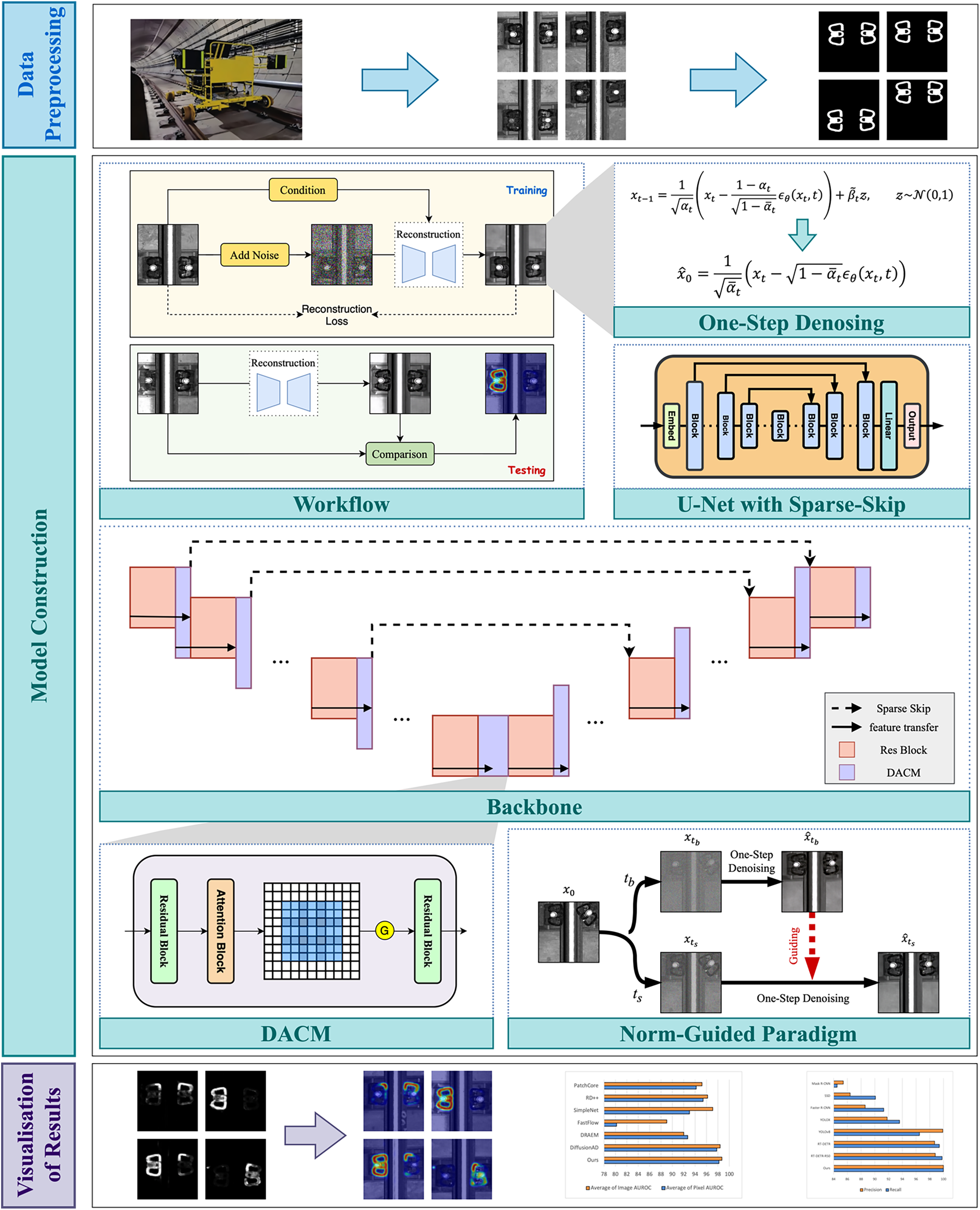
Figure 6: The overall framework of Diff-Fastener

4  Experiments

4.1 Datasets

The railway image acquisition device used in this study is shown in Fig. 7. The device can adapt to the data collection of tracks with normal gauge, and the collected image field of view includes the rails on both sides and the fasteners. The test route was a certain section of the high-speed ballastless track between Beijing and Shanghai. The basic states of the rail fasteners are mainly divided into four categories: normal, missing, broken, and displaced.

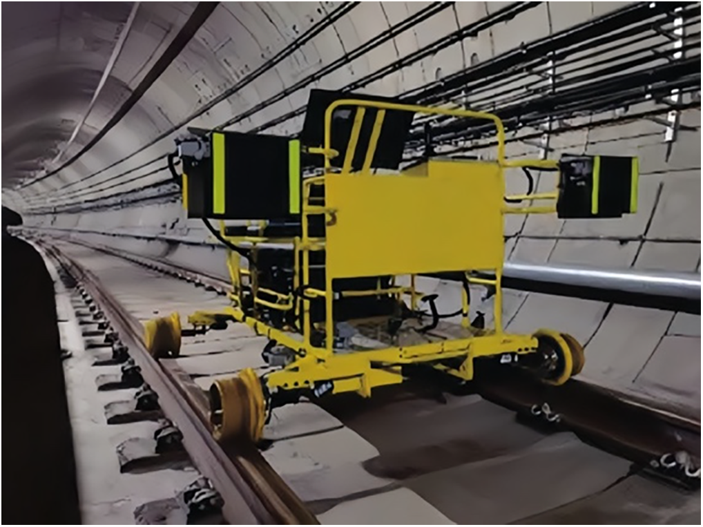
Figure 7: Railway information collection device

After a series of image processing steps, the images collected by the track inspection vehicle are cropped to 512 × 512 pixels. The open-source software LabelMe is used to annotate the ground truth information in the track images.

For the supervised model, we have a total of 1600 fastener images, consisting of 800 normal fastener images and 800 abnormal fastener images. To ensure a more robust evaluation of the model, we adopt k-fold cross-validation with k = 5, i.e., the 1600 images are divided into 5 subsets. In each round of cross-validation, 4 subsets (a total of 1280 images) are used for training, and 1 subset (320 images) is used for validation. After 5 rounds of training and validation, we calculate the average performance metrics to obtain a more comprehensive assessment of the model’s performance.

For the unsupervised model, we use 176 images for training. Among these, half of the images (88 images) are automatically turned into abnormal images through the model’s abnormal synthesis strategy. Similar to the supervised model, we also use 5-fold cross-validation. The 176 images are divided into 5 subsets. In each iteration, 4 subsets (around 140 images) are used for training, and 1 subset (around 35 images) is used for validation. We summarize the performance of the unsupervised model across the 5 rounds of cross-validation to understand its generalization ability.

The overall segmentation ratio of the training set to the test set is 7:3. In addition, we set aside 200 abnormal fastener images for model inference.

4.2 Training & Inference

4.2.1 Training Stage

We trained the reconstruction model and segmentation model together. The reconstruction model learns the entire distribution of a normal sample (y=0) by minimizing the following loss function:

ℒnoise=(1−y)(‖ϵts−ϵθ(xts)‖2+‖ϵtb−ϵθ(xts)‖2)2(7)

The segmentation model uses the commonalities and differences between x0 and x^0s to predict pixel-level anomaly scores that are as close as possible to the ground truth. Segmentation loss is defined as:

ℒmask=Smoothℒ1(M,M^)+γℒfocal(M,M^)(8)

where M is the truth mask of the input image, and M^ is the output of the segmentation model. Smoothℒ1 and ℒfocal were applied simultaneously to reduce oversensitivity to outliers and accurately segment difficult exception examples. γ∈R+ is the hyperparameter that controls the importance of ℒfocal. Therefore, the total loss of Diff-Fastener use for combined training is:

ℒtotal=ℒnoise+ℒmask(9)

4.2.2 Inference Stage

To achieve higher inference speed and reconstruction quality, we still use one-step norm-guided estimation in the inference stage. After the segmentation model predicts the pixel-level anomaly fraction M^, we take the average of the first K anomaly pixels in M^ as the image-level anomaly fraction. This inference method is hundreds of times faster while maintaining sampling quality.

4.3 Evaluation Metrics

To evaluate the anomaly detection performance of Diff-Fastener, we use the following metrics: Image AUROC, Pixel AUROC, precision rate and recall rate. Image AUROC is a metric used to evaluate the anomaly detection performance of the entire image and is the most widely used measure for anomaly assessment. It generates an ROC (Receiver Operating Characteristic) curve by calculating the true positive rate and false positive rate at different thresholds and computes the area under this curve. It provides a comprehensive performance evaluation for the entire image, making it suitable for scenarios that require consideration of overall anomalies in the image. Pixel AUROC is a metric used to assess the model’s anomaly detection performance at the pixel level. Unlike Image AUROC, Pixel AUROC focuses on the anomaly detection scores for each pixel and calculates the true positive rate and false positive rate at different thresholds. Pixel AUROC offers a detailed evaluation for each pixel, making it suitable for tasks that require precise localization of anomalous regions, such as image segmentation and fine-grained classification.

TPR=TPTP+FN(10)

FPR=FPFP+TN(11)

AUROC=∫01(TPR)d(FPR)(12)

Precision=TPTP+FP(13)

Recall=TPTP+FN(14)

AUPRO=∫01Precision(Recall)d(Recall)(15)

Note: TP stands for True Positive, FP for False Positive, TN for True Negative, FN for False Negative, TPR for True Positive Rate, and FPR for False Positive Rate.

4.4 Experimental Setup

Train and test Diff-Fastener on this dataset. The model adjusts all image inputs in the dataset to a resolution of 256 × 256, with the base channel set to 128, and the attention resolution set at 32, 16, and 8. The number of attention heads is set to 4. Set the number of epochs to 1500 and the batch size to 4, which includes 2 batches of normal samples and 2 batches of abnormal samples synthesized online through the anomaly synthesis strategy. The model employs the Adam optimizer for optimization, with an initial learning rate of 10−4. The research shows that the noise scale t is set to 400 to get better recovery [18]. All experiments were conducted on a GeForce RTX 4090.

4.5 Experimental Results and Discussion

4.5.1 Result Visualization

Fig. 8 shows the visualization of detection results for various types of fastener anomalies. It can be observed that Diff-Fastener does not require prior learning of specific anomaly categories. By simply training with samples of healthy fastener images, it can detect various fastener anomalies and successfully repair them, while maintaining high image fidelity. Among them, the model performs best in detecting two types of anomalies: broken and missing fasteners. It indicates that scenarios where objects transition from absent to present are clearly more suitable for anomaly detection based on generative models.

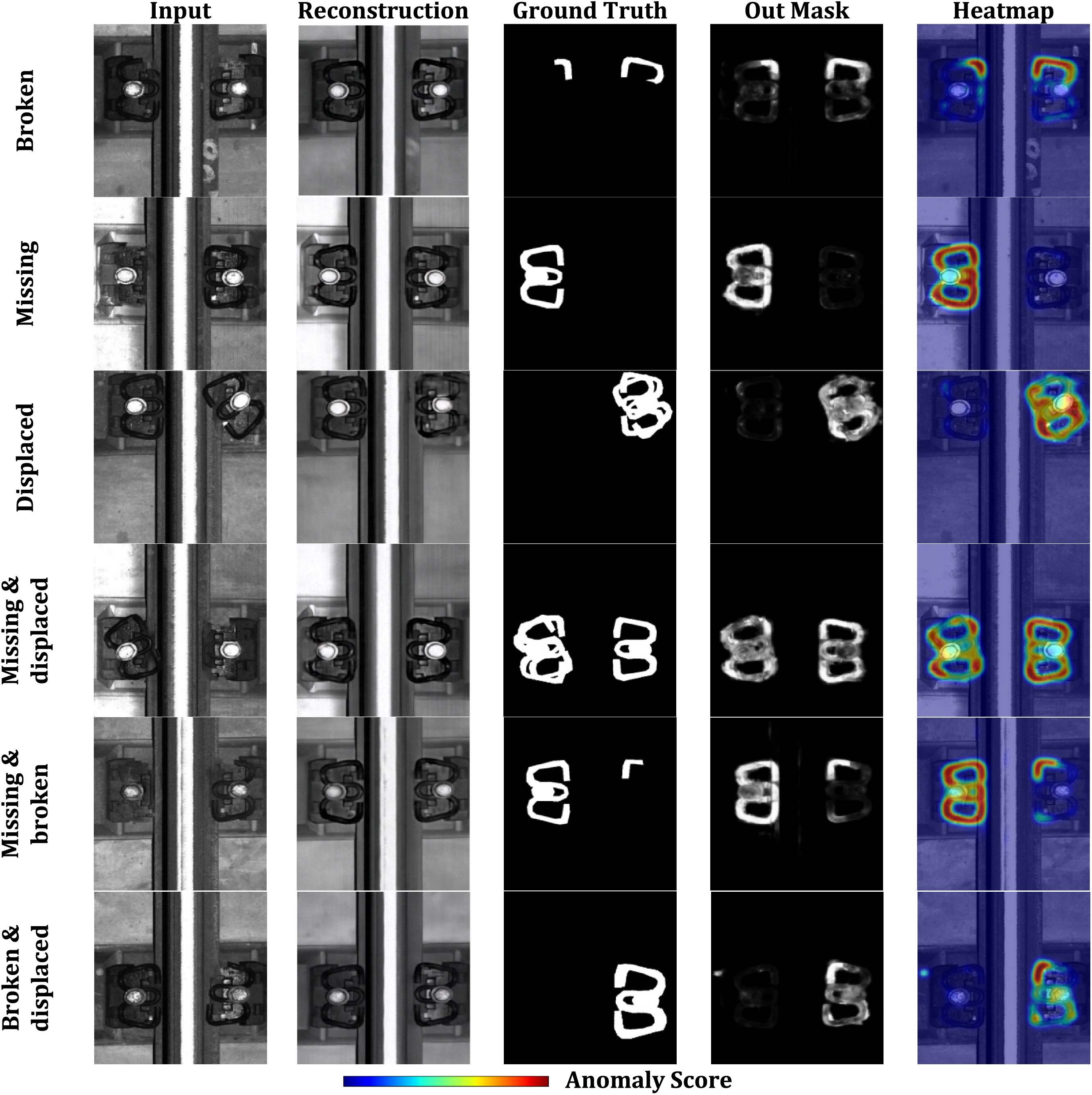
Figure 8: Visualization of anomalous fastener detection results

4.5.2 Comparative Experiment

By using cross-validation, we have obtained a more reliable assessment of the performance of both the supervised and unsupervised models. The average performance metrics from cross-validation provide a better understanding of the models’ generalization ability.

(1) Supervised models

This paper trains and tests the current advanced supervised detection model on the rail fastener dataset, and compares the results based on the recall rate and accuracy index at the label-level (i.e., at the whole image level). The comparison results are presented in Table 1, and the visualization of the comparison results can be seen in Fig. 9. Diff-Fastener learns fastener features by simply adding noise to and denoising healthy data, it can achieve approximately 99.9% accuracy rates and 99.9% recall rates in the label-level, that is, it can judge whether there is an anomaly in each fastener image almost perfectly. This result is of great significance, as it demonstrates the feasibility of the unsupervised detection model in the field of abnormal fastener detection.

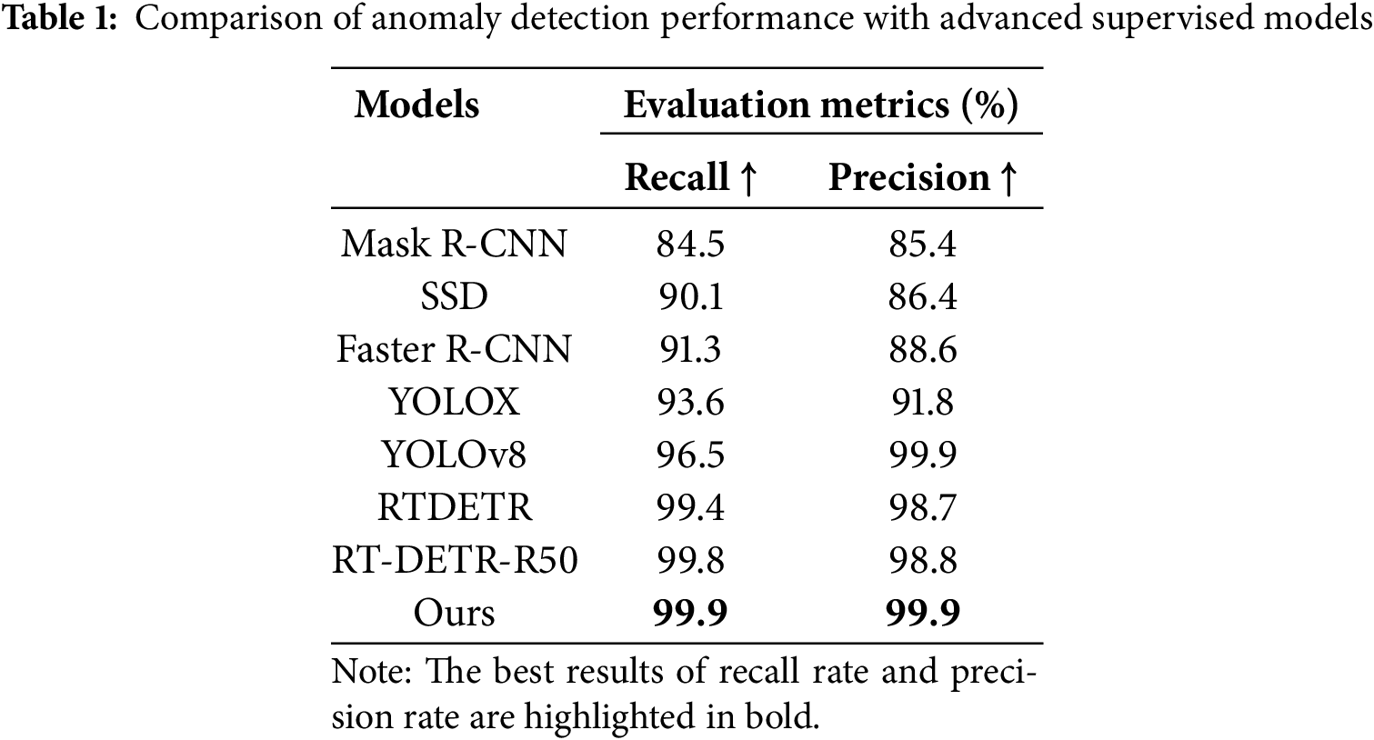
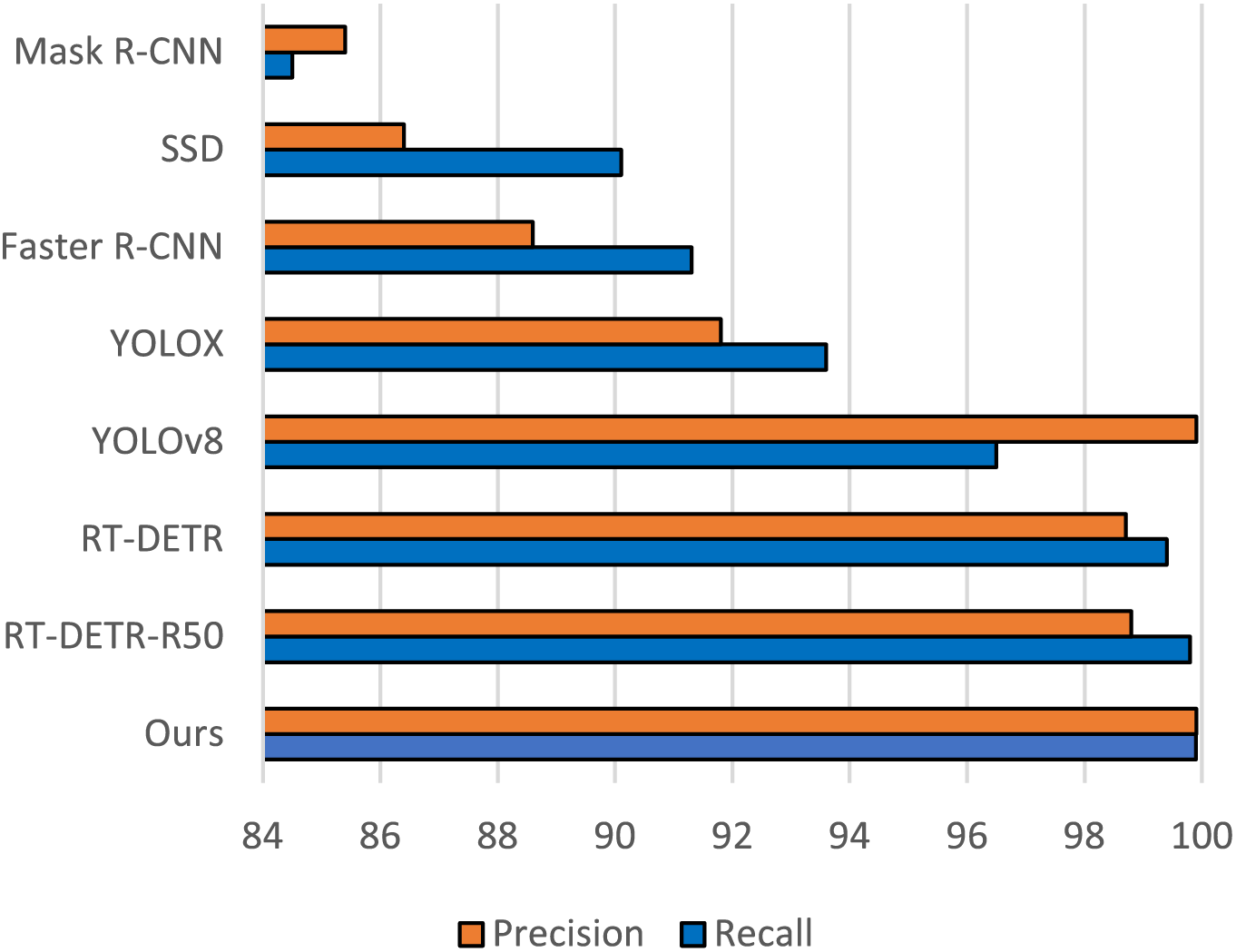
Figure 9: Bar chart comparing the label-level P&R performance of Diff-Fastener with advanced supervised detection models

(2) Unsupervised models

The MVTec [29] and VisA [30] datasets are essential benchmarks for anomaly detection. MVTec, with its 5000+ high-resolution images across 15 categories and pixel-precise anomaly annotations, is a gold standard for evaluating industrial inspection algorithms. VisA, offering 9621 normal and 1200 abnormal images in 12 categories, provides a new testbed for diverse industrial scenarios.

We compared the anomaly detection performance of Diff-Fastener with three feature embedding-based methods and three generative model-based methods; the results are presented in Table 2. The visualization of the comparison results can be seen in Fig. 10. The results show that for average Image AUROC, our model outperforms the feature embedding-based SOTA by 1.6% and the generative model-based SOTA by 0.3%. For average Pixel AUROC, our model outperforms the feature embedding-based SOTA by 2.9% and the generative model-based SOTA by 0.4%. The performance of Diff-Fastener is significantly better than previous models.

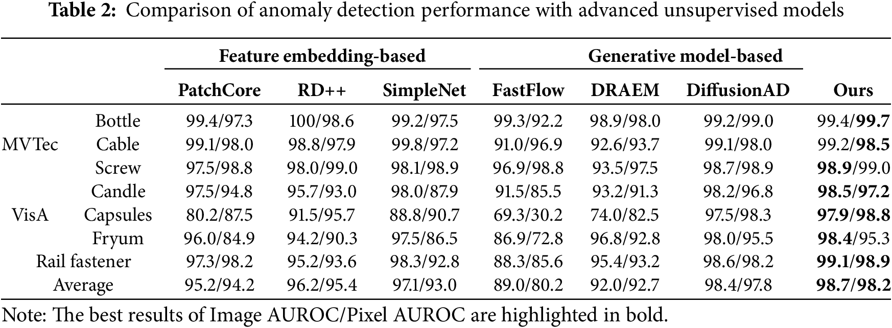
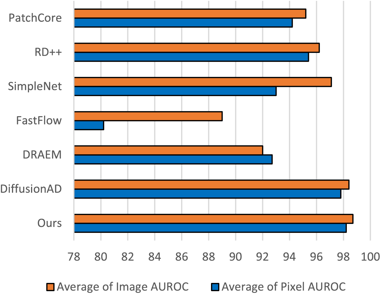
Figure 10: Bar chart comparing the average Image AUROC and Pixel AUROC with advanced unsupervised detection models

4.5.3 Ablation Study

Table 3 shows the results of the ablation study. From the first and second rows of the table, compared to traditional iterative denoising, the inference speed of One-Step denoising is greatly improved, approximately 320 times faster than before. In the third row, the use of the Norm-Guided paradigm enhances the model’s ability to preserve image details while effectively removing anomaly regions of varying sizes, achieving more accurate anomaly detection, with a slight decrease in speed. From the fourth to sixth rows, it is evident that the introduction of CBAM (Convolutional Block Attention Module) [31] and dilated convolutions [32] improves the model’s semantic awareness while maintaining relatively efficient speed. In addition, sparse skip has enhanced the network performance and detection efficiency. Ablation experiments have demonstrated the effectiveness of the above methods.

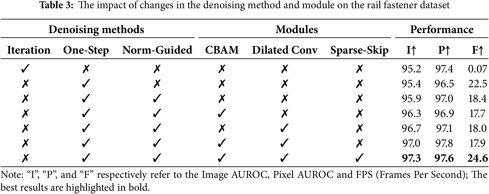
Fig. 11 shows the effects of the Norm-Guided paradigm and DACM. Fig. 11a–f represents several different anomalous samples. A indicates a diffusion model structure using only one-step denoising. The introduction of one-step denoising leads to a loss of detail in the reconstruction results, limiting adaptability to different types of anomalies. From the image, it can be seen that the reconstructed semantic edges of the fasteners are unclear, with some even experiencing spatial distortion, and the overall tone of the image appears unnatural. B represents a one-step denoising diffusion model after the introduction of the Norm-Guided paradigm, which allows for more refined reconstruction rather than simple rough recovery. Additionally, the model can effectively handle anomalies in varying-sized areas with two scales of noise, enhancing the model’s adaptability. However, there is still an issue of excessive image smoothing. After introducing DACM, the model can emphasize important features while suppressing less significant ones during the reconstruction process. It also captures a broader context in the feature extraction stage, further enhancing the model’s reconstruction capability. As shown in Fig. 11, our reconstructed images contain richer detail information and are more aligned with real-world situations.

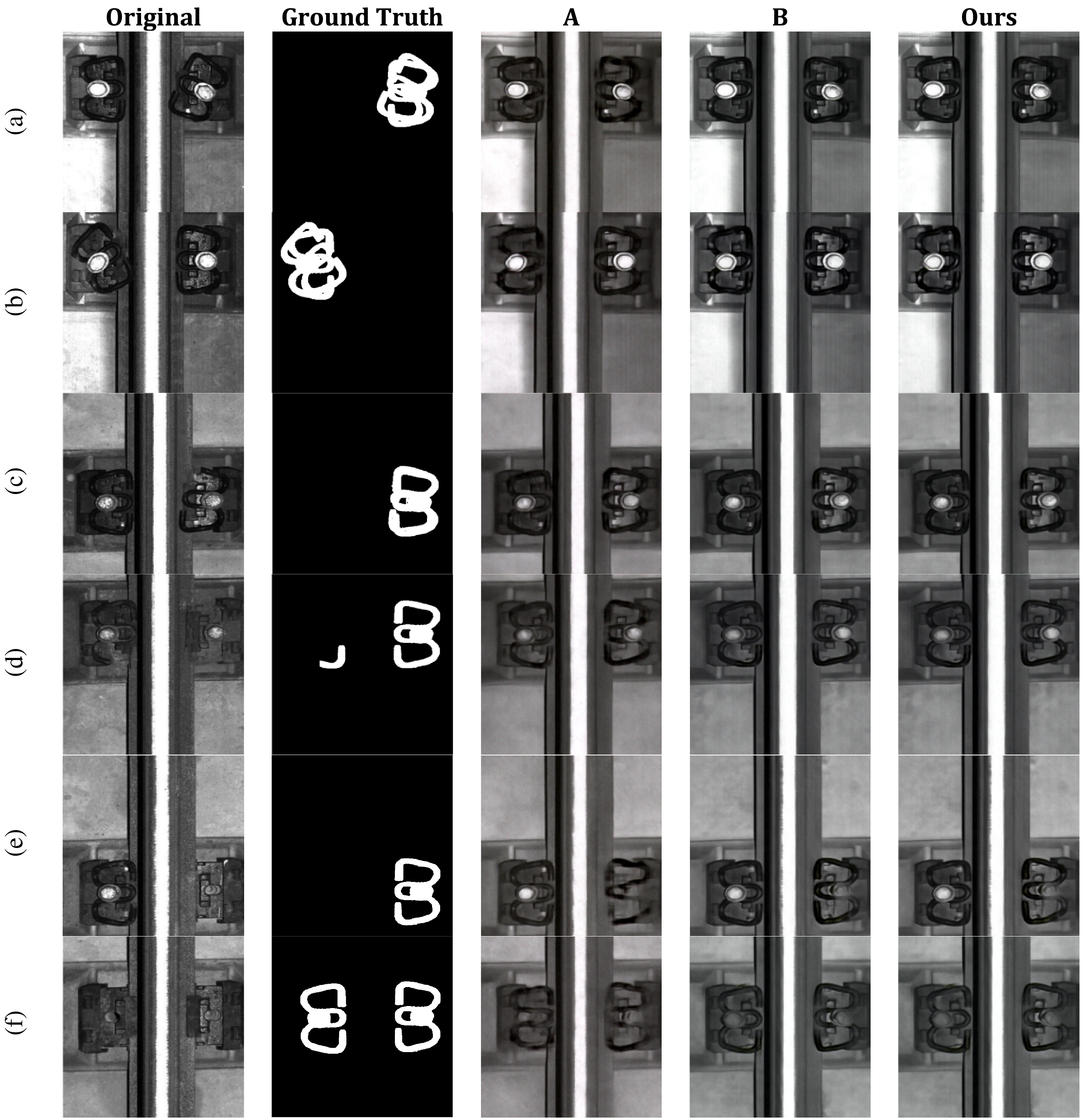
Figure 11: Ablations of norm-guided paradigm and CBAM & Dilated Convolution on rail fastener dataset

5  Conclusion

In this paper, we propose Diff-Fastener, a model that, for the first time, utilizes the generative ability of the diffusion model to detect abnormal fasteners. We employ one-step denoising to alleviate the inefficiency issues associated with traditional iterative denoising methods. The introduction of the Norm-Guided paradigm brings the model’s ability for finer reconstruction and better adaptability. DACM further improves the model’s feature selection capability, resulting in stronger accuracy in complex scenes. The high efficiency of sparse skip has enhanced the scalability of the model. Experiments have demonstrated that this model has strong effectiveness and practicality, and it possesses practical application value in actual railway engineering scenarios. Meanwhile, we hope this work can reignite interest in denoising-based railway fault diagnosis methods within the context of current research in unsupervised learning.

Acknowledgement: Not applicable.

Funding Statement: This research was funded by the National Natural Science Foundation of China, grant number 52272385 and 52475085.

Author Contributions: The authors confirm contribution to the paper as follows: Conceptualization, Peng Sun; methodology, Peng Sun; software, Peng Sun; validation, Peng Sun and Quanyu Long; formal analysis, Peng Sun; investigation, Peng Sun; resources, Dechen Yao and Jianwei Yang; data curation, Peng Sun; writing—original draft preparation, Peng Sun; writing—review and editing, Peng Sun and Jianwei Yang; visualization, Peng Sun; supervision, Dechen Yao and Jianwei Yang; project administration, Dechen Yao and Jianwei Yang; funding acquisition, Dechen Yao and Jianwei Yang. All authors reviewed the results and approved the final version of the manuscript.

Availability of Data and Materials: Data not available due to ethical restrictions. Due to the nature of this research, participants of this study did not agree for their data to be shared publicly, so supporting data is not available.

Ethics Approval: Not applicable.

Conflicts of Interest: The authors declare no conflicts of interest to report regarding the present study.

References

1. Min Y, Jing Q, Li Y. Method for rail surface defect detection based on neural network architecture search. Meas Sci Technol. 2024;36(1):016027. doi:10.1088/1361-6501/ad9048. [Google Scholar] [CrossRef]

2. Roth K, Pemula L, Zepeda J, Schölkopf B, Brox T, Gehler P. Towards total recall in industrial anomaly detection. arXiv:2106.08265v2. 2021. [Google Scholar]

3. Tien TD, Nguyen AT, Tran NH, Huy TD, Duong STM, Nguyen CDT, et al. Revisiting reverse distillation for anomaly detection. In: Proceedings of the 2023 IEEE/CVF Conference on Computer Vision and Pattern Recognition (CVPR); 2023 Jun 17–24; Vancouver, BC, Canada. doi:10.1109/CVPR52729.2023.02348. [Google Scholar] [CrossRef]

4. Liu Z, Zhou Y, Xu Y, Wang Z. SimpleNet: a simple network for image anomaly detection and localization. arXiv:2303.15140v2. 2023. [Google Scholar]

5. Yu J, Zheng Y, Wang X, Li W, Wu Y, Zhao R, et al. FastFlow: unsupervised anomaly detection and localization via 2D normalizing flows. arXiv:2111.07677v2. 2021. [Google Scholar]

6. Zavrtanik V, Kristan M, Skočaj D. DRAEM—a discriminatively trained reconstruction embedding for surface anomaly detection. arXiv:2108.07610v2. 2021. [Google Scholar]

7. Wei Y. Review: recent advances for the diffusion model. J Phys Conf Ser. 2024;2711(1):012005. doi:10.1088/1742-6596/2711/1/012005. [Google Scholar] [CrossRef]

8. Bhosale A, Mukherjee S, Banerjee B, Cuzzolin F. Anomaly detection using diffusion-based methods. arXiv:2412.07539. 2024. [Google Scholar]

9. Livernoche V, Jain V, Hezaveh Y, Ravanbakhsh S. On diffusion modeling for anomaly detection. arXiv:2305.18593. 2025. [Google Scholar]

10. Ahsan MM, Raman S, Liu Y, Siddique Z. A comprehensive survey on diffusion models and their applications. arXiv:2408.10207. 2024. [Google Scholar]

11. Ho J, Jain A, Abbeel P. Denoising diffusion probabilistic models. arXiv:2006.11239. 2020. [Google Scholar]

12. Mousakhan A, Brox T, Tayyub J. Anomaly detection with conditioned denoising diffusion models. arXiv:2305.15956. 2023. [Google Scholar]

13. Wolleb J, Bieder F, Sandkühler R, Cattin PC. Diffusion models for medical anomaly detection. arXiv:2203.04306. 2022. [Google Scholar]

14. Pinaya WHL, Graham MS, Gray R, Costa PFD, Tudosiu PD, Wright P, et al. Fast unsupervised brain anomaly detection and segmentation with diffusion models. arXiv:2206.03461. 2022. [Google Scholar]

15. Wyatt J, Leach A, Schmon SM, Willcocks CG. AnoDDPM: anomaly detection with denoising diffusion probabilistic models using simplex noise. In: Proceedings of the 2022 IEEE/CVF Conference on Computer Vision and Pattern Recognition Workshops (CVPRW); 2022 Jun 19–20; New Orleans, LA, USA. doi:10.1109/CVPRW56347.2022.00080. [Google Scholar] [CrossRef]

16. He H, Zhang J, Chen H, Chen X, Li Z, Chen X, et al. DiAD: a diffusion-based framework for multi-class anomaly detection. arXiv:2312.06607. 2023. [Google Scholar]

17. Song J, Park D, Baek K, Lee S, Choi J, Kim E, et al. DefectFill: realistic defect generation with inpainting diffusion model for visual inspection. arXiv:2503.13985v1. 2025. [Google Scholar]

18. Zhang H, Wang Z, Wu Z, Jiang YG. DiffusionAD: norm-guided one-step denoising diffusion for anomaly detection. arXiv:2303.08730. 2023. [Google Scholar]

19. Rombach R, Blattmann A, Lorenz D, Esser P, Ommer B. High-resolution image synthesis with latent diffusion models. arXiv:2112.10752. 2022. [Google Scholar]

20. Song J, Meng C, Ermon S. Denoising diffusion implicit models. arXiv:2010.02502. 2022. [Google Scholar]

21. He K, Zhang X, Ren S, Sun J. Deep residual learning for image recognition. arXiv:1512.03385. 2015. [Google Scholar]

22. Salimans T, Karpathy A, Chen X, Kingma DP. PixelCNN++: improving the PixelCNN with discretized logistic mixture likelihood and other modifications. arXiv:1701.05517v1. 2017. [Google Scholar]

23. Vaswani A, Shazeer N, Parmar N, Uszkoreit J, Jones L, Gomez AN, et al. Attention is all you need. arXiv:1706.03762. 2023. [Google Scholar]

24. Long C, Tan C, Li Q, Tan H, Duan L. Industrial CT image reconstruction for faster scanning through U-Net++ with hybrid attention and loss function. Nondestruct Test Eval. 2024;39(8):2646–65. doi:10.1080/10589759.2024.2305329. [Google Scholar] [CrossRef]

25. Shang F, Cai D, Sun B, Han Y, Yang M, Zhan C. Research on weld seam feature extraction and defect identi-fication technology. Nondestruct Test Eval. 2024. doi:10.1080/10589759.2024.2405062. [Google Scholar] [CrossRef]

26. Wang Y, Dong M, Shen J, Lin Y, Pantic M. Dilated convolutions with lateral inhibitions for semantic image segmentation. arXiv:2006.03708. 2022. [Google Scholar]

27. Yang M, Wu P, Liu J, Feng H. MemSeg: a semi-supervised method for image surface defect detection using differences and commonalities. arXiv:2205.00908. 2022. [Google Scholar]

28. Zhang H, Wu Z, Wang Z, Chen Z, Jiang YG. Prototypical residual networks for anomaly detection and localization. arXiv:2212.02031. 2023. [Google Scholar]

29. Bergmann P, Batzner K, Fauser M, Sattlegger D, Steger C. The MVTec anomaly detection dataset: a comprehensive real-world dataset for unsupervised anomaly detection. Int J Comput Vis. 2021;129(4):1038–59. doi:10.1007/s11263-020-01400-4. [Google Scholar] [CrossRef]

30. Zou Y, Jeong J, Pemula L, Zhang D, Dabeer O. SPot-the-difference self-supervised pre-training for anomaly detection and segmentation. arXiv:2207.14315. 2022. [Google Scholar]

31. Woo S, Park J, Lee JY, Kweon IS. CBAM: convolutional block attention module. arXiv:1807.06521. 2018. [Google Scholar]

32. Yu F, Koltun V. Multi-scale context aggregation by dilated convolutions. arXiv:1511.07122. 2016. [Google Scholar]