The Advanced Structural Health Monitoring by Non-Destructive Self-Powered Wireless Lightweight Sensor

1  Introduction

Bridge resilience refers to a bridge’s ability to withstand and recover from disruptions, ensuring its continued functionality and safety. This involves considering various factors like natural hazards, accidental actions, and the bridge’s ability to be repaired quickly after damage. In essence, bridge resilience is not just about structural strength, but also about the ability to adapt, recover, and continue to serve its purpose in the face of various challenges [1–3].

Sensors play a vital role in monitoring the health of bridge structures. Strain gauges, vibration sensors and other equipment can sense and collect data on structural changes in bridges, roads and other transportation infrastructure in real time, accurately capturing structural deformation, strength, displacement, etc. Key information helps maintenance personnel understand the status and health of facilities in real time.

As a product of the innovative development of communication technology, wireless sensors are increasingly becoming the key to sensor research and application. Its development history can be traced back to the late 1990s. Since the landmark discussion of “sensors moving towards the wireless era”, sensor technology has evolved from general sensors to smart sensors and then to wireless sensors. Wireless sensors not only integrate data acquisition and processing functions, but also realize real-time information exchange and control through wireless functional modules, forming a system that integrates data acquisition, processing, exchange and control [4–6].

As things evolve, wireless sensor modules are really stepping up as a key player in data collection and communication within the wireless tech field. These networks blend sensor technology with embedded computing, modern networking, and wireless communication, along with distributed information processing. That’s why they’re such a hot topic in research these days [7–9].

Looking back on the development of bridge structure health monitoring, the core goal of structural monitoring is to evaluate the response of the structure to extreme events, which requires sensors to be highly adaptable.

At the same time, the existing self-generation technology is not yet mature, and the power generation mode needs to be further optimized and improved to meet the long-term stable operation requirements of wireless sensor nodes. The widespread application of low power consumption has promoted its development in the direction of wireless communication networking, that is, to form a dynamic and adaptive wireless sensor network through a self-organizing network. On the basis of ensuring network reliability, the development of wireless sensor modules should be committed to achieving the goals of low power consumption and high performance [10–13].

To further enhance the comprehensiveness and academic, the several recent and relevant studies in the field of turboelectric nanogenerators that consider the basic of the SPWL Technology. These studies offer valuable insights into material selection, device architecture, and multifunctional applications of Lightweight sensors [14–17].

Building on the SPWL sensors design concept mentioned earlier, we’ve come up with a design method for a tunnel monitoring model that includes input/output, and estimation components [18–20].

1.   The monitoring system for tracking the tunnel’s input load will be set up wirelessly. This system needs to follow the SPWL sensors design principles—this means we have to think about what to monitor, how to lay out the measuring points, and what equipment to choose. When choosing what to monitor, we should refer to relevant standards for tunnel operations and maintenance, along with the specific needs of the project. This will help us focus on long-term monitoring of critical areas. For the measuring point layout, we’ll pick key sections that matter most and monitor their parameters wisely. As for the equipment, it should be durable, energy-efficient, and accurate, in line with the SPWL sensors concept.

2.   The output system of tunnel monitoring is all about processing the monitoring data, filtering out any weird readings, and applying a scoring calculation formula from the standards to determine the structural health of the tunnel.

3.   In terms of evaluating the tunnel monitoring system, we’ll use the technical condition scores defined in the standards to assess the data output. This helps us evaluate the stability of the tunnel and decide on any necessary maintenance actions.

In short, the SPWL sensor design approach for the monitoring model has three key elements: input/output, and valuation. We start by gathering real-time data on the structure, process it, and then produce a score that reflects the tunnel’s technical condition. By comparing these scores, we can assess the tunnel’s stability.

However, although domestic and foreign scholars have made significant progress in wireless sensor network networking technology, the research on the adaptability of lightweight monitoring and the integrated exploration of sensor edge computing capabilities are still insufficient. This paper focuses on creating lightweight, self-powered wireless sensors designed for complete, real-time monitoring of critical infrastructure like tunnels, bridges, and slopes. These advancements aim to support smart infrastructure that can comprehensively assess important structures, which is crucial for enhancing the safety and efficiency of highway operations.

2  Methodology

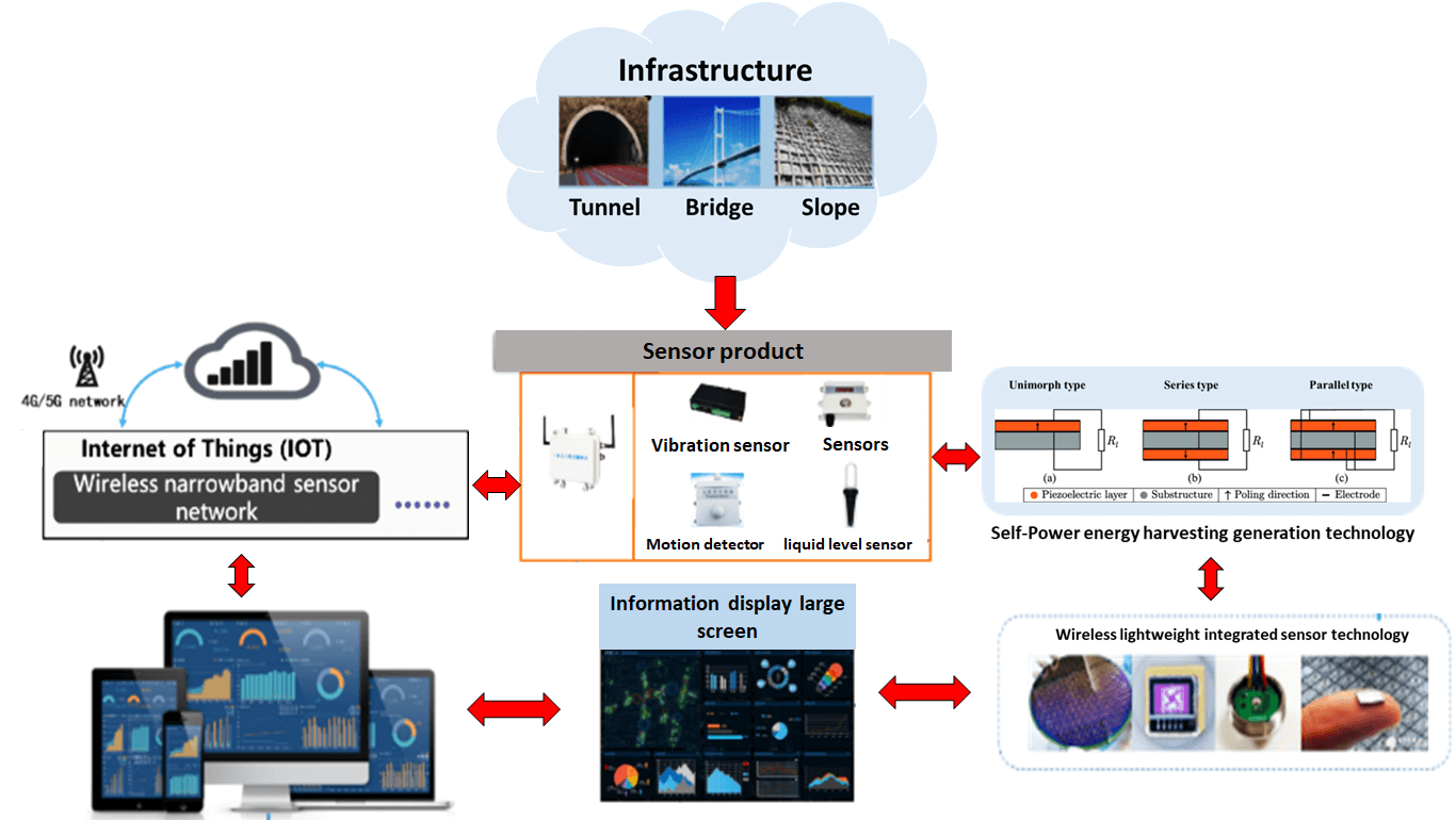
To sum it up, sensors gather essential data that help keep an eye on the structural integrity of things like roads, tunnels, and bridges, making possible monitoring to be lightweight. With the development of SPWL sensors, we can quickly and efficiently set them up in tricky bridge and tunnel situations, and they cover a broad tracking range. This approach helps save resources and makes management easier. Plus, SPWL sensors are built to last, extending their lifespan and durability for ongoing monitoring. They offer real-time data analysis, give early warnings, and support maintenance decisions, fulfilling the long-term monitoring needs for infrastructure. You can check out the schematic diagram based on SPWL sensors in Fig. 1.

Figure 1: Schematic diagram of lightweight infrastructure monitoring system framework

The low-power wireless sensor system is made up of a few key parts: a module for generating external power, a power management module, one for collecting and processing physical data, and a module for wireless communication. The power generation part primarily takes kinetic, potential, and light energy from the road and converts it into electricity through different methods. Depending on the setting, we choose various techniques. For example, we might use ceramic piezoelectric generators, wind power, or solar panels, either separately or together, depending on what’s needed. The power management part carefully handles how energy storage devices charge and discharge to keep the power usage low while making sure everything runs smoothly. As for the data collection and processing module, it detects and gathers information from the objects being monitored, converting it into digital signals. Finally, the wireless communication module sends these signals to a gateway or base station, as shown in Fig. 2.

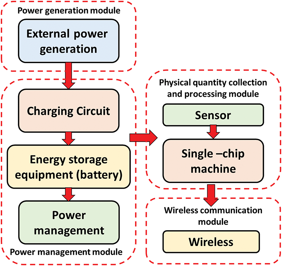
Figure 2: Wireless low power sensor module

2.1 Key Technology List

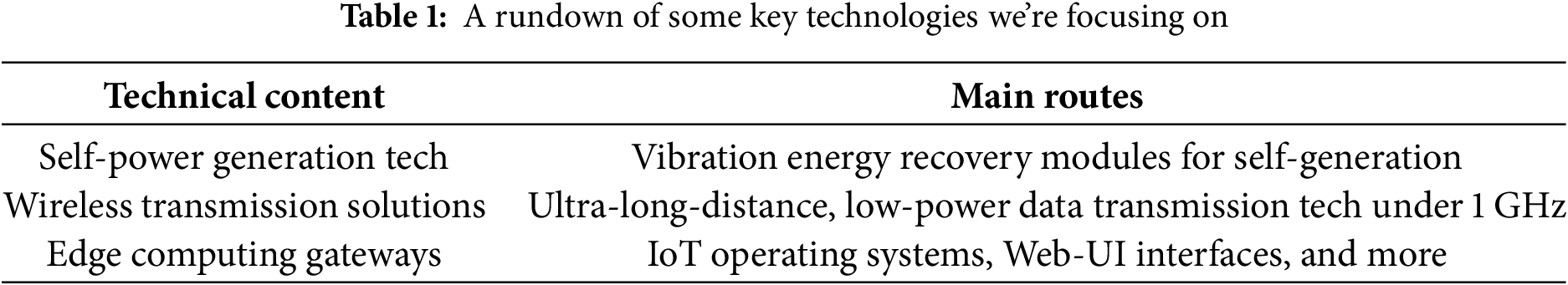
This paper focuses on some important technologies, like the self-generation tech for recovering vibration energy, wireless transmission, and edge computing gateways (check out Table 1 for more details).

2.2 Lightweight Technology

Lightweight tech for monitoring traffic infrastructure comes with some key features: it uses low-power sensors, has a long lifespan, is relatively compact, and is easy to implement. Thanks to these low-energy wireless sensors, wiring during construction is straightforward and costs are kept low. This setup allows for quick deployment, efficient networking, and effective data processing. Here’s a breakdown of how it works:

This lightweight technology for keeping tabs on traffic systems has some great features. It runs on low-power sensors, lasts a long time, is pretty compact, and is simple to set up. Because of these energy-efficient wireless sensors, you can avoid a lot of complicated wiring during construction, which helps keep costs down. This setup means you can deploy everything quickly, network efficiently, and process data effectively. Here’s a closer look at how it all comes together:

Information Transmission: Each sensor features its own wireless transmission capability. In different traffic scenarios, it can send monitoring data back to the main system in real-time without needing a Dedicated Terminal Unit (DTU), making the information transfer much easier.

Energy Consumption: These sensors are designed for low energy use and have a sleep mode. Their sleep current stays around microamps, so they don’t eat up much power at all.

Self-Generation: The sensors have a built-in energy collection system that allows them to recharge themselves over time, which is pretty handy.

Easy Implementation: Since we’re using battery-operated low-power wireless sensors, there’s no need for complicated wiring layouts. The setup costs are low, making it simple and convenient.

Take a look at Fig. 3 for an example of one of these lightweight, low-power wireless sensors.

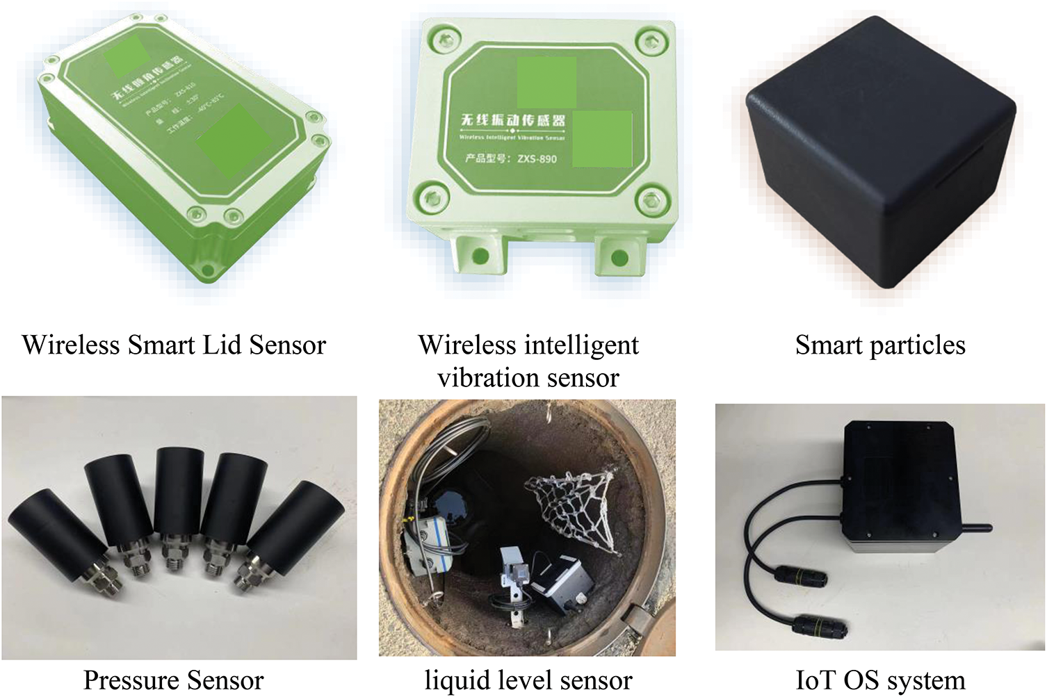
Figure 3: Illustration of a lightweight self-generating sensor device

2.3 Self-Power Generation Technology

Taking into account the overall costs and how the materials perform, this work aims to utilize piezoelectric transducer (PZT) ceramic array modules for generating electricity. Right now, PZT ceramics are the best option available for converting mechanical energy into electrical energy. They can produce various voltages and currents depending on whether they’re connected in parallel or series, as illustrated in Fig. 4.

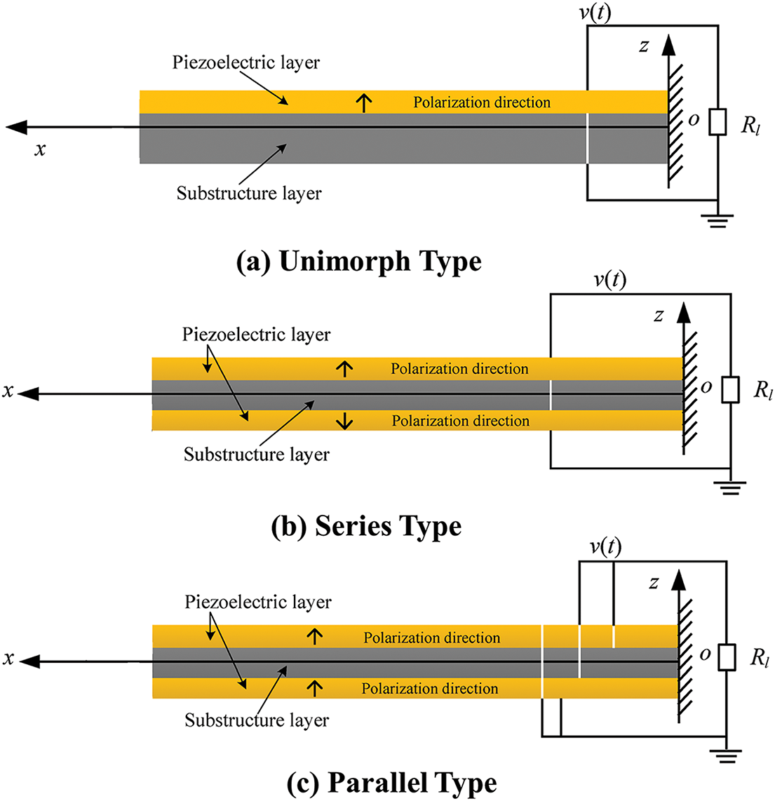
Figure 4: A diagram showing how power is generated using piezoelectric ceramics

For the piezoelectric elements we’ve discussed, we’ve decided to use single-sided and full-coverage protection. When the piezoelectric element is embedded in asphalt concrete, it’s important that the protective material around the piezoelectric ceramic can absorb some of the impact. This helps to cushion the effect of the force on the element. Polyvinyl chloride hard plastic and elastic rubber work best for protecting piezoelectric elements in power generation roads, as illustrated in Fig. 5.

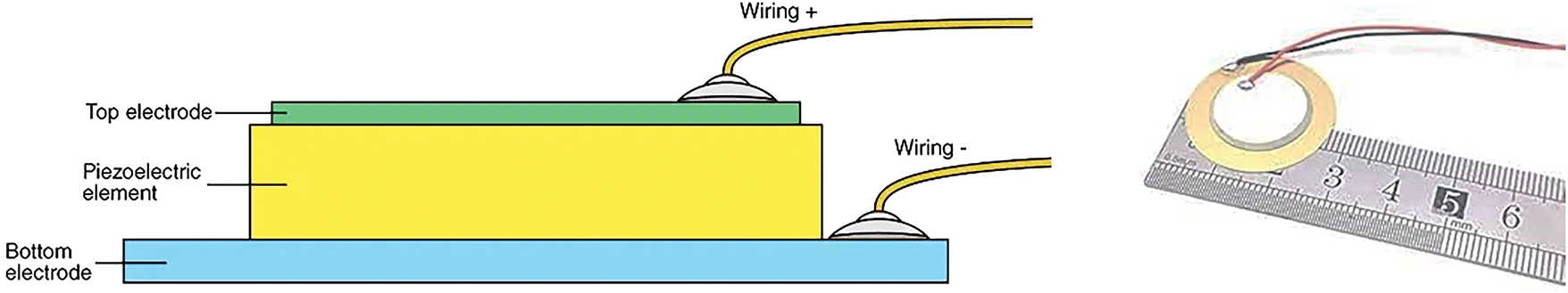
Figure 5: The piezoelectric ceramic power generation structure

The self-generating sensors used on the road are based on the energy harvesting technology of piezoelectric ceramics, which can convert the mechanical energy generated during road driving into electrical energy. This technology uses the characteristics of piezoelectric ceramic materials to generate electric charges when subjected to pressure or stress, thereby generating electricity adapted from [2]. By installing these materials in areas with high traffic flow, road power generation devices can collect energy without affecting the normal passage of vehicles and pedestrians.

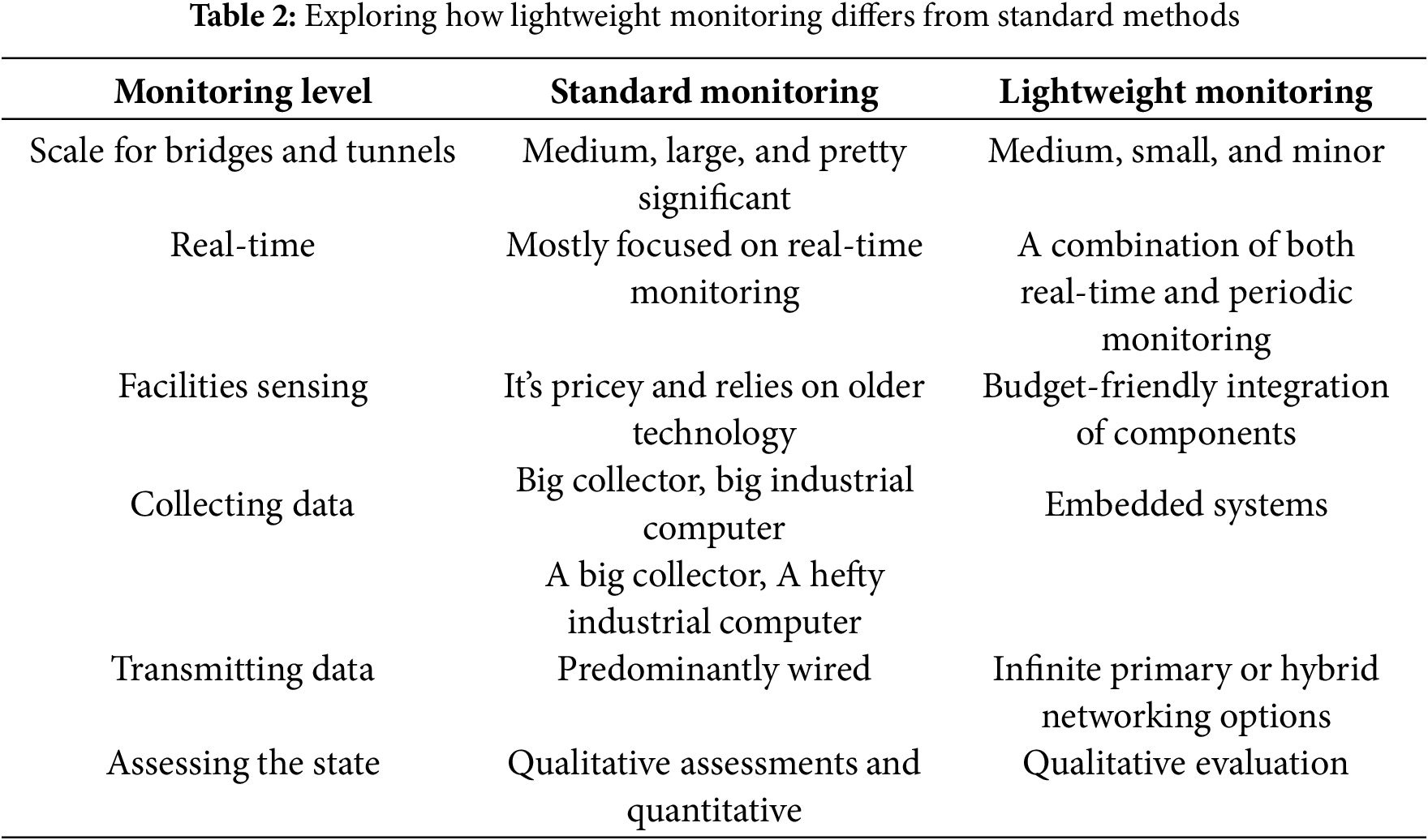
2.4 A Look at Lightweight vs. Standard Sensor Monitoring

In transportation infrastructure, like bridges and tunnels, we often use various sensors, including strain gauges, displacement gauges, thermometers, hygrometers, water level gauges, inclinometers, and accelerometers, depending on what physical quantity we’re measuring. You can see a comparison of lightweight vs standard monitoring methods in Table 2 below.

2.5 Specifications for Lightweight Sensor Technology

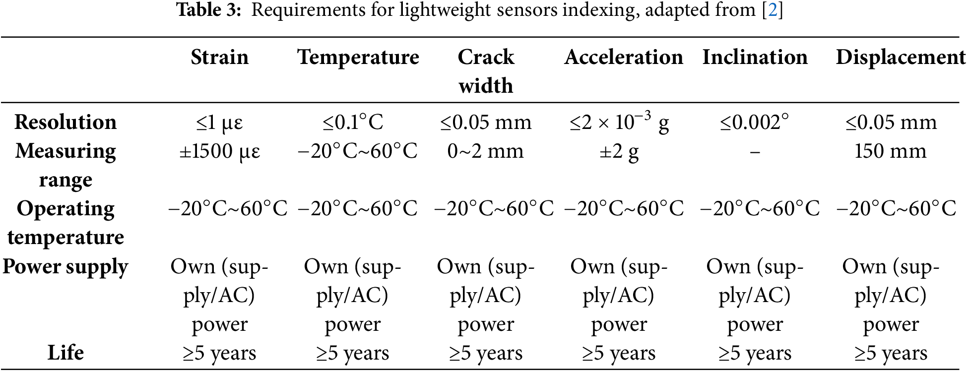
Check out Table 3 for the technical specs needed for lightweight sensors.

2.6 Lightweight Sensor Integrated Design

Traditional sensors tend to be bulky and heavy, thanks to factors like their power supply and communication needs. This often leads to a limited battery life, which means they have to be replaced frequently. The waste that this generates and the resulting environmental impact can’t be overlooked.

On the other hand, energy capture devices that use ceramic piezoelectric materials come with several benefits. They have a straightforward design, don’t generate heat, are free from electromagnetic interference, and don’t cause pollution. Plus, they lend themselves well to miniaturization and integration, making them ideal for low-energy products. This has garnered quite a bit of attention. By designing an integrated platform that combines the energy capture, communication, and sensing functions of sensors, we can enjoy advantages like a simple structure, no heat generation, a lack of electromagnetic interference, and ease of processing and manufacturing. This approach is really important for cutting down on power consumption, enhancing communication performance, reducing size, and simplifying installation, as illustrated in Fig. 6.

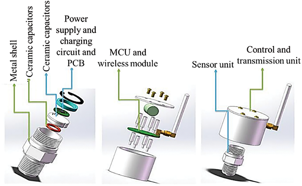
Figure 6: Schematic diagram of integrated sensor structure

3  Current Sensor Application

This paper looks into a lightweight monitoring technology, using the Jiefanghe Bridge on the Hangjinqu Expressway as a case study. It blends actual engineering practices with the necessary specifications, picking appropriate lightweight monitoring solutions based on the identified issues. Data from wireless vibration and temperature sensors is first sent to a wireless gateway, which then connects to a switch to upload data in real-time. As for the construction plan, it involves mounting the wireless gateway on the bridge column wall, drawing power from the bridge’s lighting mains to keep the wireless gateway running, as illustrated in Fig. 7.

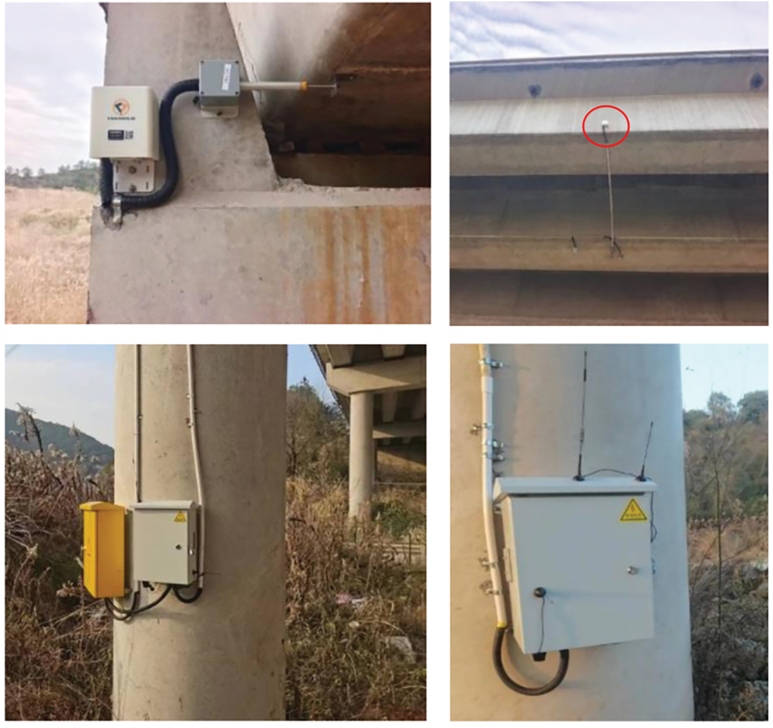
Figure 7: Equipment installation and deployment

By putting in some high-tech sensors and automated equipment, along with setting clear limits, we can keep track of important signals about the bridge’s structural health—things like stress, displacement, and deflection. This info is evaluated, categorized, and recorded in real-time. If something goes wrong, we can send out alerts through different channels like websites, emails, or text messages to inform the right people right away.

Plus, it helps us monitor environmental factors, the bridge’s condition, and any issues it might have. We gather data from various sources, analyze it, and then assess the overall safety and functionality of the bridge and its main parts. This way, we can keep a close eye on how the bridge is performing and spot any potential problems early on. By warning everyone at the first signs of trouble, we can significantly reduce the risk of serious accidents. The monitoring system covers several aspects including temperature, humidity, vibration, deformation, displacement, and strain.

4  Results and Discussions

We used a lightweight sensor monitoring system on the Jiefang River Bridge and got some interesting analysis results. This paper looks at the structural vibration signals using the empirical mode decomposition (EMD) method, especially how the intrinsic mode function (IMF) components change over time, measured in seconds. The IMF components are crucial for analyzing vibration signals since they can pick up different frequency elements in the signal, which helps us monitor the overall health of the structure.

In our study, the baseline measurements show the vibration traits of the structure when it’s functioning normally, acting as a reference point. When we dive into the measured values of the nine IMF components over time, as shown in Fig. 8, we noticed that some of the IMFs showed more significant fluctuations, particularly the IMF9 component. These fluctuations could point to changes in the structure’s condition, potentially indicating damage or shifts in its dynamic characteristics.

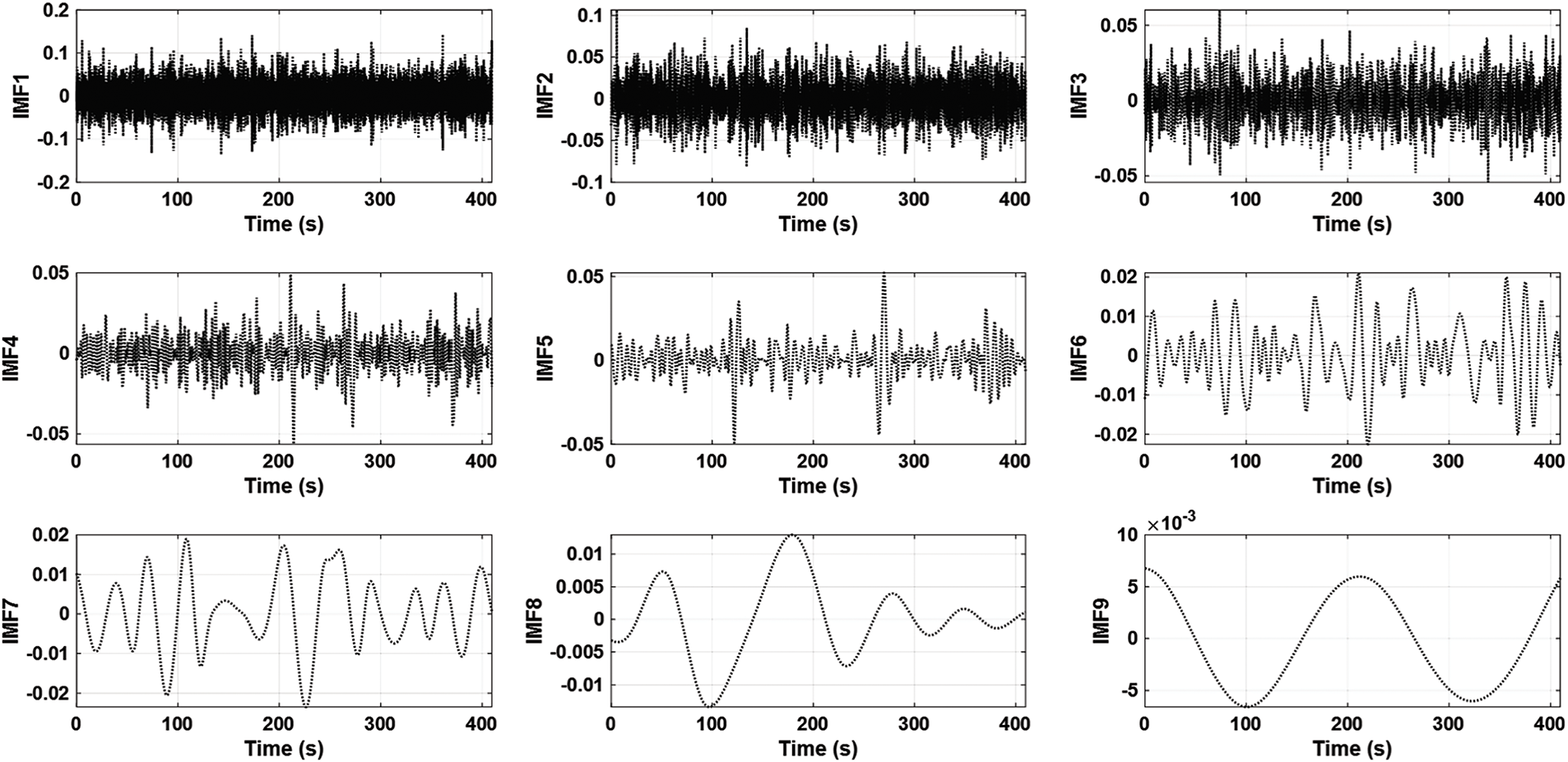
Figure 8: The intrinsic mode function (IMF) component over time of the baseline vibration measurement for the bridge baseline condition

It’s interesting to note that the second plot in Fig. 8 shows some pretty big fluctuations, particularly in the lower-order IMF components like IMF9. This could mean there are higher vibration levels, possibly due to some damage or issues with the structure’s integrity. On the flip side, Fig. 9 presents a more uniform vibration pattern, while the earlier plot indicates a lot more variability. In the realm of structural health monitoring, these kinds of changes in patterns or amplitudes are typically seen as signs that something’s off with the structure’s condition.

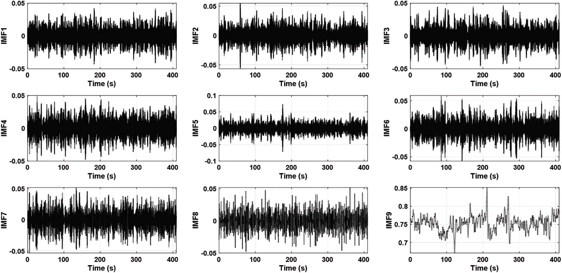
Figure 9: The intrinsic mode function (IMF) component over time of vibration measurements for the bridge current condition

When we looked at the differences in the IMF components between the baseline and the current data, we noticed some significant disparities. This might point to a shift in the bridge’s health. Still, to be really sure about the structure’s condition, engineers usually need to dive deeper into more extensive data. This could involve longer monitoring periods with additional sensors to back up any insights gained from the IMF comparison.

Figs. 10 and 11 illustrate the frequency patterns of Intrinsic Mode Functions (IMFs) obtained from the bridge’s vibration data, analyzed with the Hilbert-Huang Transform (HHT). This kind of analysis is essential for monitoring the bridge’s structural health, as it helps identify changes in its characteristics over time that might hint at damage or wear. In Fig. 10, representing the baseline condition, the frequencies appear to remain fairly stable, with only minimal fluctuations. This stability implies there weren’t any significant structural changes or damages at that point. Some of the lower frequency content in certain IMFs might be linked to the bridge’s fundamental structural frequencies, and their consistency is a good sign of overall structural health. On the other hand, Fig. 11 compares the current condition of the bridge to the baseline and reveals notable differences in the frequency content, showing more variations over time. The fluctuations seen could indicate potential structural changes or damage. For instance, if frequencies increase, it might signal a loss of mass or stiffness in some components of the bridge. The lower IMFs, which typically capture the main structural frequencies, appear to be more variable now, raising concerns from a structural health monitoring standpoint. Plus, the range of frequencies in the current state seems to have shifted or expanded compared to the baseline, suggesting that new vibration modes are being activated due to structural changes. Additionally, the current condition plots indicate possible anomalies or sudden shifts in frequency, particularly at specific time points, which might relate to events or defects impacting the bridge. By comparing Figs. 10 and 11, engineers can track changes in the bridge’s structural behavior over time. Analyzing the differences in frequency content between the baseline and current conditions can help diagnose potential damage or inform maintenance decisions. It’s also worth noting that while some variability is normal due to environmental factors like temperature and wind, any significant deviations from the baseline could signal structural problems that need attention.

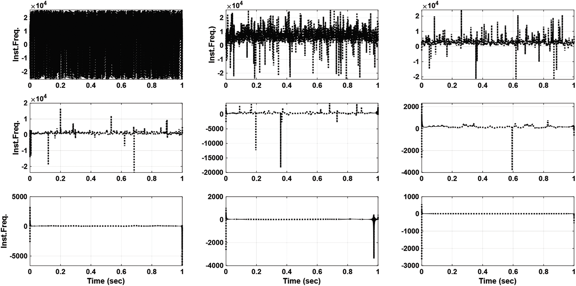
Figure 10: The instantaneous frequency of vibration measurement for the bridge baseline condition

Figure 11: The instantaneous frequency of vibration measurement for the bridge current condition

Fig. 12a illustrates the cumulative energy across intrinsic mode functions (IMFs) over a specified time frame. The X-axis represents the timeline from “2024-01-25” to “2024-02-29,” marking the period during which we observe energy changes in the IMFs. Meanwhile, the Y-axis showcases the cumulative energy of these IMFs, highlighting how their total energy fluctuates over time.

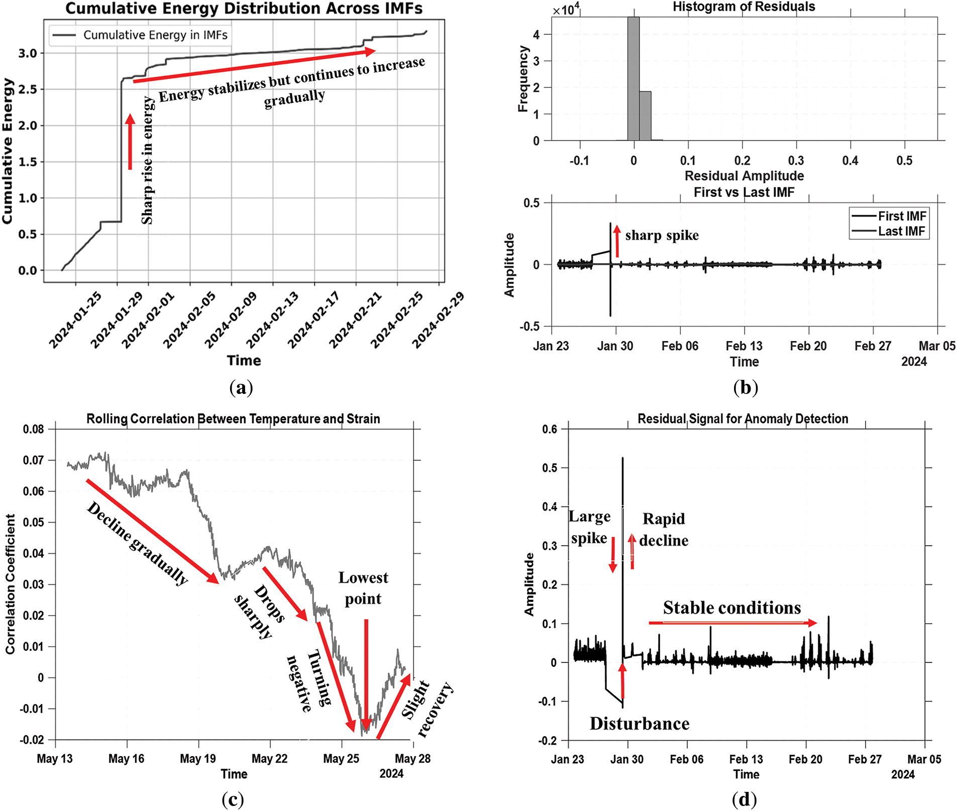
Figure 12: The SPWL sensor results over time. (a) Cumulative energy distribution across IMFs; (b) Histogram of residual amplitudes and the first and last IMFs; (c) Correlation coefficient between temperature and strain; (d) Residual signal from anomaly detection

In this figure, the gray curve depicts an upward trend in cumulative energy, with noticeable spikes followed by phases where the energy levels out or rises gradually. A marked increase in cumulative energy occurs around 28–29 January 2024, hinting at a significant event or shift in structural behavior, like a load impact or a sudden stress response. Following this sharp surge, the energy stabilizes but continues to rise slowly through early to mid-February. This suggests that there aren’t any major incidents during that time, just minor fluctuations or disturbances. The subsequent stabilization indicates that the structure likely returned to normal, as the external event seems to have passed, and the structure isn’t responding dynamically anymore. By the end of February, energy levels approach a plateau, signaling that the system is reaching a nearly steady state. Overall, tracking cumulative energy across IMFs can be useful for pinpointing times of structural weakness or deterioration. Sudden increases might imply ongoing damage or fatigue, while stabilization suggests normal operation. Keeping an eye on this energy distribution also helps engineers notice unusual responses and gives insights into the structure’s dynamic nature, which is critical for spotting anomalies, assessing damage, and ensuring safety in a structural health monitoring (SHM) system.

The upper graph in Fig. 12b presents a histogram of residual amplitudes, where most values cluster around zero. This indicates that the IMFs are successfully capturing the signal’s key features, with minimal unexplained variance. The X-axis shows the residual amplitude, while the Y-axis illustrates how frequently each amplitude occurs.

The histogram features a pronounced spike around the zero residual amplitude, suggesting most residuals are indeed very close to zero. It does appear slightly skewed to the right, with a small tail extending towards larger positive residuals (up to 0.5). This points to the fact that while most residuals hover near zero, a few instances exist where the model underestimates observed values (these are the positive residuals). The slight positive skew might indicate that in some cases, the structure shows larger responses than what the model predicts, which could signal potential issues or behaviors that the model doesn’t fully account for. This might warrant further investigation for any damage or unusual structural behavior. The histogram of residuals suggests that the predictive model is generally performing well, given that most residuals are near zero. However, that slight right skew could suggest some under-predictions that may require additional analysis.

The lower graph in Fig. 12b shows a comparison of the amplitudes for the first and last intrinsic mode functions (IMFs) over time. The X-axis represents time, while the Y-axis shows the amplitude of the IMFs.

The first IMF, highlighted in black, usually picks up the highest-frequency signals. In this case, there’s a noticeable spike around January 30, which likely indicates a significant high-frequency event—maybe due to some structural issue, damage, or added stress. After that spike, the first IMF levels off, with only minor shifts, suggesting that there are just small responses or some noise. On the other hand, the last IMF, shown in red, pretty much stays at zero for the entire monitoring period. This reflects a stable, low-frequency behavior of the structure, indicating that there weren’t any major low-frequency changes with the bridge throughout this time. The spike in the first IMF might hint at a structural problem that needs a closer look, while the steadiness of the last IMF suggests the bridge’s low-frequency behavior is steady. This analysis illustrates how IMFs can effectively capture both swift and gradual changes in the structural response, aiding in assessing the health of the structure over time.

Moving on to Fig. 12c, it illustrates the relationship between strain and temperature over time, with time spanning from May 13 to May 28, 2024, and the Y-axis showing correlation coefficient values.

The bright gray line in Fig. 12c tracks how the correlation coefficient shifts during this period. Starting around May 13, the coefficient is positive, sitting around 0.07, showing a fairly strong positive correlation at the outset. However, after May 14, there’s a gradual decline, which points to a weakening correlation. This downward trend persists until about May 19. Then, around May 22, the correlation coefficient drops more dramatically and turns negative by May 24. This shift from positive to negative implies a reversal or a big change in the relationship being analyzed. By May 25, the correlation hits its lowest around −0.02, indicating a slight negative correlation. There’s a minor bounce back after that, trending upward toward May 28, but it still remains below zero. This decline in correlation might suggest a change in the structural condition or a shift in how the two variables relate. The move from positive to negative correlation could signal the beginning of structural changes or damage, resulting in a different dynamic response. The lowest point, with a negative correlation, could indicate an unusual condition or a stress point in the structure, followed by some recovery observed later. The slight recovery towards the end of May could hint at stabilization, but it doesn’t fully return to earlier correlation levels. Keeping an eye on these correlation trends can help engineers spot early signs of structural issues and understand how the measured variables are interacting, which is crucial for maintaining structural safety and performance.

Fig. 12d illustrates how a residual signal’s amplitude changes over time, with time represented on the X-axis and amplitude on the Y-axis.

The black line in Fig. 12d shows the amplitude fluctuating throughout this period. Notably, around January 30, there’s a significant spike in amplitude, hitting nearly 0.6, which probably signals a major event like a sudden load, impact, or even structural damage. Following this spike, the amplitude drops quickly, creating a clear peak in the signal. This suggests there was some important disturbance during that time, possibly hinting at a sudden change in the monitored structure or system. The sharpness of this spike indicates it might have been a short yet powerful event. Afterward, the signal settles back to lower amplitude levels, indicating a return to normal conditions. However, the increasing fluctuations seen towards the end of February could mean ongoing shifts or instabilities that might need further inquiry to see if the structure is gradually degrading or showing new dynamic behavior. After the spike, the amplitude stabilizes at a much lower range, hovering close to zero with minor variations through early February. This phase of low amplitude likely implies a return to stable conditions following the disturbance.

Fig. 13a shows the cross-covariance between temperature and strain over a range of time lags from −2000 to 2000. The oscillating pattern in Fig. 13a, alternating between positive and negative values, suggests a periodic relationship between the two signals. The strong peaks around zero lag indicate a high correlation when the signals are aligned or have very little time difference, showing they’re closely linked in timing. The symmetry around zero lag reinforces this, illustrating that the correlation looks similar whether one signal leads or lags the other. As the lag increases, the amplitude of the cross-covariance gradually decreases, pointing to a weakening correlation over time. This analysis indicates that these signals, likely from different sensors, are closely related when events happen simultaneously, with a periodic nature that probably connects to cyclic structural responses. Understanding this timing relationship helps in evaluating structural dynamics and spotting potential abnormalities.

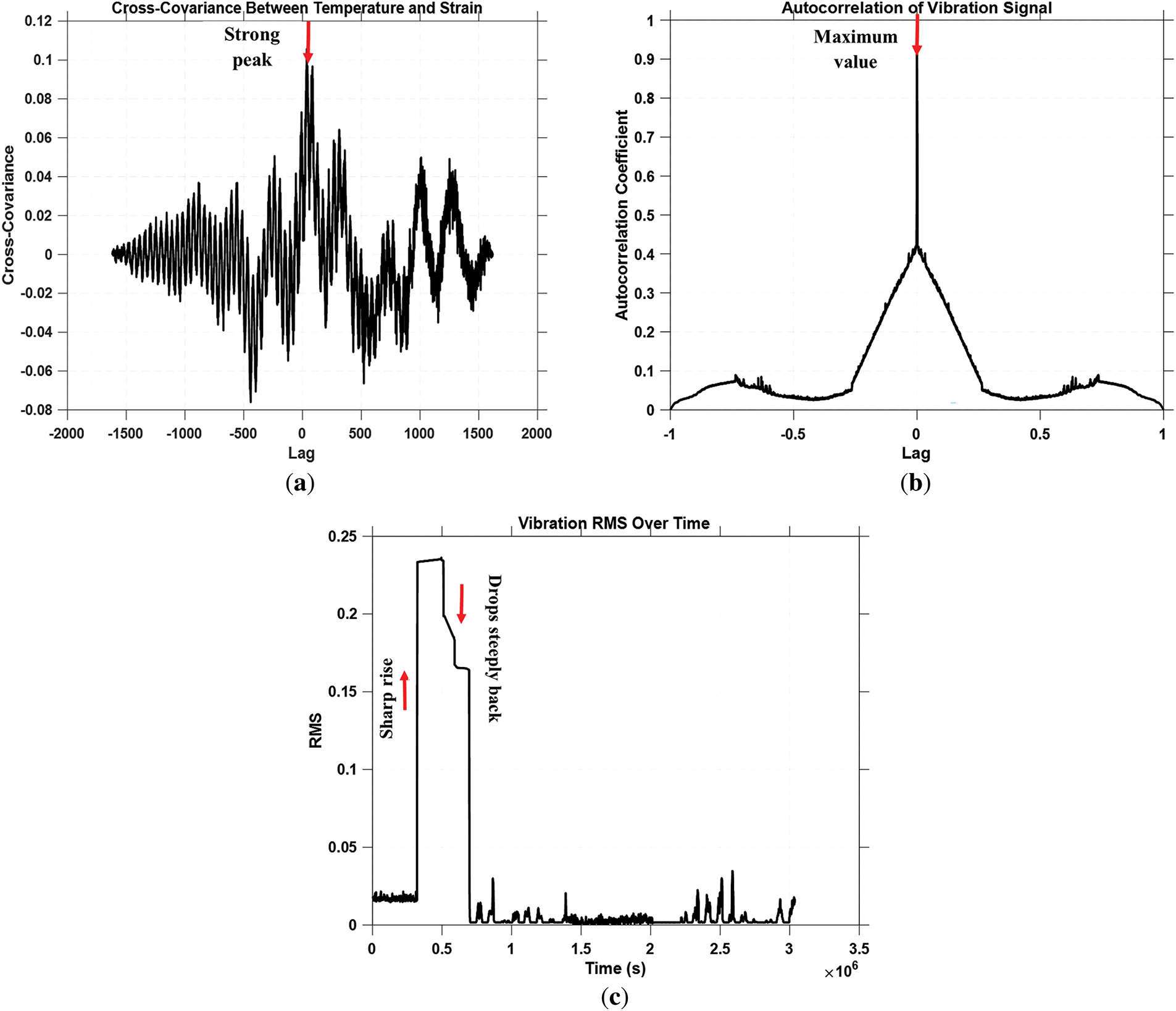
Figure 13: The SPWL sensor results over time. (a) Cross-covariance between temperature and strain; (b) autocorrelation of vibration signal; (c) root mean square (RMS) of a vibration signal

Fig. 13b illustrates the autocorrelation coefficient on the Y-axis as a function of lag on the X-axis, spanning from −1 to 1. At zero lag, the coefficient peaks at almost 1, showing a perfect correlation of the signal with itself. The plot in Fig. 13b is symmetric around the zero lag point, indicating that the signal behaves similarly for both positive and negative time shifts. As lag increases in either direction, the autocorrelation coefficient drops, meaning the correlation weakens as the time difference between the signal and its delayed version grows. Smaller peaks around ±0.5 lag suggest some degree of periodicity or repetitive behavior in the signal, hinting that it might oscillate at regular intervals. This could point to cyclical behavior in the monitored structure. A typical decline in autocorrelation with increasing lag indicates that earlier values gradually lose their influence over time. This analysis can highlight patterns like periodic structural responses or consistent cyclic loading. The sharp peak at zero lag reflects strong predictability and consistency in the signal, while smaller peaks at non-zero lags might suggest periodic influences that could help detect regular dynamic behavior or emerging structural issues.

Fig. 13c represents the Root Mean Square (RMS) value of a vibration signal over time, with the Y-axis showing the RMS amplitude and the X-axis representing time. In the initial part of the time window (0 to about 0.5 s), the RMS value spikes sharply to around 0.25. This suggests some significant disturbance occurred early in the signal, leading to a high level of energy or activity. Following that peak, the RMS amplitude rapidly falls back to near-zero, indicating that the disturbance calmed down quickly, and the signal returned to a low-energy state. The subsequent drop in RMS and the extended period of low values suggest that after the initial disturbance, the structure returned to a stable state with minimal activity. From 1 to 2.5 s, the RMS stays low, dotted with small spikes, indicating a stable period with little dynamic activity or fluctuations in the signal. Toward the end of the time window (around 2.5 to 3 s), there are minor but more frequent spikes in the RMS value, signaling renewed dynamic activity or slight disturbances in the bridge. Overall, keeping an eye on the RMS of signals is vital in Structural Health Monitoring (SHM), as it helps detect changes in the structure’s energy levels and identify potential disturbances or reactions over time.

5  Conclusions

This paper successfully achieved comprehensive perception and real-time monitoring of important infrastructure by developing SPWL sensors and building a bridge SHM system. The application of this technology not only improves the safety and efficiency of highway operations, but also brings revolutionary changes to the field of structural health monitoring. In the future, with the continuous development and improvement of data analysis technology, we will be able to more accurately assess the health of infrastructure and provide more solid technical support for the development of intelligent transportation and intelligent infrastructure.

6  Future Work

The analysis using IMF decomposition and RMS is informative. Nevertheless, a deeper explanation of how these results correlate with potential structural issues (e.g., fatigue, crack formation) would improve the technical insight. In future work, it is suggested to investigate the effect of the potential structural issues on the SPWL sensors’ measurements and structural identifications using artificial intelligence. A collection of Machine Learning Methods for classification and compared to their application will be used, these methods are Logistic Regression, K-Nearest Neighbors, Decision Tree, Support Vector Machine, Gaussian, and Stacking methods.

Acknowledgement: None.

Funding Statement: The author received no specific funding for this study.

Availability of Data and Materials: Not applicable.

Ethics Approval: Not applicable.

Conflicts of Interest: The author declares no conflicts of interest to report regarding the present study.

References

1. Kopiika N, Di Bari R, Argyroudis S, Ninic J, Mitoulis SA. Sustainability and resilience-driven prioritisation for restoring critical infrastructure after major disasters and conflict. Transp Res Part D Transp Environ. 2025;139(2):104592. doi:10.1016/j.trd.2025.104592. [Google Scholar] [CrossRef]

2. Forcellini D, Mitoulis SA. Effect of deterioration on critical infrastructure resilience—framework and application on bridges. Results Eng. 2025;25(1):103834. doi:10.1016/j.rineng.2024.103834. [Google Scholar] [CrossRef]

3. Padgett JE, Tapia C. Sustainability of natural hazard risk mitigation: life cycle analysis of environmental indicators for bridge infrastructure. J Infrastruct Syst. 2013;19(4):395–408. doi:10.1061/(asce)is.1943-555x.0000138. [Google Scholar] [CrossRef]

4. Zhang C, Xu Y, Silik A, Li H, Noori M, Altabey WA. Analysis of instantaneous frequency for structure condition tracking using time-frequency representation: comparative study. In: Proceedings of the 22nd International Scientific Conference, Engineering for Rural Development; 2023 May 24–26; Jelgava, Latvia. doi:10.22616/ERDev.2023.22.TF212. [Google Scholar] [CrossRef]

5. Guo D, Hong W, Altabey WA. Pavement pothole monitoring via computer vision technology. In: Proceedings of the 2023 IEEE International Smart Cities Conference (ISC2 2023); 2023 Sep 24–27; Bucharest, Romania. doi:10.1109/ISC257844.2023.10293626. [Google Scholar] [CrossRef]

6. Guo D, Hong W, Altabey WA. Intelligence approach for structural monitoring via UAV-artificial intelligence-based. In: Proceedings of the 2023 IEEE International Smart Cities Conference (ISC2 2023); 2023 Sep 24–27; Bucharest, Romania. doi:10.1109/ISC257844.2023.10293349. [Google Scholar] [CrossRef]

7. Fujino Y. Vibration, control and monitoring of long-span bridges—recent research, developments and practice in Japan. J Constr Steel Res. 2002;58(1):71–97. doi:10.1016/S0143-974X(01)00049-9. [Google Scholar] [CrossRef]

8. Xie Y, Zhang S, Meng X, Nguyen DT, Ye G, Li H. An innovative sensor integrated with GNSS and accelerometer for bridge health monitoring. Remote Sens. 2024;16(4):607. doi:10.3390/rs16040607. [Google Scholar] [CrossRef]

9. Wang Y, Wang J. Research on socket communication system based on ZigBee wireless sensor network. In: Proceedings of the 7th International Conference on Computer Engineering and Networks (CENet2017); 2017 Jul 22–23; Shanghai, China. doi:10.22323/1.299.0024. [Google Scholar] [CrossRef]

10. Lin L, Li X, Gu W. PM2.5 monitoring system based on ZigBee wireless sensor network. IOP Conf Ser Earth Environ Sci. 2017;69(1):012094. doi:10.1088/1755-1315/69/1/012094. [Google Scholar] [CrossRef]

11. Phan LA, Kim T, Kim T, Lee J, Ham JH. Performance analysis of time synchronization protocols in wireless sensor networks. Sensors. 2019;19(13):3020. doi:10.3390/s19133020. [Google Scholar] [PubMed] [CrossRef]

12. Wu J, Zhang L, Bai Y, Sun Y. Cluster-based consensus time synchronization for wireless sensor networks. IEEE Sens J. 2015;15(3):1404–13. doi:10.1109/JSEN.2014.2363471. [Google Scholar] [CrossRef]

13. Yildirim KS, Kantarci A. Time synchronization based on slow-flooding in wireless sensor networks. IEEE Trans Parallel Distrib Syst. 2014;25(1):244–53. doi:10.1109/TPDS.2013.40. [Google Scholar] [CrossRef]

14. Song C, Xia K, Xu Z. A self-supported structure hybrid triboelectric/piezoelectric nanogenerator for bio-mechanical energy harvesting and pressure sensing. Microelectron Eng. 2022;256(11):111723. doi:10.1016/j.mee.2022.111723. [Google Scholar] [CrossRef]

15. Xia K, Xu Z, Zhu Z, Zhang H, Nie Y. Cost-effective Copper–Nickel-based triboelectric nanogenerator for corrosion-resistant and high-output self-powered wearable electronic systems. Nanomater. 2019;9(5):700. doi:10.3390/nano9050700. [Google Scholar] [PubMed] [CrossRef]

16. Xia K, Zhu Z, Zhang H, Du C, Wang R, Xu Z. High output compound triboelectric nanogenerator based on paper for self-powered height sensing system. IEEE Trans Nanotechnol. 2018;17(6):1217–23. doi:10.1109/TNANO.2018.2869934. [Google Scholar] [CrossRef]

17. Xia K, Wu D, Fu J, Hoque NA, Ye Y, Xu Z. Tunable output performance of triboelectric nanogenerator based on alginate metal complex for sustainable operation of intelligent keyboard sensing system. Nano Energy. 2020;78:105263. doi:10.1016/j.nanoen.2020.105263. [Google Scholar] [CrossRef]

18. Fu J, Xia K, Xu Z. Double helix triboelectric nanogenerator for self-powered weight sensors. Sens Actuat A Phys. 2021;323:112650. doi:10.1016/j.sna.2021.112650. [Google Scholar] [CrossRef]

19. Xia K, Zhu Z, Zhang H, Du C, Wang R, Xu Z. Cost-effective triboelectric nanogenerator based on teflon tape and conductive copper foil tape. Microelectron Eng. 2018;199(4):114–7. doi:10.1016/j.mee.2018.08.002. [Google Scholar] [CrossRef]

20. Xia K, Yu M. Highly robust and efficient metal-free water cup solid–liquid triboelectric nanogenerator for water wave energy harvesting and ethanol detection. Chem Eng J. 2025;503(3):157938. doi:10.1016/j.cej.2024.157938. [Google Scholar] [CrossRef]