Defect Detection of Wind Turbine Blades Using Multiscale Feature Extraction and Attention Mechanism

1  Introduction

Wind power generation, as a clean, renewable energy source, is increasingly widely used in the current global energy transition [1]. In wind power generation systems, the blades of wind turbines are crucial components that efficiently convert wind energy into mechanical energy, which is then converted into electrical energy. Once a safety problem occurs in a wind turbine blade, such as a fracture owing to reduced structural strength, the consequences will be unimaginable. On land, the broken blade may fall and smash into surrounding facilities and farmland, endangering nearby personnel and posing a significant threat to property. In the sea, the falling blade will damage the marine ecosystem and may even affect the navigation of other ships. At the same time, the failure of the blades will cause the entire wind turbine to stop functioning, affecting power generation efficiency and leading to instability in the power supply, with a profound negative impact on the production and daily life of areas reliant on wind power. Therefore, to ensure that wind power projects operate safely, reliably, and efficiently, it is essential to conduct comprehensive, detailed, and scientific safety inspections of wind turbine blades, promptly identify potential safety hazards, and implement appropriate repair measures. Additionally, the accuracy of wind turbine blade defect detection is critical. Low detection accuracy leads to numerous false negatives, where blades with actual defects—such as oil leakage, lightning strike, erosion, or tape breakage—are incorrectly classified as defect-free during inspection. Such misjudgments accelerate deterioration under repeated alternating loads and persistent erosion from extreme weather. Simple defects gradually evolve into deep cracks, core delamination, and other severe issues. Ultimately, this not only heightens the risk of structural failures, such as blade fractures and leading-edge delamination, which lead to abnormal shutdowns and prolonged maintenance interruptions, but may also escalate into catastrophic accidents, including high-altitude blade breakage or turbine overturns. It not only incurs substantial economic losses from equipment repairs and replacements, as well as power generation losses, but also risks casualties among on-site maintenance personnel. The safety costs and economic impacts are incalculable.

Wind turbine blade inspection is primarily divided into noninvasive testing [2,3] and visual inspection methods [4]. Non-destructive testing methods include ultrasonic testing [5], X-ray testing [6], acoustic emission testing [7], and infrared thermography testing [8,9]. Ultrasonic and X-ray testing typically require expensive X-ray or ultrasonic emission equipment. The equipment’s procurement cost is high, and for some smaller wind power enterprises or testing organizations, purchasing it is a considerable economic burden. The acoustic emission detection process is complex and requires professional labor with rigorous training to operate accurately. Once the operator error occurs, there may be a misjudgment. Infrared thermal imaging detection technology is more demanding in terms of environmental requirements. In the external environment, if the temperature change is not significant, light interference is substantial, or the wind blade surface temperature difference is slight, it becomes difficult to accurately detect defects. Appearance inspection methods are mainly divided into manual visual inspection and drone inspection. Artificial visual inspection is generally performed in the wind turbine shutdown state by an inspector using binoculars to observe the wind turbine blade condition and record any cracks, scratches, breakage, and other markings. Manual visual inspection is both simple and easy to execute [10], but it relies heavily on the experience and technical level of the inspectors, and the inspection efficiency is low, making it unsuitable for inspecting large-area wind power plants. Drone inspection [11–13] utilizes drones equipped with high-resolution imaging systems or other sensing technologies to capture detailed surface images of wind turbine blades. It then detects surface imperfections on the blades by analyzing and processing the collected images. Drone inspection is highly efficient, and advances in computer vision technology have gradually improved detection accuracy.

In the uncrewed aerial vehicle (UAV) inspection method, a deep learning-based target detection algorithm is employed to detect defects on wind turbine blades. In recent years, researchers have studied defect-detection algorithms for wind turbine blades. Deng et al. [14] used a support vector machine (SVM) classification approach to detect and categorize defects in wind turbine blades, optimizing the training process through a particle swarm optimization algorithm combined with flight strategies. The recognition rate can reach 92%; however, the detection time is lengthy, making it challenging to meet real-time detection requirements. Gao et al. [15] applied an algorithm for target detection based on deep learning to locate defects in wind-turbine blades. The self-DIstillation with NO labels (DINO) model was enhanced by replacing the backbone with Residual Neural Network (ResNet) 18, introducing an efficient channel attention (ECA) module as an attention mechanism, and adding an encoder layer with multi-head attention to the encoder’s last layer. The final model achieved a detection accuracy of 93.2% and a recall performance of 93.6% for identifying wind turbine blade damage, while maintaining a processing speed of up to 27 frames per second. However, no model-complexity parameter is provided in this paper to determine whether it can be deployed on edge devices for real-time detection. The detection speed is low, making its application for real-time surveillance of uncrewed aerial vehicles difficult. Masita et al. [16] employed three convolutional neural networks with residual modules, namely Residual Convolutional Neural Network with three Residual Blocks (Res-CNN3), to detect defects in wind turbine blades. The defect identification model, Res-CNN3, designed for wind turbine blades, achieved a mean average precision (mAP) of 80.6%, with 51.7 M parameters and an average test time of 0.036 s. The model has too many parameters, requires substantial computational resources, and exhibits slower recognition speed. Ran et al. [17] enhanced the YOLOv5s algorithm by incorporating weighted feature fusion and cross-scale connectivity, thereby improving the feature pyramid network through a coordinate-based attention strategy. This increased the model’s defect-detection accuracy for wind turbine blades by 4%. However, with a model size of 11.6 M, the model consumes substantial storage space, and deployment costs increase accordingly. Gohar et al. [18] used a slice-assisted inference model to detect defects in wind-turbine blades. By comparing the detection in different scenarios, they concluded that the model has a significant advantage for ultra-high-definition image datasets and small-target detection. Still, the paper did not provide the parameters related to the model’s complexity, and there is no way to know whether it can be deployed in edge or embedded devices with limited computational resources. Lv et al. [19] enhanced the ResNet backbone architecture using the single-shot multiBox detector (SSD) framework. The improved backbone network employs a connectivity network comprising a factorization depth-separable bottleneck and a feature aggregation module. It proposed a bidirectional feature pyramid network (BiFPN), a bi-directional cross-scale feature pyramid that balances accuracy and computation time. However, the dataset contains only three defect types—gel coat peeling, surface cracking, and surface corrosion—relatively few compared to the actual wind turbine blade defects that need to be detected.

As mentioned above, advancements in deep learning techniques for identifying wind turbine blade defects have been achieved; however, certain limitations remain. For example, the effective extraction of feature parameters in complex images for more accurate defect detection in wind turbine blades, achieving an effective balance between detection accuracy and model complexity to meet the deployment of embedded devices or edge devices, and maintaining a high detection rate to fulfill the requirement for real-time defect analysis in wind turbine blades on UAVs, is critical for practical applications. To address the aforementioned challenges, this study introduces a wind turbine blade defect detection model, WtCS-YOLO11, incorporating multiscale feature extraction and an attention mechanism. The primary innovations of this study are summarized as follows:

(1)   When wavelet convolution was introduced into the C3k2 module of the YOLO11 model, the module was restructured as C3k2_WTConv. Notably, wavelet convolution decomposes features across multiple scales, enabling the effective capture of global contextual information in wind turbine blade images. This capability facilitates the extraction of multiscale features, ultimately enhancing detection accuracy.

(2)   Improving the YOLO11 model by incorporating the CBAM attention mechanism. The CBAM module combines channel and spatial attention. It emphasizes key features, suppresses irrelevant ones, enhances the model’s decision-making ability, facilitates the identification of significant defects in wind turbine blades, and improves the detection accuracy of wind turbine blade defects. There has been no surge in model complexity and size.

(3)   The normalized Wasserstein distance and shape-aware intersection over union (NWD-Shape-IoU) module was constructed by combining the NWD distance and Shape-IoU, and applied to the YOLOv11 model. Shape-IoU accounts for both the scale and shape of the bounding box, while the NWD distance provides a more precise measure of bounding box similarity.

(4)   The C3k2_WTConv module, CBAM attention mechanism, and NWD-Shape-IoU module were simultaneously integrated into the YOLO11 model to enhance it. In wind turbine blade defect detection, mAP50 was improved by 2.4%. Detection accuracy was significantly improved with no increase in model complexity or size.

2  Methods

2.1 YOLO11 Model

YOLO11 is a newer version of the YOLO series, released on 30 September 2024. YOLO11 introduces innovations based on the previous YOLO series, achieving further improvements in detection accuracy while reducing the network’s parameter count [20]. Due to the streamlined model structure, YOLO11’s inference speed is also enhanced, resulting in higher real-time performance. YOLO11 is sufficiently robust to be applied to a range of tasks, including target recognition, image classification, image segmentation, and pose estimation. This provides a powerful and practical solution for real-world applications [21].

The structure of the YOLO11 model is depicted in Fig. 1 and features three main improvements [22] over the previous YOLO generation, namely YOLOv8. First, YOLO11 uses a C3k2 module instead of a cross-stage partial with two convolutions (C2f) module. The C3k2 module uses a customized C3k block (with two convolutions) instead of the standard bottleneck block used in the C2f module.

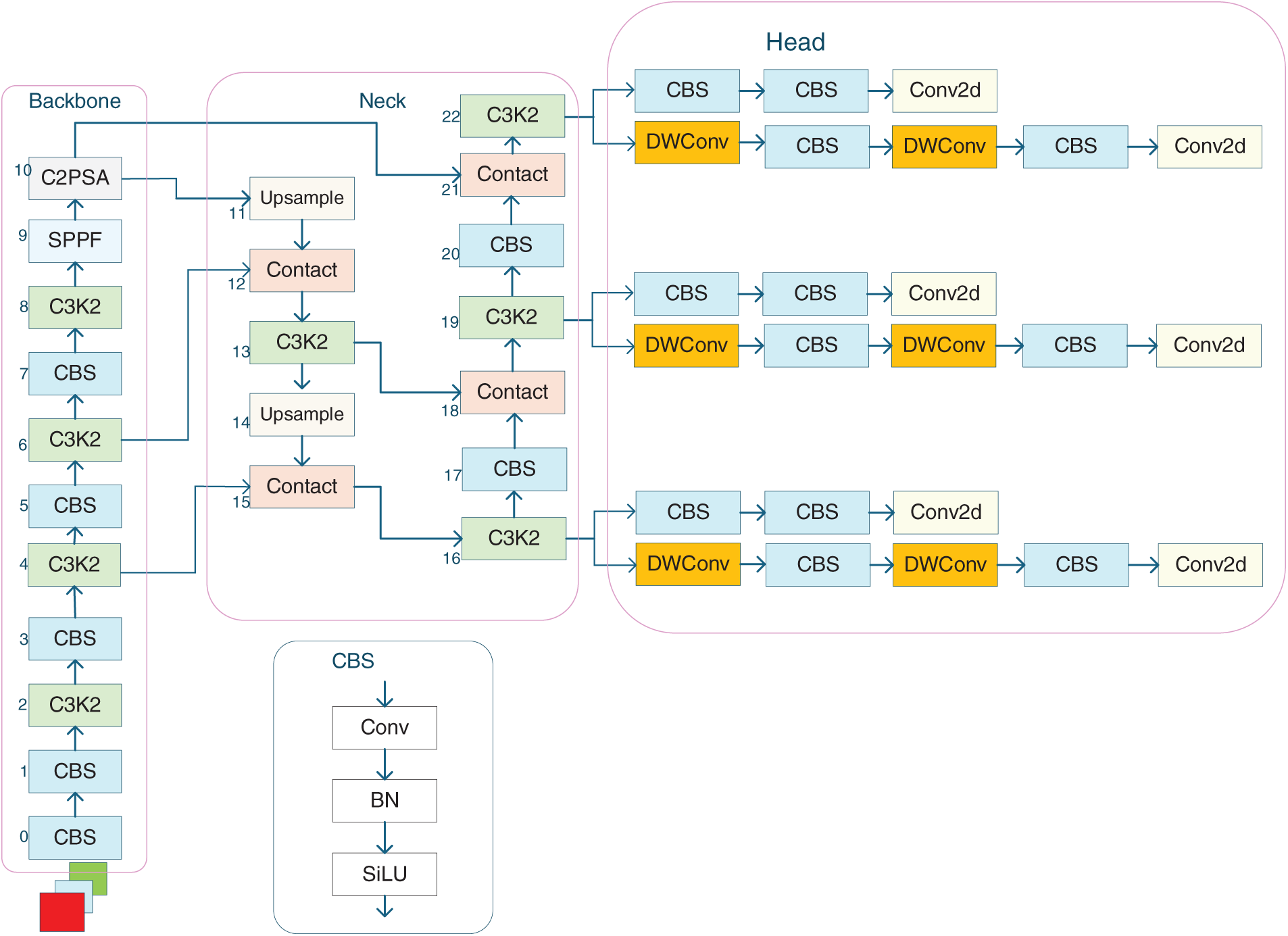
Figure 1: YOLO11 model architecture diagram

This enhances feature learning and reduces computation by learning across phases. The C3k2 module implements a cascade connection of two cross-stage partials with 3 × 3 kernels (C3k) modules, effectively increasing the receptive field. The C3k2 module adopts a parallel configuration of two C3k modules. The input feature map is fed into both independent C3k modules simultaneously for processing. Each C3k module maintains the same number of output channels as its input. Subsequently, the feature maps from these two modules are concatenated along the channel dimension, ultimately forming an output feature map with two channels. This effectively doubles the network width and enhances its capacity. This architecture further improves the module’s feature extraction capabilities and efficiency. This structure further enhances the module’s ability and efficiency in extracting features. Second, the cross-stage partial with pyramid spatial attention (C2PSA) module was added to YOLO11. It embeds a multi-head attention mechanism within the cross-stage partial with two convolutions (C2) mechanism, thereby enhancing the module’s ability to extract key features. Finally, the detection head of YOLO11 follows the decoupled detection head of YOLOv8. A depthwise convolution (DWConv) is added to the classification-detection head to reduce computation [23]. The innovations and improvements in YOLO11 effectively improve detection efficiency and accuracy.

2.2 Proposed Methodology

Although the YOLO11 model is well applied, the target defect size varies significantly in the field of wind turbine blade defect detection. The target categories included both large and small targets; therefore, YOLO11’s detection performance is limited. Further optimization and enhancement of the model are required to achieve higher detection accuracy. In this thesis, three main improvements were made to the YOLO11 model. First, the C3k2_WTConv module is introduced as a substitute for the C3k2 module in the neck network, increasing the convolutional module’s receptive field and effectively capturing both global and local features, making it effective for recognizing multiscale and small targets in wind turbine blade images. Second, the CBAM attention module is introduced at the end of the neck network. The CBAM module comprises channel and spatial attention, which enhance the feature map’s processing capacity, allowing the network to focus more effectively on key feature representations and facilitating the detection of large targets. Third, the bounding box regression loss adopts Shape-IoU combined with NWD distance, which considers not only the positional relationship between the predicted box and the ground truth box, but also incorporates the shape and scale of the bounding box into the loss function, while measuring their similarity using the NWD distance, which makes the bounding box regression more accurate. The structure of the improved algorithm is illustrated in Fig. 2.

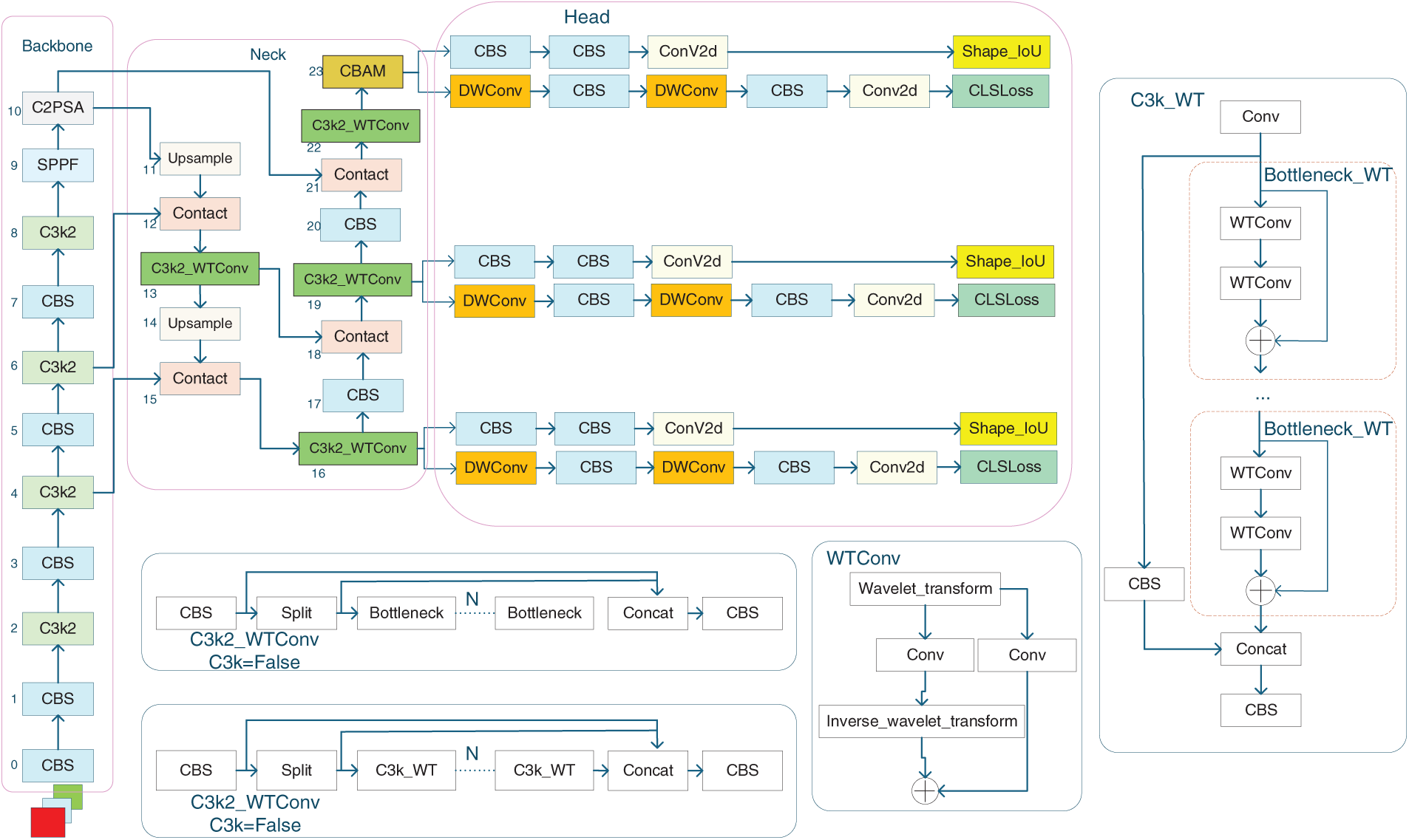
Figure 2: Architecture of the WtCS-YOLO11 model

2.2.1 C3k2_WTConv

The C3k2_WTConv module replaces the convolutional layer in the C3k2 module with a wavelet convolutional layer (WTConv). The traditional convolutional module in the C3k2 module is limited by the convolutional kernel size, making it difficult to efficiently capture global context from features, thereby affecting target recognition. Although this problem can be mitigated to some extent by increasing the convolutional kernel size in recent years, larger kernel sizes lead to a surge in the number of parameters. This can simultaneously increase the number of parameters, which makes the model less suitable for deployment on edge devices. By integrating the wavelet transform module WTConv into the convolutional network, it can achieve a large receptive field without overparameterization, extract multiscale features across different frequency bands, and effectively improve model performance without increasing model complexity.

When selecting wavelet basis functions, it is crucial to accurately extract high-frequency edge features, such as tape damage and lightning strike, for wind turbine blade defect detection while meeting the real-time and lightweight requirements of edge devices on drones. To validate the appropriateness of choosing the Haar wavelet, we compare it with commonly used domain-specific basis functions—Daubechies 4 (db4), Symlets 4 (sym4), and Coiflets 2 (coif2)—based on core characteristics and deployment advantages. The results are presented in Table 1.

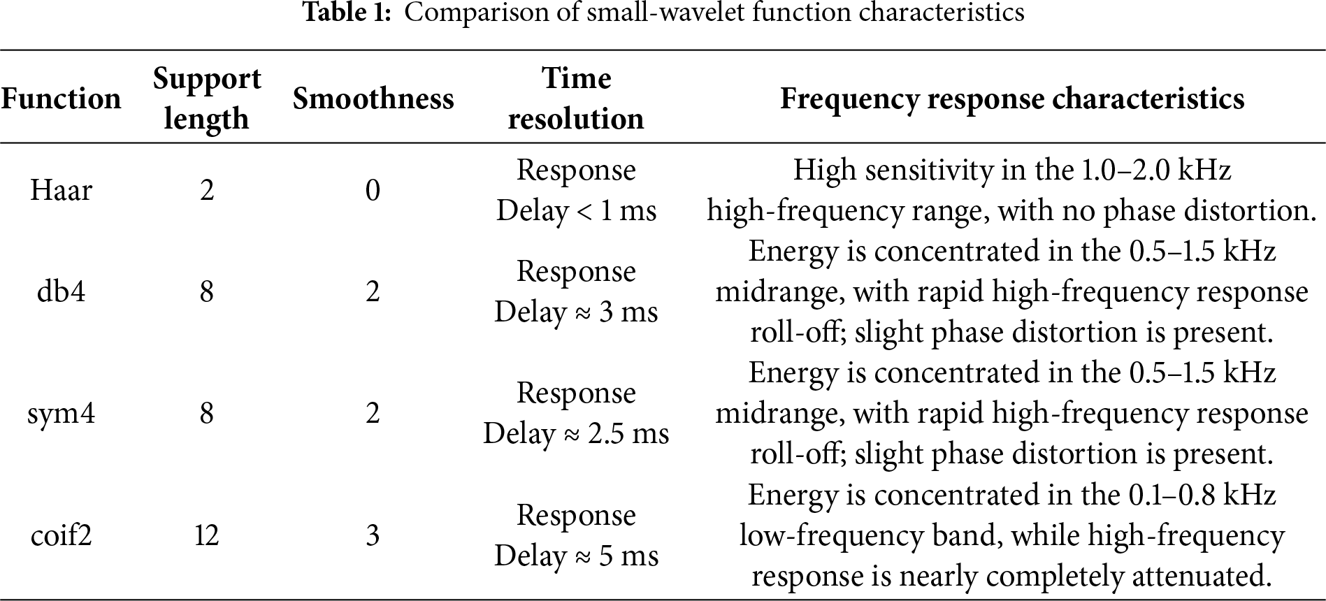
The edges of tape breakage defects exhibit distinct characteristics, with frequency domain energy concentrated in the high-frequency band of 1.0–1.8 kHz. This requires basis functions with high temporal resolution to pinpoint edge locations precisely. Lightning strike typically manifests as small-scale, high-contrast details, with frequency domain dispersion spanning 1.2–2.0 kHz. This requires the use of basis functions to maintain high response sensitivity at high frequencies. Soiling defects exhibit localized high-frequency textures, necessitating base functions that avoid excessive smoothing to preserve texture characteristics. Oil leakage and erosion exhibit mid-to-low-frequency features, although these defects account for only about 30% of actual inspections and can be supplemented and optimized through feature-fusion mechanisms. Paint loss is characterized by low-frequency, blurred defects.

In terms of scene adaptability, the high-frequency response of Haar wavelets closely matches the frequency-domain features of tape damage, lightning strikes, and contamination. Its shortest support length delivers the highest temporal resolution, enabling the capture of defect edges without lag during high-speed drone imaging. The square-wave morphology naturally aligns with steep defect edges, allowing the precise extraction of high-frequency features without complex computations. Simple averaging and interpolation logic not only drastically reduces model parameters and computational complexity but also ensures real-time responsiveness on edge devices. In contrast, other wavelet basis functions exhibit significant limitations in specific scenarios. While db4 and sym4 show slight advantages in low- to mid-frequency defect extraction, their high-frequency response attenuation increases core defect miss rates, thereby directly compromising real-time performance. Coif2, though suitable for paint-loss defects, completely loses its high-frequency defect-extraction capability, and its massive computational demands render edge deployment impractical. Furthermore, the symmetry of Haar wavelets prevents phase shifts during feature extraction, ensuring precise localization of defects. In contrast, the non-perfect symmetry of db4 and sym4 often leads to positional prediction errors for oblique defects, such as lightning strike, thereby increasing the risk of false positives.

The WTConv module leverages these advantages by applying the two-dimensional Haar wavelet transform to the convolution layer. It first performs a multi-level decomposition of the input image using four Haar wavelet filters, dividing it into four frequency bands [24]. This process can be described as follows:

[XLL,XLH,XHL,XHH]=WT(X)=Conv([fLL,fLH,fHL,fHH],X)(1)

here, XLL denotes a low-frequency component sub-band, XLH denotes a horizontal high-frequency component sub-band, XHL denotes a vertical high-frequency component sub-band, XHH denotes a diagonal high-frequency component sub-band, fLL denotes a low-frequency filter, fLH denotes a horizontal high-frequency filter, fHL denotes a vertical high-frequency filter, and fHH denotes a diagonal high-frequency filter.

The low-frequency subband captures low-frequency information in images, specifically areas with gradual pixel changes, such as the overall shape of wind turbine blades. It primarily focuses on image contours and boundaries, concentrating on large-scale features. The horizontal high-frequency subband mainly captures areas with significant horizontal pixel variations, such as the edge information of horizontally distributed defects on wind turbine blades. The vertical high-frequency subband primarily captures regions with significant vertical pixel variations, such as the edges of vertically oriented damage. The diagonal high-frequency subband mainly captures regions with pronounced diagonal pixel variations, such as textures or damage distributed diagonally across wind turbine blades [25]. These three high-frequency subbands are used to extract local image details, focusing on small-scale features.

WTConv then uses the inverse wavelet transform to construct the output after performing small-kernel deep convolution on the different frequency subband feature maps. Here, the convolution operation is performed not on the original image but on each of the four frequency bands using a small, deep convolution kernel. This wavelet-domain convolution method provides a larger receptive field, as shown in Fig. 3, which illustrates how WTConv handles low-frequency bands. A 3 × 3 convolution is performed on the low-frequency bands of the wavelet domain. The number of parameters of the secondary wavelet domain XLL(2) was nine, which corresponds to a 12 × 12 low-frequency receptive field in the response input X. The above frequency separation mechanism processes features across different frequency bands. The mid-to-low-frequency components, with their sensitivity to slowly varying information, contribute significantly to large-scale or overall shape defects, such as spots, while preserving contour information. High-frequency components focus on extracting small-scale details and local textures within the image. They are sensitive to minute, linear, or localized textural defects such as cracks, scratches, and pitting, effectively highlighting edges and minute features. Through the synergistic interaction of mid-to-low-frequency and high-frequency components, both global large-scale features and local small-scale features in wind turbine blade images are efficiently extracted, enabling feature extraction across different scales. As the wavelet transform reduces the spatial resolution of each sub-band, a small convolution kernel can cover a larger region of the original image, effectively enlarging the receptive field and enhancing target detection accuracy. Additionally, a small convolution kernel decreases the computational load of the parameters.

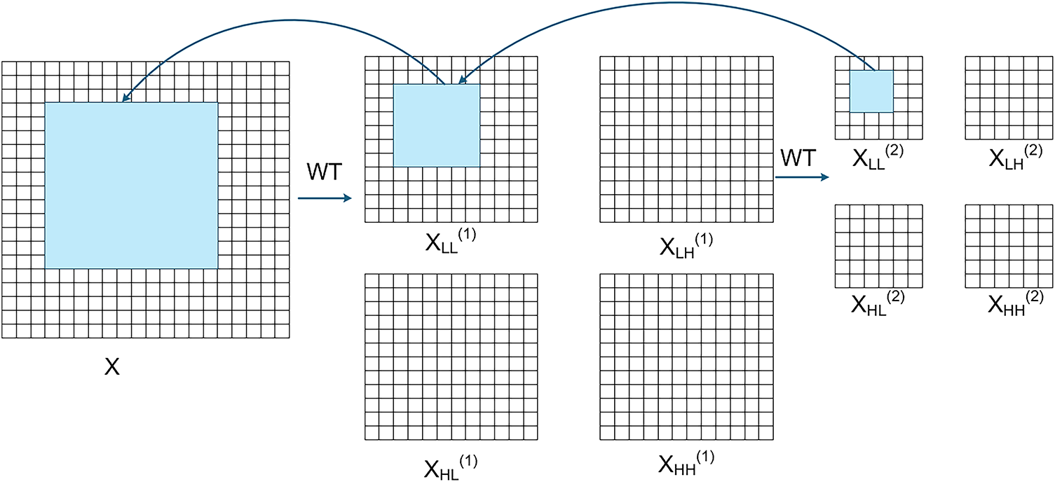
Figure 3: Diagram of the process of applying wavelet convolution to the low-frequency fractional quantum band

Floating-point operations (FLOPs) are defined as the total number of floating-point operations, encompassing both floating-point multiplication and floating-point addition. The FLOPs in the WTConv module are primarily composed of the combined FLOPs from three stages: two-dimensional Haar wavelet decomposition, subband deep convolution, and inverse Haar wavelet transform. The input feature map for the C3k2_WTConv module is denoted as F∈RH×W×C, where H represents the height of the feature map, W denotes its width, and C indicates the number of feature map channels. After two-dimensional Haar wavelet decomposition, four subbands of size RH2×W2×C2 are generated. The number of output channels M matches the number of input subband channels C.

During the two-dimensional Haar wavelet decomposition process, the row decomposition requires traversing H rows of the feature map, each row having a length of W. The computational effort for a single row is 2W, resulting in a total row decomposition FLOPs of 2HW. The column decomposition requires traversing the W columns of the feature map after row decomposition, each column having a height of H. The computational effort for a single column is 2H, resulting in a total column decomposition FLOPs of 2HW. The FLOPs for a single-channel 2D wavelet decomposition are 4HW. For a C channel feature map, the total FLOPs for 2D Haar wavelet decomposition are:

FLOPsWT=C×4HW=4CHW(2)

Deep convolution is performed on individual subbands after wavelet decomposition using a k×k small kernel, where k is typically set to 3. The computational logic for a single output pixel is as follows: First, element-wise multiplication between the convolution kernel and the input pixel is achieved through k2 floating-point multiplications. Then, the sum of the multiplication results is computed via k2−1 floating-point additions. Therefore, the total computational cost per output pixel is 2k2−1.

Depthwise convolution employs zero-padding to preserve feature map dimensions before and after the operation, with the output channel count M matching the input channel count C. Therefore, the total FLOPs formula for subband depthwise convolution is:

FLOPsDWConv=C×(2k2−1)×HW(3)

The inverse wavelet transform is the inverse operation of wavelet decomposition, reconstructing the original-sized feature map from four subbands. Its computational logic is entirely symmetric for wavelet decomposition, so the FLOPs of the inverse wavelet transform are equal to those of wavelet decomposition. The formula is:

FLOPsIWT=FLOPsWT=4CHW(4)

The FLOPs in the WTConv module are primarily composed of the combined FLOPs from three stages: two-dimensional Haar wavelet decomposition, subband deep convolution, and inverse Haar wavelet transform. Therefore, the FLOPs for the C3k2_WTConv module are:

FLOPsC3k2_WTConv=FLOPsWT+FLOPsDWConv+FLOPSIWT=(2k2+7)CHW(5)

The C3k2 module employs traditional convolutions, with FLOPs as follows:

FLOPsC3k2=2C2k2HW(6)

The typical number of channels C in the C3k2 module is 64, with k set to 3 and both H and W at 640. Substituting these values into Eqs. (5) and (6), the FLOPs for the C3k2 module are approximately 30.27 giga floating point operations (GFLOPs), while those for the C3k2_WTConv module are approximately 0.66 GFLOPs. It can be seen that the FLOPs of the C3k2_WTConv module have been significantly reduced, achieving lightweight processing while expanding the receptive field.

2.2.2 CBAM

To enhance the network’s ability to prioritize critical features and boost detection accuracy, this study introduces a CBAM attention mechanism that addresses the model’s constraints in handling information of varying scales and shapes. The CBAM module consists of a channel attention module and a spatial attention module, which enhance the model’s ability to perceive and emphasize crucial features by integrating channel and spatial attention mechanisms. Fig. 4 illustrates the flow chart of feature processing by the CBAM module. The CBAM module generates channel and spatial attention modules to process features. After processing, the newly generated feature map emphasizes the key features and suppresses irrelevant ones. The CBAM attention module dynamically recalibrates the importance of features across channels and spatial positions within the input feature map, focusing on the essential features such that the model automatically allocates attention to different regions, highlights the features of large targets, improves the model’s characterization ability and decision-making accuracy, and facilitates the detection of large targets.

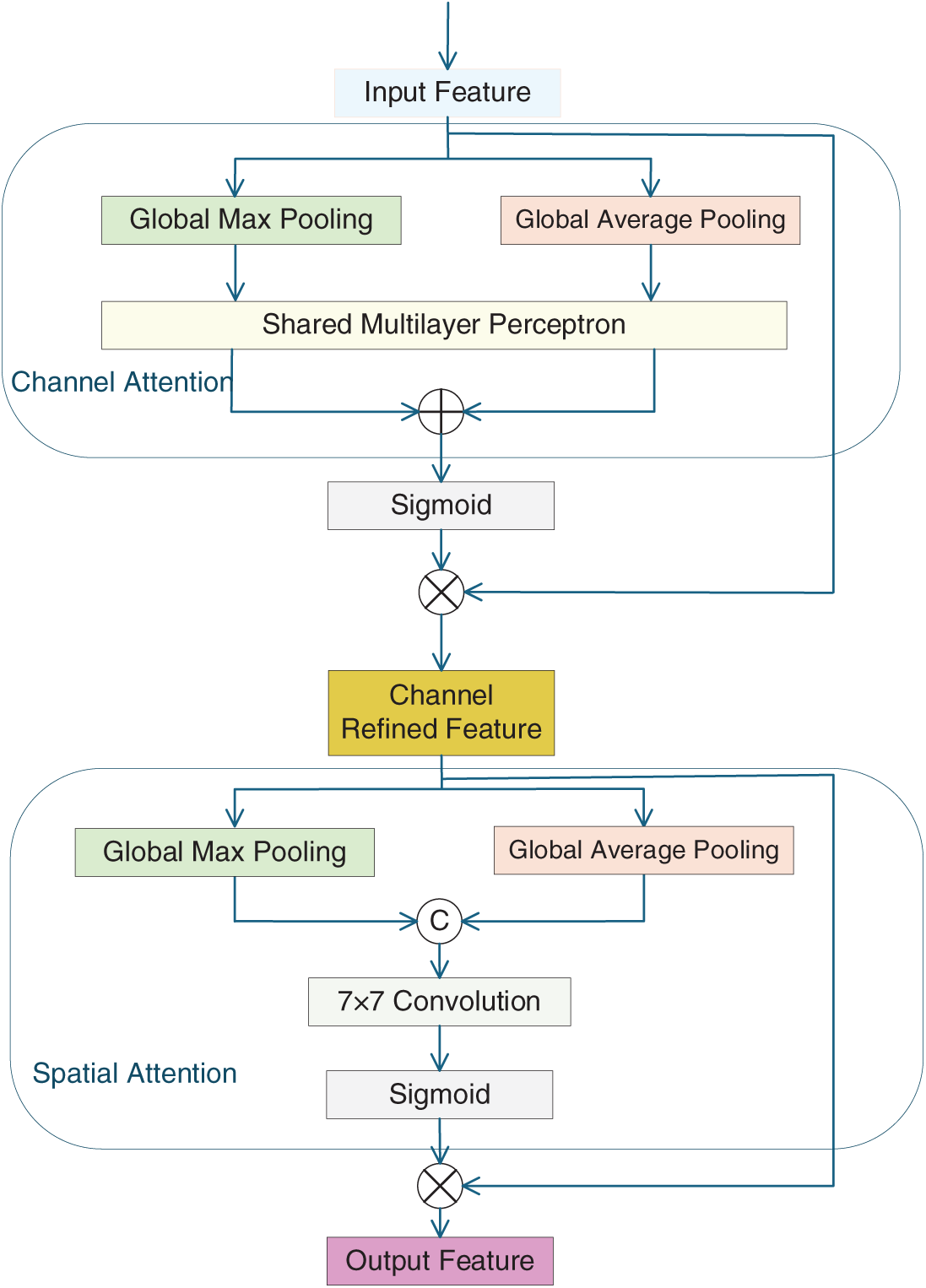
Figure 4: Flowchart of feature processing by the CBAM module

The detailed procedure is illustrated in Fig. 5, where the channel attention module initially applies global average pooling and max pooling to the feature map in the channel dimension [26,27], and then models the pooled vectors with the fully connected layer and the activation layer, and generates the attention weight vector for each channel, which enables the model to pay attention to the feature information of the essential channels and enhances the network’s ability to perceive different channels. The computational procedure is shown in Eq. (7).

Mc(F)=σ(MLP(AvgPool(F))+MLP(MaxPool(F)))=σ(W1(W0(Favgc))+W1(W0(Fmaxc)))(7)

where F∈RC×H×W is the input feature map, σ is the sigmoid function, and the Multilayer Perceptron (MLP) weights are W0 and W1, W0∈RC/r×C and W1∈RC×C/r.

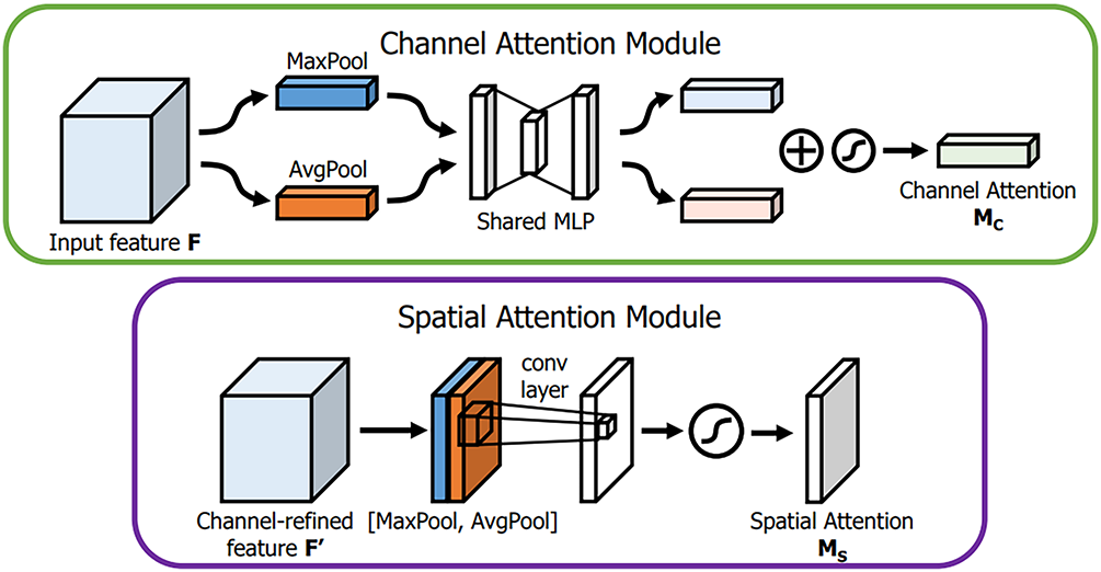
Figure 5: Schematic of each attention submodule

The spatial attention module first compresses the information on the channel dimension to the spatial dimension; the specific process is that the feature map is average pooled and maximally pooled along the channel axis to get two feature maps with spatial information, and then these two feature maps are spliced together to generate a new feature description, which is finally input into a convolutional layer to carry out feature fusion and extraction, and to generate a weight for spatial attention [28]. This process learns local feature patterns in space and mines the spatial relationships between different locations. The computation of the spatial attention module is described by Eq. (8).

Ms(F)=σ(f7×7([AvgPool(F′);MaxPool(F′)]))=σ(f7×7([F′savg;Fmax′s]))(8)

where σ is the sigmoid function and f7×7 denotes a 7 × 7 convolution kernel size.

2.2.3 NWD-Shape-IoU

Bounding box regression is a critical component of target detection, and the current bounding box regression in the YOLO11 model focuses solely on the spatial alignment between the ground truth and predicted boxes [29]. However, it does not account for the bounding box’s shape and scale. This approach may be practical in simple scenarios, but it is deficient in complex target detection tasks. We assume that the shape factor is not taken into account. In this case, the predicted box, although correctly positioned, may differ in shape from the real object, reducing detection accuracy. To improve bounding box regression accuracy, this thesis enhances the base model’s intersection over union (IoU) by introducing Shape-IoU, which incorporates the bounding box’s shape description alongside its coordinate information.

In Fig. 6, GT is the ground truth bounding box, and the anchor is the predicted bounding box. wgt is the length of the ground truth box, hgt is the width of the genuine box, w is the length of the predicted box, and h is the height of the predicted box. xc and yc are the coordinates of the center point of the predicted box, and xcgt and ycgt are the coordinates of the center point of the ground truth bounding box. The Shape-IoU is calculated as shown in Eqs. (9)–(15).

IoU=|B⋂Bgt||B⋃Bgt|(9)

ww=2×(wgt)scale(wgt)scale+(hgt)scale(10)

hh=2×(hgt)scale(wgt)scale+(hgt)scale(11)

distanceShape=hh×(xc−xcgt)2/c2+ww×(yc−ycgt)2/c2(12)

ΩShape=∑t=w,h(1−e−wt)θ,θ=4(13)

ww=hh×|w−wgt|max(w,wgt)(14)

wh=ww×|h−hgt|max(h,hgt)(15)

here, B denotes the ground truth bounding box, Bgt indicates the predicted bounding box. The scale represents the scaling factor determined by the target proportions within the dataset. c is the coordinate normalization constant, preventing the absolute values of coordinates from unduly influencing the weights. ww and hh are the horizontal and vertical weighting coefficients, respectively, with specific values related to the shape of the GT box. The final predicted bounding box loss is obtained from distanceShape and ΩShape, as shown in Eq. (16).

LShape−IoU=1−IoU+distanceShape+0.5×ΩShape(16)

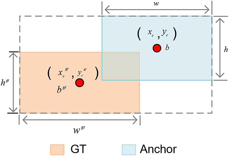
Figure 6: Boundary-box projections

In the above Equation, distanceShape represents the loss component for constraining the accuracy of the bounding box’s center point position. It combines the horizontal and vertical weight coefficients ww and hh. It eliminates the influence of absolute coordinate values via the normalization constant c, allowing the model to focus more on the alignment between the centers of the predicted and ground truth bounding boxes. ΩShape, on the other hand, serves as the loss component for the bounding box’s shape matching accuracy. Quantifying the differences in width and height between the predicted and ground truth bounding boxes drives the model to make the predicted box’s shape more closely resemble the ground truth’s. Therefore, the Shape-IoU bounding box loss not only accounts for the overlap between the ground truth bounding box and the predicted bounding box but also fully considers the deviation in the bounding box’s center point position, as well as its shape and scale characteristics.

NWD is a novel metric for measuring the similarity between predicted and ground bounding boxes. It models them as Gaussian distributions, measures their similarity via Wasserstein distance [30], and normalizes the distance by the ground bounding box scale. By aligning the loss magnitudes of large and small objects, NWD achieves more stable small-object detection performance. The NWD formula is as follows:

B=(w−wgt)2+(h−hgt)2weight2,weight=2(17)

D=hh×(xc−xcgt)2+ww×(yc−ycgt)2+B(18)

NWDShape=e−DC(19)

C is a constant associated with the dataset, which is set to three in this thesis.

The overall size of wind turbine blades is large, while some minor defects are small targets within the image. To enhance the model’s detection of small targets and further improve the accuracy of blade defect identification, the loss function is constructed by combining NWD with Shape-IoU. This approach simultaneously considers both Shape-IoU and NWD within the loss function, assigning reasonable weights to each. The specific calculation formula is as follows:

LNWD−Shape−IoU=0.8×LShape−IoU+0.2×NWDShape(20)

Thus, both Shape-IoU and NWD are considered in the loss function, with reasonable weights assigned to each. Combining Shape-IoU with NWD can more precisely quantify the alignment between the predicted and ground truth boxes, especially for targets with complex shapes, irregularities, or rotations, and provide a finer evaluation. This significantly improves the model’s bounding-box regression precision, resulting in overall performance gains.

3  Dataset

Given the scarcity of publicly available datasets on wind turbine blade defects, this study utilizes a self-constructed dataset. Images were captured using drones at a wind farm in China, ensuring broad coverage of the sample. Geographically, blades from both plains and hilly regions are included, while seasonally, images encompass summer and winter conditions. To enhance the model’s environmental robustness, blade images were specifically collected under rain and snow conditions. The dataset comprises 5029 raw images (resolution 640 × 640), divided into training, validation, and test sets at a 7:2:1 ratio. A total of 702 images were captured under rainy conditions, accounting for approximately 14% of the dataset, while 252 were captured under snowy conditions, representing about 5% of the dataset. Defect annotations categorize six typical defects: lightning strike marks, oil leakage, tape breakage, paint peeling, dirt accumulation, and corrosion. Representative images of each defect category are shown in Fig. 7, while examples of blade images under rainy and snowy conditions are presented in Fig. 8.

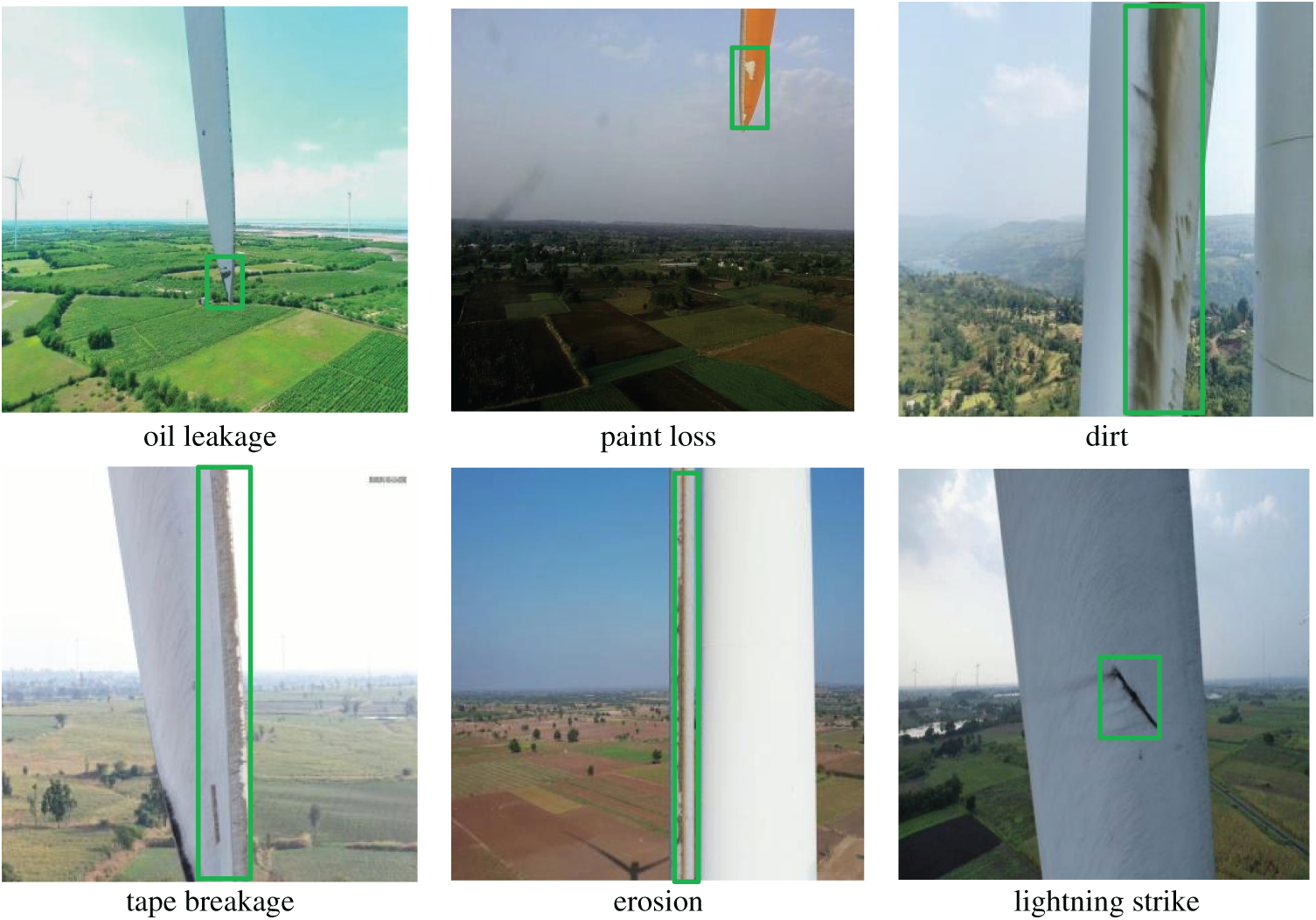
Figure 7: Examples of wind turbine blades and their defects

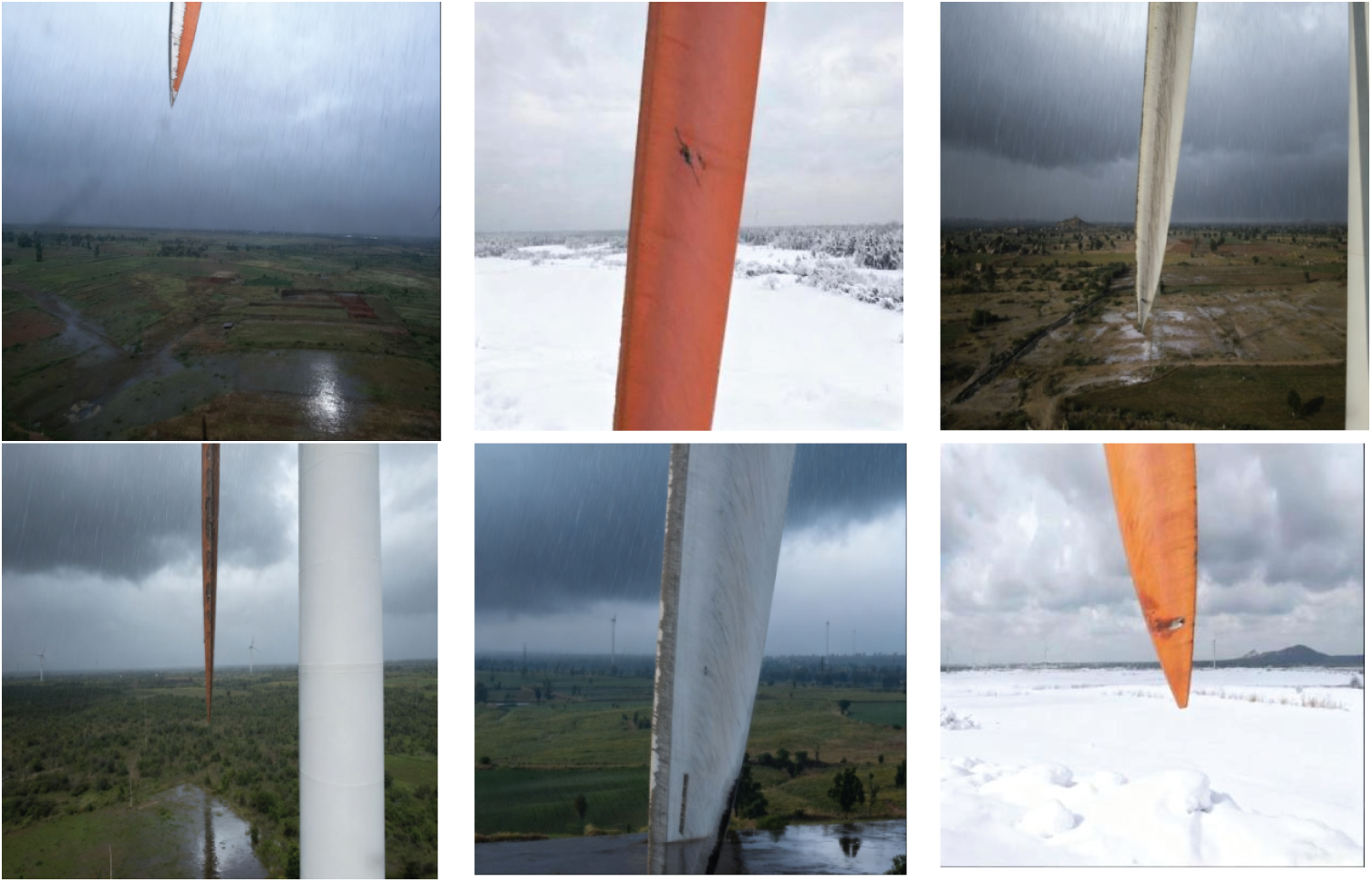
Figure 8: Wind turbine blade images in rainy and snowy weather

Lightning strike defects exhibit sharply defined boundaries accompanied by black burn pits and charred cracks; oil leakage defects appear as continuous black areas with feathered edges and trailing oil streaks; tape breakage sections display mottled colors with exposed substrate, disrupting the color uniformity with surrounding intact tape while rendering the original regular texture discontinuous and rough; dirt defects appear as irregular gray patches with blurred boundary textures; erosion defects often manifest as bulging protrusions. In severe cases, these protrusions may exhibit powdery flaking, appearing in images as uneven, patchy defects. The paint loss defects reveal the base material color of the wind turbine blade, with irregularly shaped contours. The edges may exhibit serrated, jagged, or slightly blurred transition zones.

4  Experiments and Discussions

4.1 Environment and Configuration

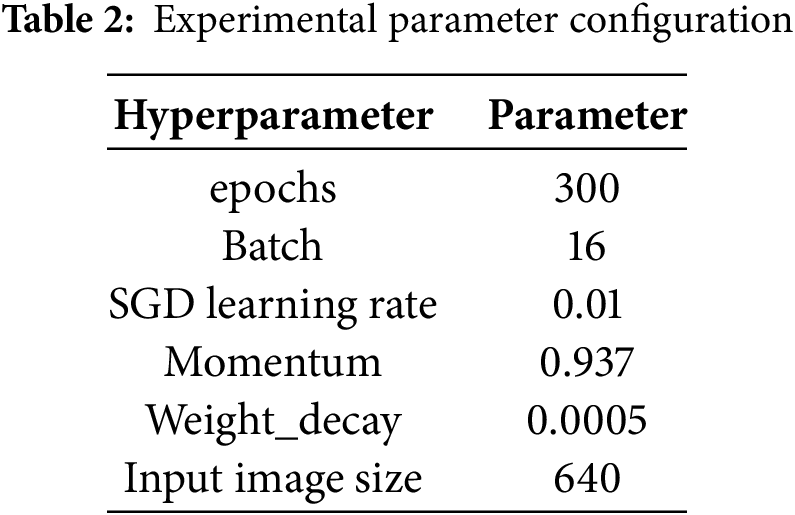
The experimental framework used PyTorch. The experimental platform system was Ubuntu 22.04. The GPU was an RTX 4090D (24 GB), the CPU was a 16 vCPU Intel(R) Xeon(R) Platinum 8474C, PyTorch framework version 2.1.0, Python 3.10 compiler, and CUDA version 12.1. The parameter settings during the experiment are presented in Table 2. The trained model will ultimately be deployed on edge computing devices, specifically the NVIDIA Jetson AGX Orin.

4.2 Experimental Evaluation Indicators

The evaluation metrics used in this thesis include precision (P), recall (R), F1 score, mAP50 for wind turbine blade defect detection, as well as Parameters, GFLOPs, Detection Speed, and Model Size.

Precision is the proportion of all data predicted to be positive samples that are, in fact, positive. For example, the model initially labeled the proportion of samples it predicted as dirty for wind turbine blades as dirty. The formula [31,32] used is as follows:

P=TPTP+FP(21)

here, TP denotes the count of positive samples, whereas FP indicates the number of samples predicted as positive but actually negative.

Recall measures the model’s ability to detect all actual positive instances, defined as the proportion of correctly identified positive samples relative to the total number of actual positives. For example, all wind turbine blade defects are marked as dirty, and the proportion of these that the model correctly detects and classifies as dirty is calculated. The formula [31,32] used is as follows:

R=TPTP+FN(22)

here, FN refers to the number of samples that are positive, but predicted by the model to be negative.

F1 is the reconciled mean of the model in terms of the precision and recall. Precision and recall typically trade off, and the F1 score reflects the model’s combined performance on both. The formula for calculating F1 is as follows:

F1=2×P×RP+R(23)

Average precision (AP) is the average precision of each category, and its value is the area enclosed by the P-R curve and the coordinate axis. The formula [31,32] used is as follows:

AP=∫01P(R)dR(24)

here, P(R) is the precision at the recall rate R.

The mAP averages the AP values across all categories, reflecting the model’s overall accuracy. The larger the mAP value, the more accurate the prediction box. MAP50 refers to the magnitude of the mAP value corresponding to the case in which the IoU threshold is 0.5. The formula [31,32] used is as follows:

mAP=∑i=1kAPik(25)

here, K denotes the number of detected categories, and its value in this experiment is 7.

Params is the number of trainable parameters in the model, reflecting its complexity.

GFLOPs is an essential indicator of a model’s computational complexity. A smaller value indicates that the model requires fewer computational resources from the hardware device during training or inference.

The detection speed is the number of image frames processed per second, a crucial indicator of the model’s real-time and operational capabilities. Wind turbine blade defect recognition applied to UAV equipment has high real-time requirements, and the larger this indicator, the faster the processing speed and the better the real-time performance. This study ultimately selected the NVIDIA Jetson AGX Orin as the edge computing device. Therefore, all detection speed parameters mentioned in the following sections are results from actual runtime testing of the object detection model on this edge device.

Model size refers to the storage space occupied by the model and indicates the hardware resources required during deployment and operation.

4.3 Experimental Results of WtCS-YOLO11 Modeling

The WtCS-YOLO11 model was trained using the developed dataset. The training process loss results are illustrated in Fig. 9, and the performance metrics are depicted in Fig. 10. To better demonstrate its effectiveness, the training result curves of the base model YOLO11n are included in Figs. 9 and 10. The blue curve represents the training result of the base model YOLO11n, and the orange curve represents the training result of the improved model WtCS-YOLO11n. The figure shows that, as iterations increase, the loss values steadily decline and stabilize, while the performance parameters consistently improve and converge. The loss index curves of the WtCS-YOLO11 model are all lower than those of the YOLO11 model, indicating that under identical iteration counts, the loss indexes of the WtCS-YOLO11 model are consistently smaller than those of the YOLO11 model. The WtCS-YOLO11 model’s performance curves consistently outperform those of YOLO11, achieving superior metrics at identical iteration counts and demonstrating greater effectiveness in detecting wind turbine blade defects. The WtCS-YOLO11 model achieved a greater accuracy in detecting wind turbine blade defects.

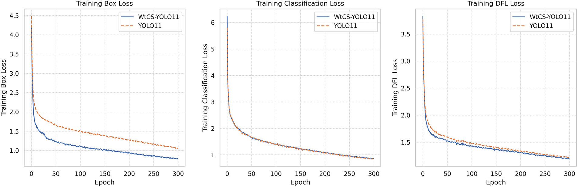
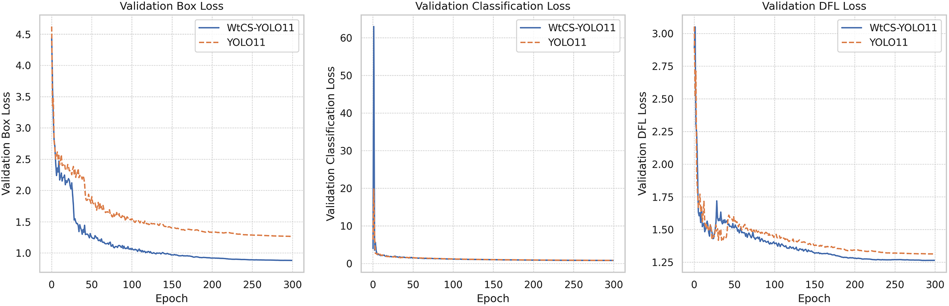
Figure 9: Loss plot of WtCS-YOLO11 model training results

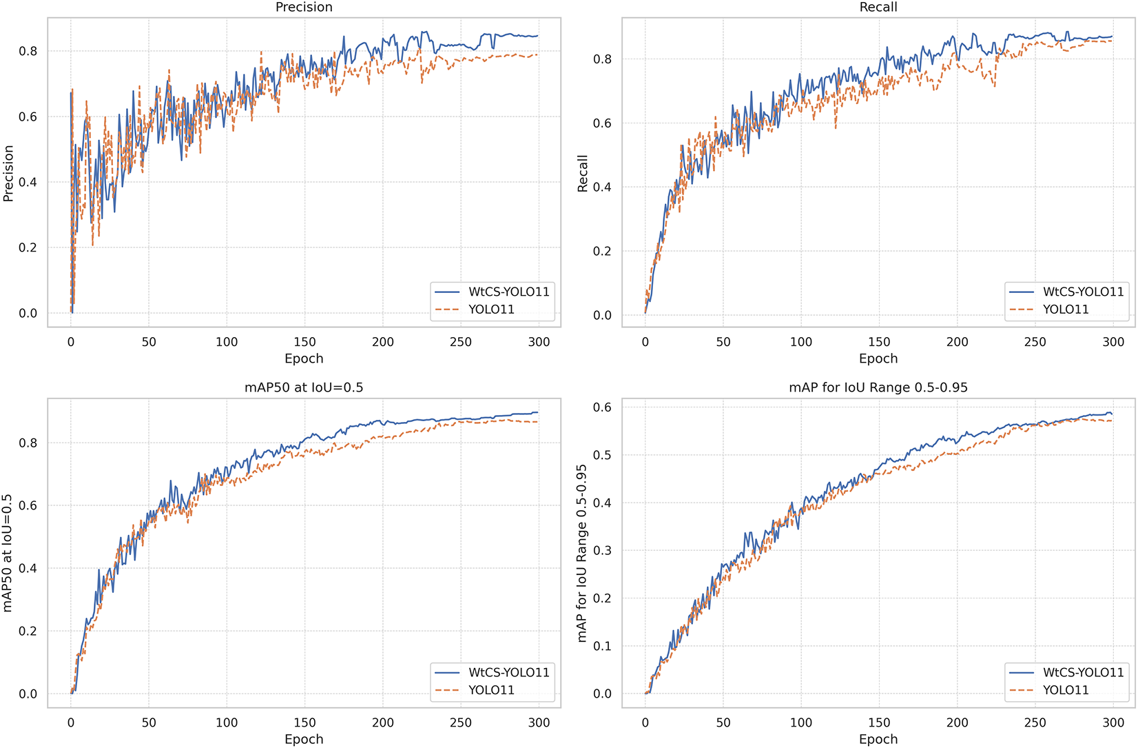
Figure 10: Metrics plot of WtCS-YOLO11 model training results

Fig. 11 shows the precision-recall curve for the WtCS-YOLO11 model, visually illustrating the trade-off between accuracy and recall. The figure reveals that different wind turbine blade defect categories exhibit varying performance in balancing precision and recall. The curve for tape breakage maintains precision near 1.0 across recall values from 0 to 0.8, with only a gradual decline at high recall thresholds. This ensures both high precision and strong recall performance for tape breakage defects, resulting in an AP of 0.995. The curve for oil leakage similarly maintains exceptionally high precision at high recall rates with minimal decline. This reflects outstanding precision alongside high recall in oil leakage defect detection, yielding an AP of 0.967. The curves for lightning strike, erosion, and dirt exhibit a relatively gradual decline in precision as recall increases, maintaining high precision even at medium-to-high recall levels. Consequently, their AP values remain elevated. The curve for the paint loss shows a rapid decline in precision at low recall rates, with overall precision remaining low. This indicates that reducing false negatives for paint loss defects sharply increases false positives, making precision-recall trade-offs more challenging. This results in an AP of only 0.652, indicating that defects like paint loss—characterized by weak features and high background confusion—are more difficult to detect while balancing precision and coverage. Across all categories, the average precision-recall curve shows that precision stabilizes at around 0.897. This indicates that when applied to wind turbine blade defect detection, the model effectively controls false positive rates, accurately identifies defect types, and maintains high recall to prevent missed detections.

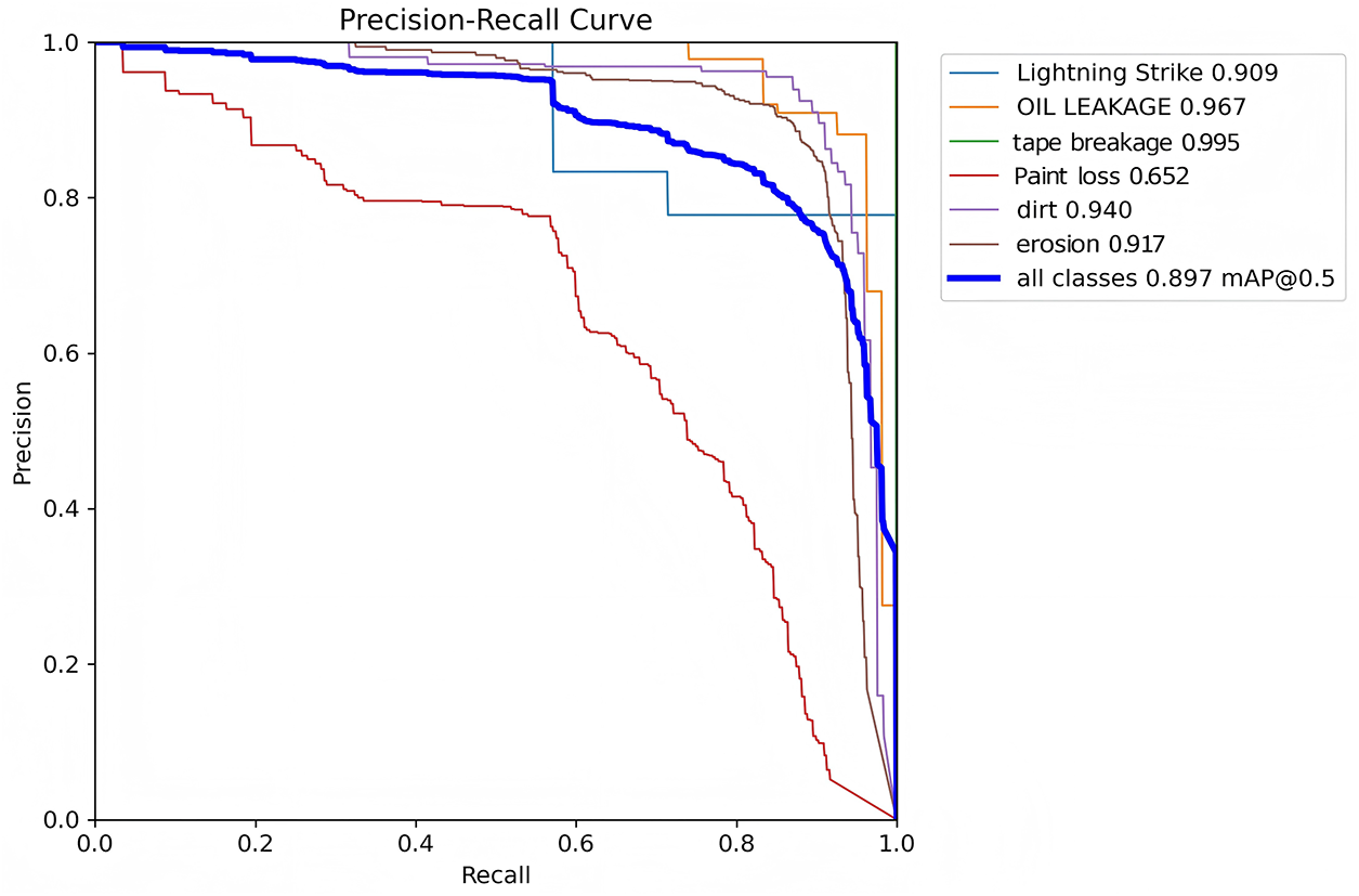
Figure 11: P-R plot of the WtCS-YOLO11 model

Fig. 12 shows the F1-Confidence curves of the WtCS-YOLO11 model, plotting the model’s F1 score at different confidence thresholds. As the confidence threshold changes, the overall change in the remaining curves is relatively smooth, and the model performance changes are more stable under different confidence levels.

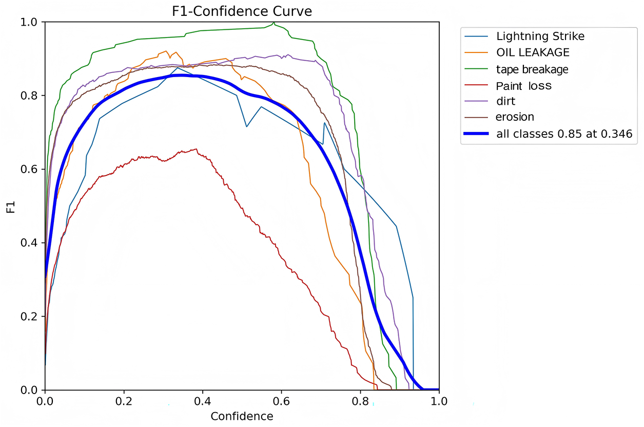
Figure 12: F1-Confidence plot for the WtCS-YOLO11 model

Fig. 13 shows the prediction outcomes of YOLO11 and WtCS-YOLO11. In the first figure, the paint loss defects occupy a small area, which falls under the category of small target detection. The YOLO11 model predicts small targets poorly and fails to detect paint loss as a category. In contrast, WtCS-YOLO11 can effectively recognize the paint loss category. In the second figure, the shape and position of the bounding box predicted by YOLO11 are inaccurate, do not fully cover the area of the paint loss category, and differ significantly from the ground truth bounding box. In contrast, the position and shape of the predicted box of WtCS-YOLO11 are more accurate and are the same as those of the ground-truth bounding box. In the third figure, YOLO11 exhibits both omission and misdetection; the targets of the dirt category are not recognized, and the green plants in the background farmland are incorrectly identified as part of the paint loss category. The WtCS-YOLO11 prediction results effectively avoid this problem.

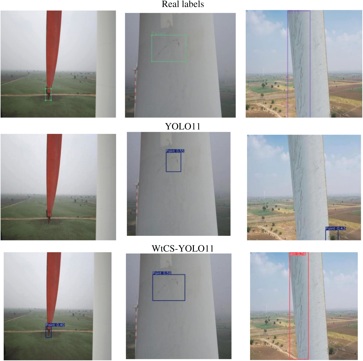
Figure 13: Map of projected results

To evaluate the classification performance of the WtCS-YOLO11 model for six defect categories and background classes in wind turbine blades and to analyze inter-class confusion patterns, a standardized confusion matrix was constructed from the test set, as shown in Fig. 14. Matrix elements reflect classification assignment ratios, where the diagonal represents the correct classification rate and off-diagonal elements represent the misclassification rate between classes. Regarding correct classification rates, both tape breakage and lightning strike achieved 100% accuracy. The former is easily identified by its distinct block-shaped missing edges, while the latter is recognized by its unique linear crack features. Oil leakage reached 96% accuracy. Dark oil stains form high-contrast soaked areas on light-colored blade surfaces, enhancing detectability. Dirt scored 93%, with clustered textures distinctly different from surrounding areas; erosion reached 90%, where irregular rough textures remained distinguishable despite low-light interference; paint loss recorded only 65%—the lowest among all categories—due to its minute size, blurred edges, and low contrast with the background, making it difficult for the model to extract differentiating information; Background features show 26% misclassified as paint loss, 5% as dirt, and 7% as erosion. This occurs because background elements, such as light-colored mottling on leaf surfaces, resemble the characteristics of defects. Regarding cross-class misclassification: Paint loss and dirt exhibit bidirectional confusion, with 18% of paint loss misclassified as dirt and 11% of dirt misclassified as paint loss, due to high overlap in light-colored coverage areas and texture details; Erosion was misclassified as dirt in 9% of cases, as its coarse texture under low-light conditions easily mimics the clustered patterns of dirt. Oil leakage was misclassified as erosion in 6% of cases because it resembled localized texture anomalies commonly associated with erosion. Lightning strike defects were misclassified as tape breakage in only 2% of cases, although both exhibit linear features; the impact is minimal. Overall, the model demonstrates high classification accuracy for defects with distinct features but struggles with ambiguous, easily confused cases of paint loss, often misclassifying backgrounds as paint loss. Future improvements should focus on expanding paint loss sample sets, incorporating low-contrast feature enhancement modules for small-scale details, and optimizing lighting-adaptation processing to enhance model performance.

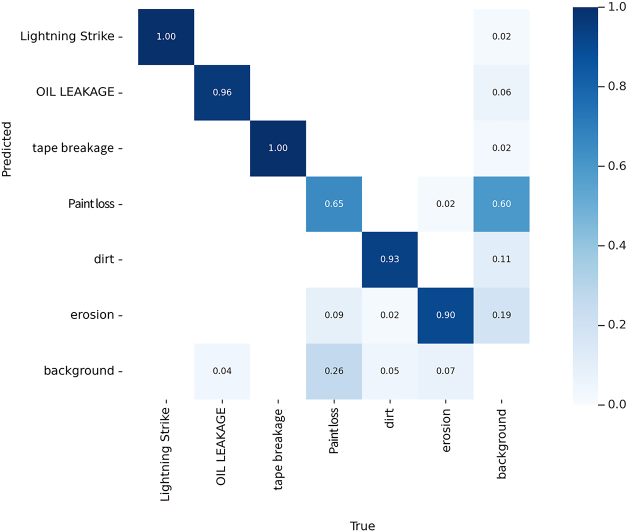
Figure 14: Defect category confusion matrix

4.4 Ablation Experiments

To evaluate the effectiveness of each module in detecting wind turbine blade defects, ablation experiments were conducted on a dataset of blade defects constructed for this purpose. The original YOLOv11n served as the baseline model. The C3k2_WTConv, CBAM, and NWD-Shape-IoU modules, along with their various combinations, were successively integrated into the model. Each experiment employed the identical dataset and hyperparameter settings, with the random seed fixed at 42. Each experimental configuration was independently replicated three times to ensure the stability and reliability of the results. The results of the ablation experiments are presented in Table 3.

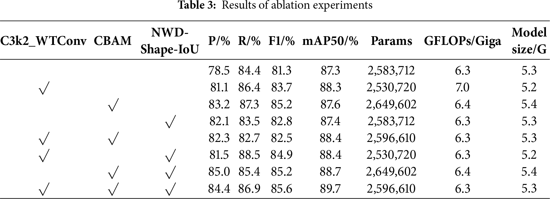
Incorporating the C3k2_WTConv module into the YOLO11 model led to a 2.6% increase in precision, 2.0% increase in recall, 2.4% increase in F1 score, and 1.0% enhancement in mAP50. A reduction in the number of parameters accompanied a performance improvement. Similarly, comparing the data of YOLO11+CBAM+NWD-Shape-IoU and YOLO11+CBAM+NWD-Shape-IoU+C3k2_WTConv, there was a 1.5% boost in recall, a 0.4% rise in F1 score, and a 1.0% enhancement in mAP50. A decrease in the number of parameters by 52,992 and a reduction of the number of GFLOPs by 0.1 Giga. It can be seen that C3k2_WTConv’s wavelet-domain convolutional method covers a larger region of the original image, thereby increasing the receptive field and enhancing the effectiveness of wind turbine blade defect detection. A small convolution kernel size decreased the model’s parameter count.

By comparing the data in the first and third rows of Table 3, the addition of the CBAM module to the YOLO11 model resulted in a 4.7% increase in precision, a 2.9% increase in recall, a 3.9% increase in F1, and a 0.3% increase in mAP50. Despite a rise in parameter count, the increase was only 65,890, which remains within an acceptable range and does not hinder the model’s deployment on edge devices. Similarly, comparing the data from YOLO11+C3k2_WTConv+NWD-Shape-IoU and YOLO11+C3k2_WTConv+NWD-Shape-IoU+CBAM, there was an increase of 2.9% in accuracy, 0.7% in F1, and 1.3% in mAP50. It can be seen that the CBAM module introduces spatial attention and channel attention, reasonably adjusting the feature weight of each channel and spatial location in the feature map. This enables the model to automatically allocate attention to different regions, thereby facilitating the detection of significant defects in wind turbine blades. The accuracy of wind turbine blade defect detection was improved based on a slight increase in the number of parameters and model complexity.

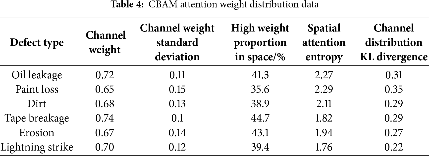
Table 4 presents quantitative data on the distributions of channel and spatial attention weights under different wind turbine blade defect types, utilizing the CBAM attention mechanism. The channel mean weight reflects the average attention level across defect-feature channels, while the channel-weight standard deviation indicates the dispersion of attention allocation among channels. The spatial high-weight proportion represents the percentage of defect regions receiving high attention in the spatial dimension, and spatial attention entropy measures the disorder in spatial attention distribution. Where lower entropy indicates more concentrated attention. The Kullback-Leible (KL) divergence of the channel distribution measures the difference between the channel attention distribution and the baseline distribution, with lower values indicating greater distributional matching. These multidimensional metrics intuitively reveal CBAM’s differential attention allocation across channels and spatial dimensions for distinct defect types. This demonstrates CBAM’s capability to dynamically optimize attention strategies based on visual feature differences—such as lightning strike, oil leakage, and tape breakage—making it adaptable for multi-defect detection tasks on wind turbine blades.

Replacing the NWD-Shape-IoU module in the YOLO11 model resulted in a 3.6% increase in accuracy, a 1.5% increase in F1 score, a 0.1% increase in mAP50, and no change in the number of parameters or GFLOPs. Similarly, comparing the data of YOLO11+CBAM+C3k2_WTConv and YOLO11+CBAM+C3k2_WTConv+NWD-Shape-IoU, the precision was improved by 2.1%, the recall was improved by 4.2%, F1 was improved by 3.1%, the mAP50 was improved by 1.3%, and the number of parameters and GFLOPs did not change. It can be observed that Shape-IoU combined with NWD can more accurately reflect the actual degree of similarity between the predicted frame and the absolute frame and can provide a finer assessment when identifying complex and irregular shape defects in wind turbine blades, which improves the precision of defect detection in wind turbine blades without increasing the model complexity and model size.

4.5 Comparative Experiment

4.5.1 Comparison Experiment of C3k2 Convolution Modules

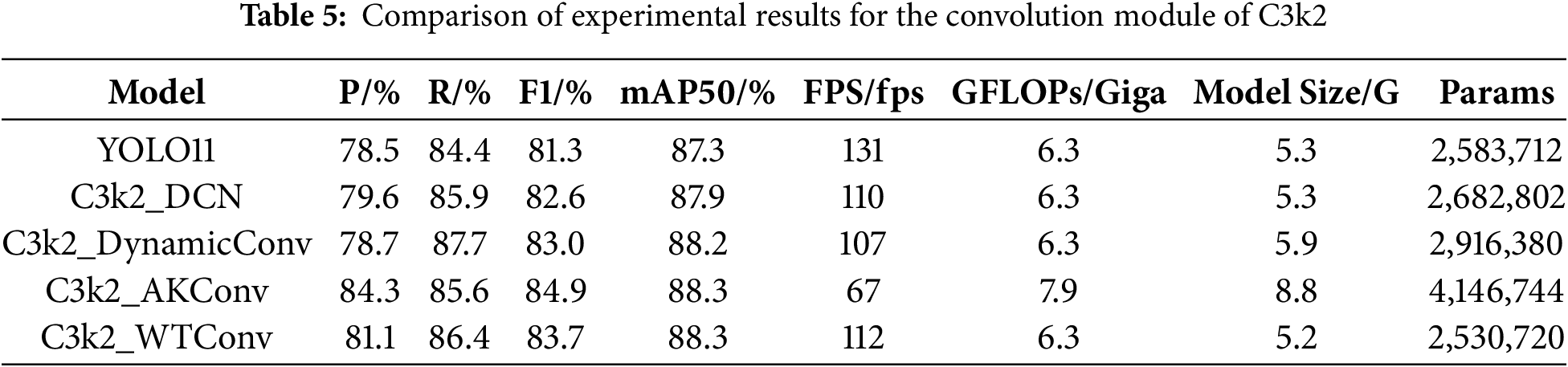
Improvements were made to the convolutional module in C3k2. As shown in Table 5, using the cross-stage partial with two kernels and a deformable convolution module (C3k2_DCN) to improve the original YOLO11 model resulted in a 0.4% increase in mAP50, a 1.3% increase in F1 score, an increase of 99,090 parameters, and a decrease of 21 frames per second in detection speed (FPS). The C3k2_DCN module maintains a slight improvement in accuracy. After improving the model using the cross-stage partial with two kernels and a dynamic convolution module (C3k2_DynamicConv), mAP50 increased by 0.9%, F1 score increased by 2.3%, the number of parameters increased by 332,668, the model size increased by 0.4 GB, and the detection speed decreased by 24 frames per second (fps). Although the C3k2_DynamicConv module improves detection accuracy, the increase in parameter count and model size makes it unsuitable for deployment on resource-constrained devices such as drones. After enhancing the model using the cross-stage partial with two kernels and an adaptive kernel convolution module (C3k2_AKConv), mAP50 increased by 1%, F1 increased by 3.4%, but the number of parameters increased by 1,563,032, the model size increased by 3.5 MB, GFLOPs increased by 1.6 Giga, and the detection speed decreased by 64 frames per second. Although the C3k2_AKConv module performed well in terms of detection accuracy and F1 score, the significant decrease in FPS makes it challenging to meet the real-time detection requirements for drone devices. After using the C3k2_WTConv module for improvement, mAP50 increased by 1%, F1 score increased by 2.4%, the number of parameters decreased by 52,992, the model size decreased by 0.1 MB, and FPS decreased by 19 fps. The C3k2_WTConv module improves detection accuracy while reducing the number of model parameters and model size. Although the detection speed decreases, it does not affect real-time detection on drones. Comparison experiments demonstrate that the C3k2_WTConv module achieves superior performance and is better suited for defect detection in wind turbine blades.

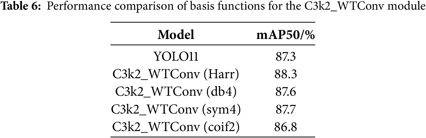
To further validate the underlying mechanisms and performance differences among various wavelet basis functions in model detection, this study adopted YOLO11 as the baseline model. By incorporating the C3k2_WTConv module, four distinct wavelet basis functions—Haar, db4, sym4, and coif2—were sequentially introduced to enhance the results. The detection accuracy results for each model are presented in Table 6. The baseline YOLO11 model achieved an mAP50 of 87.3%, while the C3k2_WTConv model employing Haar wavelet basis functions achieved 88.3%. Fully demonstrating the Haar wavelet’s significant advantage in capturing high-frequency defect features such as tape damage and lightning strikes due to its shortest support length, highest temporal resolution, and excellent high-frequency response sensitivity, thereby effectively improving model detection accuracy. The C3k2_WTConv module model using db4 wavelet basis functions achieved an mAP50 of 87.6%, while the same module model with sym4 wavelet basis functions reached 87.7%. Although db4 offers certain advantages for extracting low- to mid-frequency defects, its high-frequency response decays rapidly. Sym4, while exhibiting lower phase distortion than db4, still suffers from noticeable energy loss in the high-frequency band. The C3k2_WTConv module with the coif2 wavelet basis achieved an mAP50 of 86.8%. The coif2 wavelet basis function exhibits nearly complete attenuation at high frequencies, rendering it ineffective at capturing core high-frequency defects, such as tape damage and lightning strikes. The aforementioned experimental results further validate the adaptability advantages of Haar wavelet bases in wind turbine blade defect detection scenarios and provide data-driven support for wavelet basis function selection.

4.5.2 Attention Mechanism Comparison Experiment

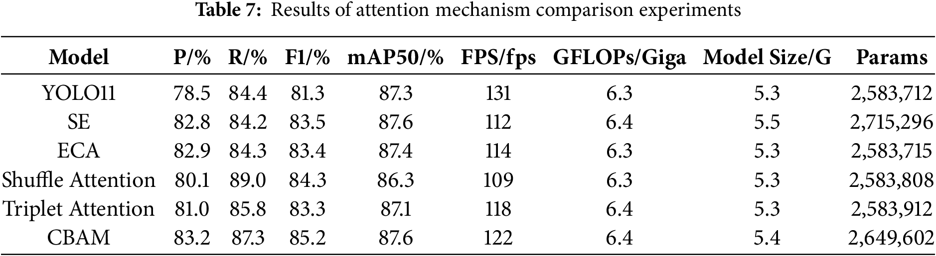
To validate the superiority of the CBAM attention mechanism, comparisons were made with mainstream attention mechanisms, including Squeeze-and-Excitation Attention (SE), ECA, Shuffle Attention, and Triplet Attention. The experimental results are presented in Table 7. Compared to the baseline model, adding the SE attention mechanism increased mAP50 by 0.3%, F1 by 2.4%, the number of parameters by 131,584, and GFLOPs by 0.1 Giga, while reducing FPS by 19 fps. Although detection performance was improved, the increases in the number of parameters and computational complexity made it difficult to effectively balance detection performance and model complexity, which is unfavorable for deployment on resource-constrained devices such as drones. After adding the ECA mechanism, mAP50 increased by only 0.1%, F1 by 2.1%, and the number of parameters, GFLOPs, and model size remained almost unchanged compared to the baseline. The ECA mechanism shows limited improvement in the model’s detection performance. After adding the Shuffle Attention and Triplet Attention mechanisms, mAP50 decreased, indicating that these two modules do not improve the detection of wind turbine blade defects. After adding the CBAM module, mAP50 increased by 0.3%, F1 score by 3.9%, the number of parameters by 65,890, and GFLOPs by 0.1 Giga, while FPS decreased by 9 frames per second. Overall, the addition of the CBAM attention mechanism yielded the most tremendous improvement in detection accuracy. The relatively minor increases in the number of parameters and computational complexity are within acceptable limits. Although FPS decreased slightly, it does not affect real-time detection on uncrewed aerial vehicles.

To clearly illustrate the attention tendencies of different mechanisms toward features, this study visualized their operational results using heatmaps. The heatmaps utilize varying shades of color to represent the model’s attention intensity toward other regions. Warm tones, such as red, orange, and yellow, indicate a higher probability of the target being present in that area. In contrast, cool tones, including blue, green, and cyan, indicate a lower likelihood. As shown in Fig. 15, YOLO11 and ECA not only form warm-toned focal spots in target regions but also exhibit additional attention to non-defective areas of turbine blades, which may lead to misclassifications. This phenomenon will increase the risk of false positives in defect detection tasks and further undermine the model’s reliability. Shuffle Attention displays warm tones that are widely distributed across both the background and target regions, indicating overly dispersed attention that is susceptible to interference from non-oil-leakage areas. This dispersion also causes the model to waste computational resources on irrelevant regions, which reduces its inference speed. Triplet Attention exhibits a scattered, warm-toned distribution, with insufficient focus on oil-leakage areas and insufficient concentration, making it difficult to capture the core leakage zones accurately. This limitation becomes more critical when dealing with minor or irregularly shaped leakage spots, as these targets require precise localization from the model. CBAM generates clear, concentrated warm-toned spots in oil-leakage areas, with the background almost entirely composed of cool tones. This indicates a strong focus on leakage zones and an optimal background suppression capability, effectively highlighting target regions. Such performance advantages make CBAM more suitable for real-world industrial applications, such as turbine blade maintenance, where both accuracy and efficiency are of great importance.

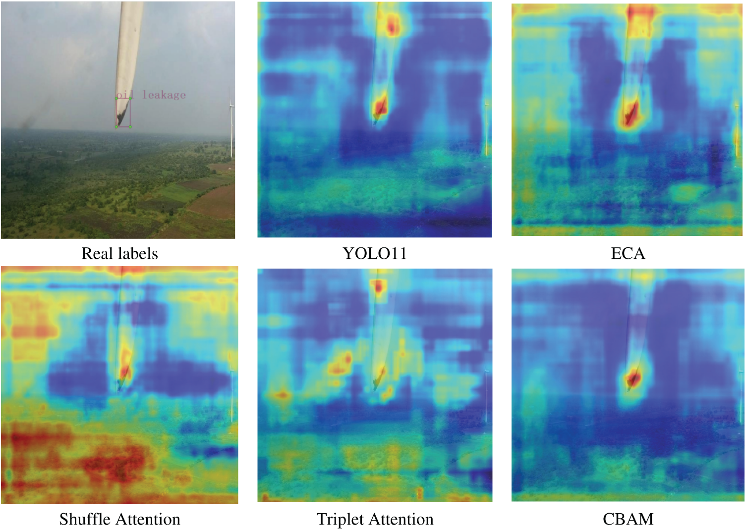
Figure 15: Differences in feature extraction via attention mechanisms

4.5.3 Bounding Box Loss Function IoU Comparison Experiment

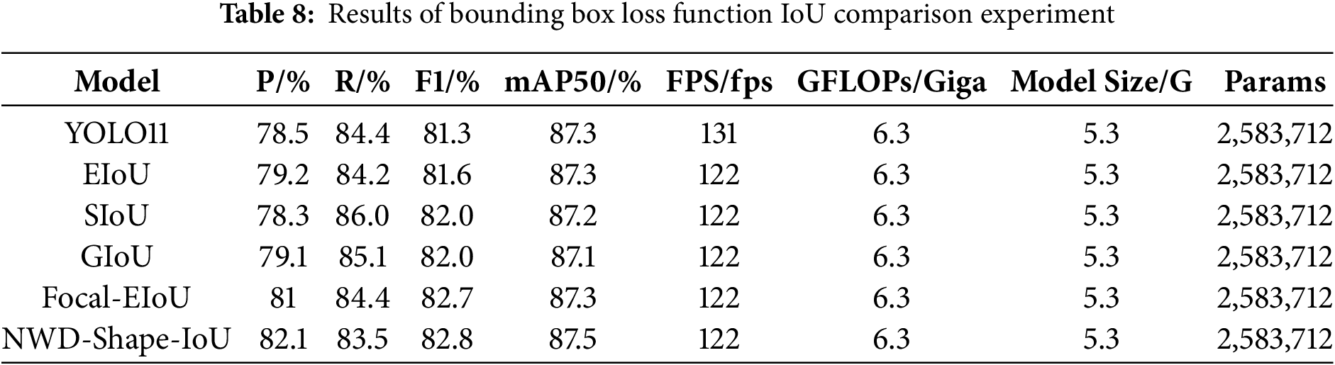
To validate the effectiveness of the proposed NWD-Shape-IoU, it was compared and analyzed with mainstream loss functions. The baseline YOLO11 model used generalized intersection over union (GIoU). As shown in Table 8. When the baseline model was improved to enhance intersection over union (EIoU), mAP50 did not improve, while the F1 score increased by 0.3%, suggesting that EIoU had a limited impact on detection performance. When the baseline was improved to scaled intersection over union (SIoU), although F1 increased by 0.7%, mAP50 decreased by 0.1%, suggesting SIoU was not adequate for this specific task. Similarly, when adopting GIoU, F1 increased by 0.7%, but mAP50 dropped by 0.2%, rendering GIoU unsuitable for wind turbine blade defect detection. After replacing the loss function with Focal-EIoU, F1 increased by 1.4%, while mAP50 remained unchanged. In contrast, implementing NWD-Shape-IoU resulted in a 1.5% increase in F1 and a 0.2% increase in mAP50. In addition to the above experiments, we also investigated the detection performance of NWD-Shape-IoU across different scales. The results demonstrate that NWD-Shape-IoU achieves stable improvements across all size ranges, particularly in detecting small-scale defects. Overall, NWD-Shape-IoU shows the most significant improvement in detection performance and is better suited for wind turbine blade defect detection.

4.5.4 Comparative Experiments between WtCS-YOLO11 and Other Models

To compare the performance of the improved model with that of the other models, we conducted comparison experiments on this dataset. The hyperparameter settings remained constant throughout the experiments, and the experimental outcomes are presented in Table 9.

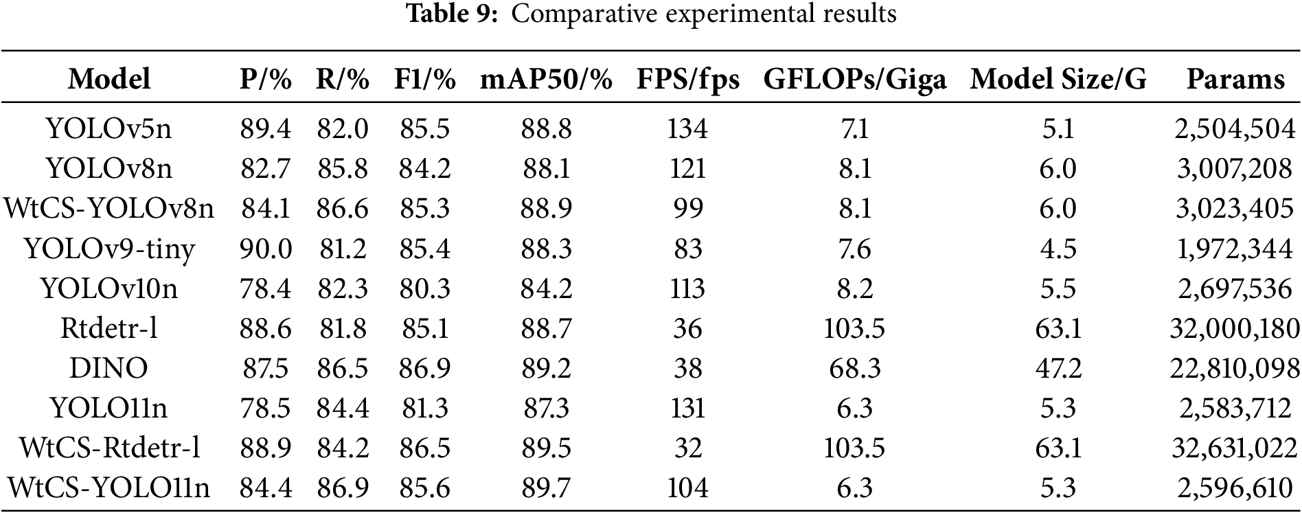
As shown in Table 9, the improved model WtCS-YOLO11n achieved a 5.9% increase in precision, a 2.5% increase in recall, a 4.3% increase in F1 score, and a 2.4% increase in mAP50 compared to the base model YOLO11n. The GFLOPs and model size remained unchanged, while the number of parameters increased slightly, by 12,898. Although the number of parameters increased, it is not crucial and does not affect the model’s application to UAV edge devices. The improved model is more accurate and comprehensive for detecting wind turbine blade defects, and its performance is significantly enhanced.

You Only Look Once Version 9 Tiny (YOLOv9-tiny) achieves the highest model precision of 90.0%, occupying the smallest storage space and requiring the fewest parameters while maintaining the best lightweight performance. However, the recall is poor, only 81.2%, and the most important index, mAP50, is lower than that of WtCS-YOLO11n. The model’s FPS is low, the detection process is inefficient, and its real-time capabilities are suboptimal. The mAP50 of WtCS-YOLO11n is the highest, much higher than that of the other models, and the model performs best in terms of recall and GFLOPs. This indicates that WtCS-YOLO11n has a better detection performance for wind turbine blade defects. The You Only Look Once Version 5 Nano (YOLOv5n) model achieves the highest FPS and the fastest image processing speed; however, it does not perform well on other parameter metrics.

Both Real-Time Detection Transformer-Large (Rtdetr-l) and DINO are Transformer-based detection models. As shown in the Table 9, DINO demonstrates higher mAP50 and F1 scores while being more compact in terms of model parameters and size than Rtdetr-l. While also achieving slightly higher FPS than Rtdetr-l. However, both models still exhibit relatively high GFLOPs requirements, and their FPS values remain significantly lower than those of the WtCS-YOLO11n model. Furthermore, on the mAP50 metric, WtCS-YOLO11n outperforms DINO with 89.7%, while also demonstrating balanced performance across recall and F1 score. Overall, while Transformer-based models excel in specific metrics, WtCS-YOLO11n achieves the highest mAP50 score while maintaining high detection speed. Its smaller model size and parameter count make it more suitable for drone edge devices, delivering superior overall performance in wind turbine blade defect detection tasks.

The results of WTConv-CBAM-Shape-IoU-You Only Look Once Version 8 Nano (WtCS-YOLOv8n) demonstrate that, after implementing the proposed improvement scheme, the model’s accuracy, recall, F1 score, and mAP50 all improve compared to the original You Only Look Once Version 8 Nano (YOLOv8n). This indicates that the scheme is effective and exhibits strong generalization, thereby significantly enhancing the model’s detection performance. We further applied the innovations proposed in this paper to the Rtdetr model and conducted comparative experiments. Compared with the original Rtdetr-l model, the WTConv-CBAM-Shape-IoU-Real-Time Detection Transformer-Large (WtCS-Rtdetr-l) model achieved a 0.3% improvement in precision, a 2.4% increase in recall, an absolute 1.4 gain in F1-score, and a 0.8% improvement in mAP50. Notably, these performance gains are achieved without altering the model’s GFLOPs or size; only the number of parameters increased slightly. This confirms that the innovative method proposed in this paper can be effectively adapted to other model architectures and exhibits strong generalization ability.

As shown in Fig. 16, which comprehensively reflects the performance of all models across all parameter indicators, WtCS-YOLO11n has the most extensive coverage area and superior overall performance. In addition to achieving the best performance in mAP50, R value, and GFLOPs, the performance of the other parameter indicators is also impressive, with no abnormal performance across any of them. Although the FPS value is not outstanding for wind turbine blade defect detection, the number of target types to be recognized is not significant. To ensure recognition accuracy, the FPS value of the real-time detection model applied to UAVs between 60 and 90 can satisfy the detection requirements. The FPS of WtCS-YOLO11 reached 104, which was more than sufficient to meet the real-time detection requirements of UAVs. Therefore, WtCS-YOLO11 is highly suitable for implementation on edge devices or embedded systems, while maintaining a high recognition performance. The prediction rate is sufficiently high to meet the demands of real-time detection, making it suitable for UAVs to identify defect types on wind turbine blades.

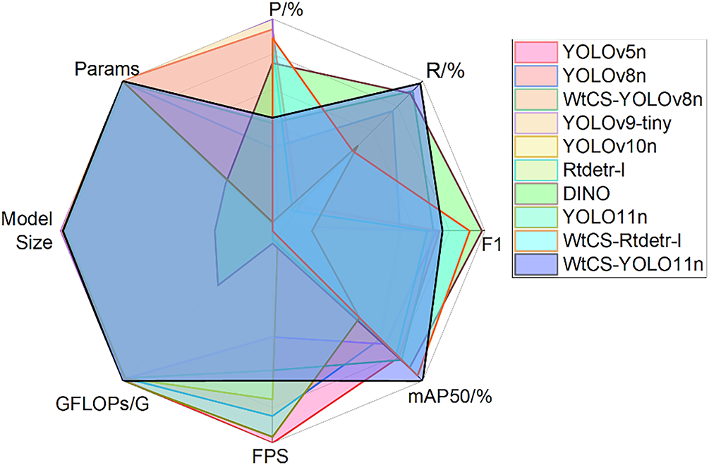
Figure 16: Comparison of the comprehensive performance of each model

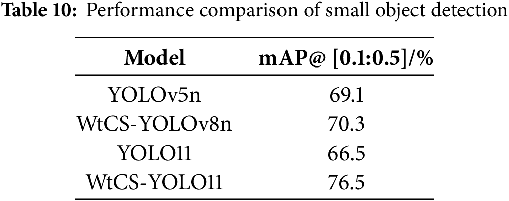
During drone-based inspections of wind turbine blades, factors such as high-altitude shooting angles, defect dimensions, and surface texture interference can introduce small-target defects, including narrow paint loss, minor tape breakage, and localized dirt. Accurate detection of these defects is critical for ensuring blade integrity assessment. To further validate the WtCS-YOLO11 model’s detection advantages for small-target defects, this study selected 106 representative small-target defect samples from the wind turbine blade defect test dataset constructed in the paper. Models with relatively good performance in Table 9, such as YOLOv5n, WtCS-YOLOv8n, and YOLO11n, show strong performance from the paper’s test dataset. The comparison focused on the small object detection metric mAP@ [0.1:0.5], with results shown in Table 10. The table clearly indicates that WtCS-YOLO11 achieves a mAP@ [0.1:0.5] of 76.5% for small object detection, representing a 10 percentage point improvement over the baseline YOLO11n model, a 6.2 percentage point gain over WtCS-YOLOv8n, and a significant advantage over YOLOv5n. This performance edge stems from the triple enhancements proposed in the paper: the C3k2_WTConv module captures high-frequency edge details of small objects through wavelet decomposition; CBAM attention suppresses background interference to focus on small-object regions; and NWD-Shape-IoU optimizes the accuracy of small-object bounding-box regression. These three components synergistically achieve targeted performance improvements in small object detection.

4.6 Comparison of Test Results under Different Weather Conditions

To validate the model’s environmental robustness, the original test dataset was divided into two categories: clear-weather samples and adverse-weather samples. The clear-weather samples comprised 352 images, accounting for 70% of the test set. These covered sunny illumination conditions in both plains and hilly regions, with leaf surfaces free of precipitation interference, precise defect edges, and high feature recognition accuracy. The adverse weather samples comprised 151 images, accounting for 30% of the test set. These included naturally captured images from rainy and snowy days, showcasing phenomena such as rainwater reflections on leaf surfaces, light snowfall, and blurred defect edges. The test results are presented in Table 11.

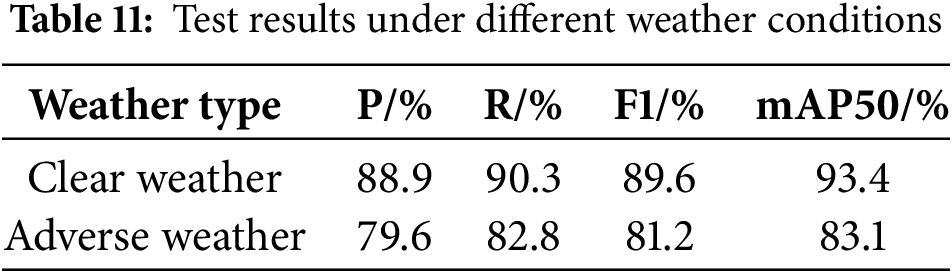
As shown in Table 11, under various weather conditions, the WtCS-YOLO model achieved a precision of 88.9%, a recall of 9 0.3%, and an F1 score of 89.6% in clear weather, with mAP50 of 93.4%. All metrics demonstrate excellent performance, fully showcasing the model’s precise detection and efficient recall capabilities for wind turbine blade defects in ideal scenarios where defect features are clear and precipitation interference is minimal. Under adverse weather conditions, including rain and snow, despite blade surface defects exhibiting blurred edges and reduced feature recognition due to factors like rainwater reflection and thin snow coverage, the model maintained high performance with precision at 79.6%, recall at 82.8%, F1 score at 81.2%, and mAP50 at 83.1%, indicating a controlled performance degradation. This outcome demonstrates that the WtCS-YOLO model achieves reliable defect detection even in complex precipitation scenarios, exhibiting strong environmental robustness and adaptability to the variable outdoor weather conditions encountered during wind turbine inspections.

4.7 Error Analysis of the WtCS-YOLO 11 Model

Although the WtCS-YOLO11 model has achieved significant progress, false positives and false negatives still occur in defect detection on wind turbine blades. Table 12 summarizes the misdetection and missed detection rates for each defect type during testing. Paint loss defects had the highest false-negative rate among all defect types at 22.5% and also exhibited a relatively high false-positive rate of 19.9%. This indicates that, due to their characteristics—small size, blurred edges, and tendency to blend with the background—paint loss defects are both underdetected and misclassified as non-defective areas. Lightning strike defects had the highest false positive rate at 20.1%. This is primarily because lightning strike defects typically manifest as minute local damage on blade surfaces. Their small scale and subtle visual characteristics make it difficult for models to accurately distinguish genuine defects from inherent blade textures or stains against complex backgrounds. Tape breakage defects exhibit distinct characteristics with precise contours, yielding the best performance with a false-negative rate of 4.3% and a false-positive rate of 6.7%. The false-negative and false-positive rates for erosion, dirt, and oil leakage are relatively moderate. These discrepancies indicate that the WtCS-YOLO11 model still has room for improvement when addressing small targets, low-contrast defects, and defects that closely resemble the background or their own textures.

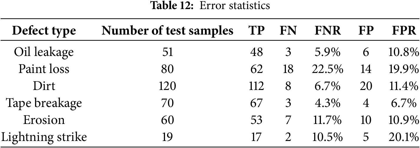
Fig. 17 illustrates typical false positives and false negatives encountered during testing. In the first image, the dim lighting conditions made the farmland appear similar to the oil spill area. While the model detected the oil spill, it produced redundant annotations and mistakenly identified the shadow of a wind turbine blade as a lightning strike defect. In the second image, the area of paint loss was extremely narrow, and the model failed to detect it entirely. In the third image, the area struck by the lightning is small, and the camera was positioned far away during capture, resulting in extremely faint crack features characteristic of lightning damage. The model incorrectly classified this as paint loss, both missing the actual lightning defect and misclassifying the paint loss category. This highlights the challenges small targets and low feature saliency pose to model recognition. These cases demonstrate that future research must optimize the model across multiple dimensions: exploring more suitable confidence thresholds to balance detection accuracy and recall; expanding datasets to cover complex scenarios like low-light conditions, small objects, and long-distance photography; and specifically enhancing the model’s ability to identify defects in small objects and those with similar visual characteristics. These efforts will further improve detection accuracy.

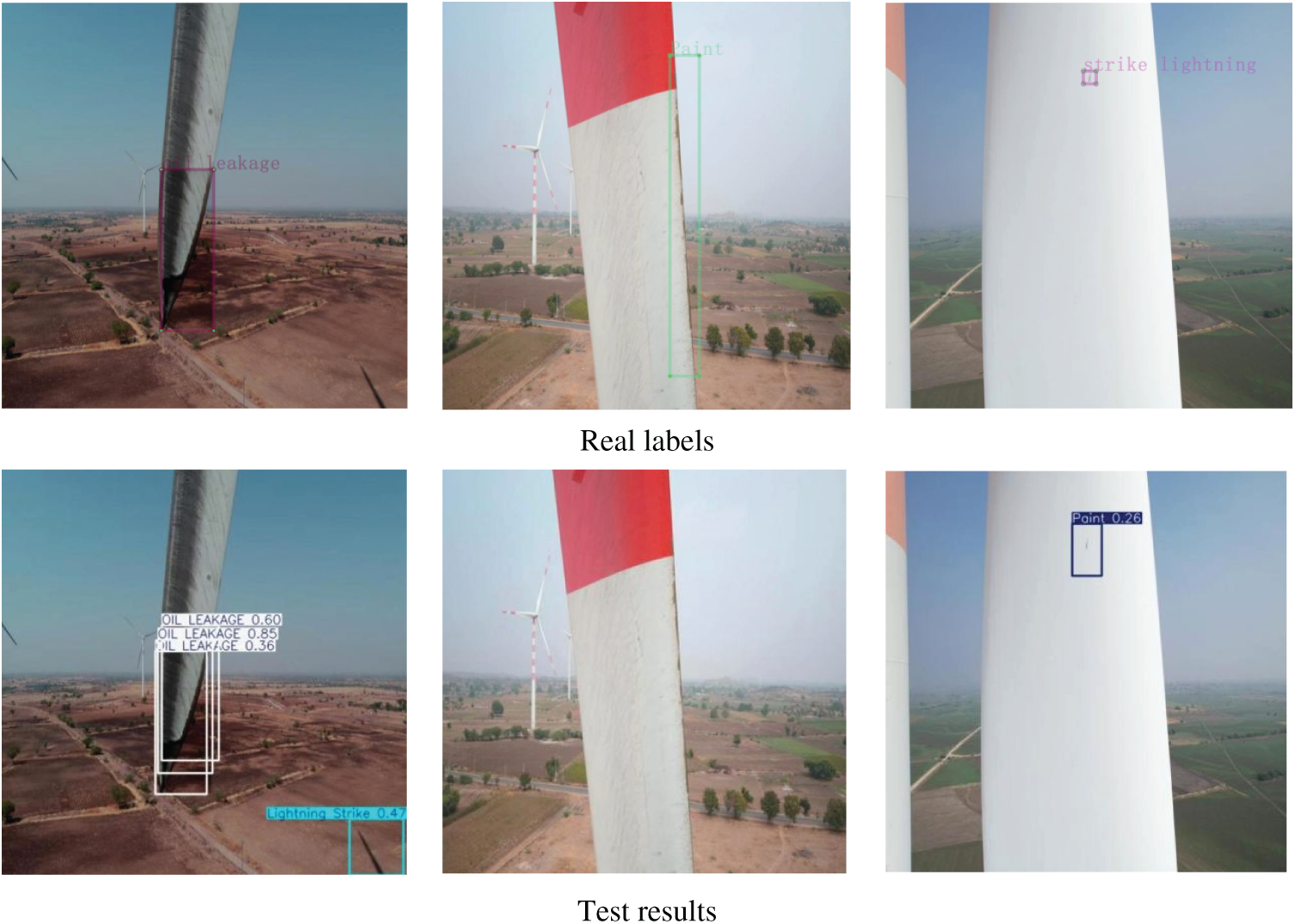
Figure 17: False positive and false negative cases

4.8 Model Deployment

NVIDIA Jetson AGX Orin is a high-end embedded platform explicitly designed for edge computing. It delivers up to 85 trillion floating-point operations per second (TFLOPS) of 16-bit floating-point (FP16) performance and 275 trillion operations per second (TOPs) of 8-bit integer (INT8) performance, featuring high-performance CPU and GPU capabilities paired with 64 GB of low-power double data rate 5 SDRAM (LPDDR5) memory. It supports multi-sensor data fusion and real-time AI inference. The Jetson TX2 was once the mainstream mid-range embedded platform, delivering 1.3 TOPs of INT8 performance with 8 GB of memory. It requires tools like TensorRT for adapting modern Artificial Intelligence (AI) models. The Jetson Nano is a cost-effective embedded platform for entry-level scenarios. After TensorRT quantization, its INT8 performance reaches approximately 0.236 TOPs. Equipped with 4 GB of memory and featuring ultra-low power consumption of 5–10 W, it is primarily used in education, lightweight visual inspection, and IoT devices.

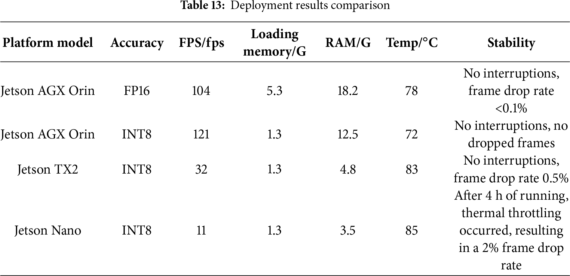
Table 13 presents deployment data for the WtCS-YOLO11 model across three embedded platforms. NVIDIA Jetson AGX Orin demonstrates outstanding performance, supporting both FP16 and INT8 double-precision deployments. FP16 preserves the model’s floating-point parameters, while INT8 uses quantization to convert floating-point values to INT8 integers. Although this reduces model storage requirements, it results in a slight decrease in detection performance. Regarding peak temperature and continuous operation stability metrics, the Jetson AGX Orin achieves a peak temperature of 78°C when running in FP16 format, maintaining uninterrupted operation with a frame drop rate <0.1%. When operating in INT8 format, the peak temperature decreases further to 72°C, allowing for uninterrupted operation without frame drops and demonstrating superior thermal performance and continuous stability. Limited by their memory capacity, Jetson TX2 and Jetson Nano only support deployment in INT8 quantization format. The Jetson TX2 reached a peak operating temperature of 83°C, maintaining continuous operation without interruption, but exhibited a 0.5% frame drop rate. The Jetson Nano reached a peak operating temperature of 85°C. After 4 h of operation, thermal throttling occurred, resulting in a 2% frame drop rate and suboptimal stability of continuous operation. Testing demonstrated that the NVIDIA Jetson AGX Orin platform achieved a maximum frame rate of 104 FPS in FP16 mode, meeting real-time detection requirements for drones. While the Jetson TX2 and Jetson Nano platforms exhibit lower detection frame rates, they struggle to meet real-time defect detection requirements. When loaded on the NVIDIA Jetson AGX Orin platform, the model occupies 5.3 GB of memory, approximately 8.3% of its 64 GB capacity, and consumes 18.2 GB of memory during operation, accounting for 28.4% of total capacity; Compared to deployment results on Jetson TX2 and Jetson Nano, the NVIDIA Jetson AGX Orin platform not only demonstrates advantages in frame rate and memory utilization but also exhibits lower peak temperatures and superior continuous operation stability. When deployed at FP16 precision, this model achieves the highest detection accuracy, enabling more precise identification of fan blade defects while maintaining excellent temperature control and nearly frame-drop-free continuous operation. In summary, after a comprehensive evaluation of core metrics including frame rate, memory consumption, detection accuracy, thermal performance, and constant operation stability, this study ultimately selected the NVIDIA Jetson AGX Orin as the embedded platform for model deployment, utilizing FP16 precision.

The WtCS-YOLO11n model size is only 6.3 GB. The NVIDIA Jetson AGX Orin platform’s 64 GB memory capacity fully meets the storage requirements for deployment. With a computational complexity of 6.3 GFLOPs, the WtCS-YOLO11n model leverages the NVIDIA Jetson AGX Orin platform’s floating-point performance of up to 85 TFLOPs per second. The hardware capabilities far exceed the model’s computational demands, ensuring highly efficient operation. However, due to its high power consumption, practical applications require pairing with a large-capacity battery. In testing, a 6S 22,000 mAh battery provided approximately one hour of runtime.

Fig. 18 illustrates the actual deployment of the WtCS-YOLO11 model on the NVIDIA Jetson AGX Orin platform. First, a drone captures real-time images of wind turbine blades. The NVIDIA Jetson AGX Orin platform then receives this image data and performs normalization preprocessing to convert the photos to a 640 × 640 format that meets the input requirements of the WtCS-YOLO11 model. The platform then loads the WtCS-YOLO11 model at FP16 precision. Based on the model’s architecture, it performs inference on preprocessed images to generate results. Finally, the detection results are output in real time and transmitted to the ground monitoring terminal, enabling real-time inspection of wind turbine blades.

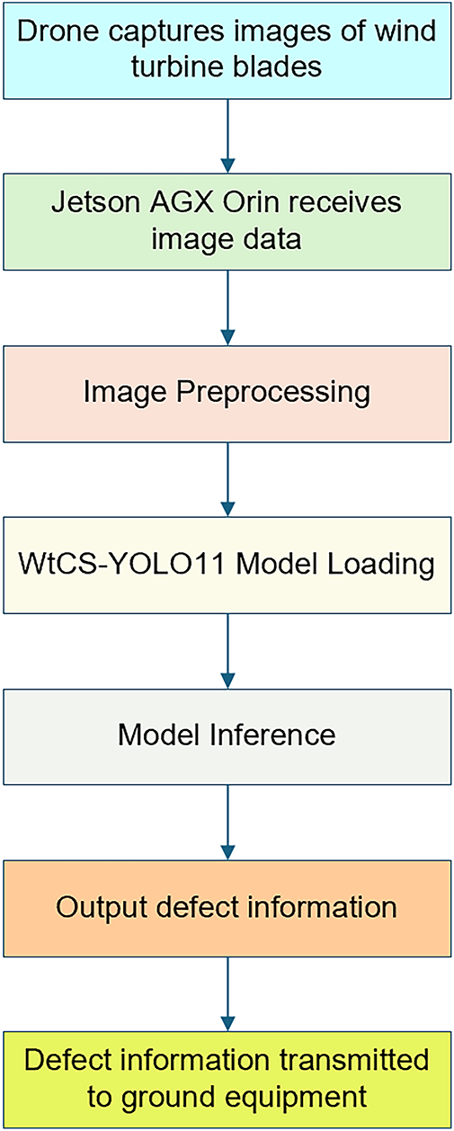
Figure 18: Model deployment execution diagram

4.9 Discussion

This study addresses the limitations of existing wind turbine blade defect detection models, including poor feature extraction, missed small targets, and insufficient bounding-box regression accuracy. It proposes the WtCS-YOLO11 model, which integrates C3k2_WTConv, CBAM, and NWD-Shape-IoU modules, and experimentally validates its effectiveness. C3k2_WTConv expands the receptive field through multiscale wavelet domain convolutions, enhancing detection accuracy while reducing parameters by 52,992 via small convolutional kernels—balancing high precision with lightweight implementation. CBAM’s dual spatial-channel attention mechanism precisely focuses on defect regions while suppressing non-defect areas; heatmaps show its superior background suppression compared to mechanisms such as ECA. NWD-Shape-IoU combines distance metrics with shape adaptability to more accurately quantify the similarity between predicted and ground-truth bounding boxes. Together, these three modules enable the model to achieve an mAP50 of 89.7% and an F1 score of 85.6%, delivering optimal performance. Compared to the baseline YOLO11 model, this model adds only 12,898 parameters while maintaining identical GFLOPs and model size. It achieves 104 fps on NVIDIA Jetson AGX Orin edge devices, far exceeding the 60–90 fps real-time requirements for drone inspections, with storage consumption well below the device’s limits. Comparative experiments demonstrate that it significantly outperforms mainstream models such as YOLO11n and YOLOv9-tiny in mAP50. Furthermore, transferring these improvements to YOLOv8n and RT-DETR-l yields a 0.8% increase in mAP50 for both models, demonstrating the approach’s strong generalization. Compared to the MES-YOLOv8n model proposed in [33], the proposed approach maintains comparable parameter counts while achieving significantly improved detection accuracy, indicating its superior suitability for defect detection in wind turbine blades.

5  Conclusion

The proposed WtCS-YOLO11 model can be directly deployed on inspection drone platforms to realize real-time identification and localization of wind turbine blade defects. This deployment significantly enhances the efficiency and precision of wind farm inspections, providing robust technical support for the health monitoring and operational decision-making of wind power equipment. While this study has achieved phased breakthroughs in model performance and practicality, there remain areas for refinement. For blurred image data generated by drone flight vibrations or high-speed motion, the current sample size is slightly insufficient, failing to fully capture the image quality issues commonly encountered during actual data collection. Additionally, the existing dataset lacks sufficient samples for the paint loss category, leading to suboptimal recognition performance. Therefore, in subsequent work, the dataset must be continuously expanded, with a focus on supplementing blurred image samples related to drone jitter and high-speed motion. This supplementation will enhance the model’s environmental adaptability to complex acquisition conditions. Simultaneously, typical image data for the paint loss category should be purposefully increased, while representative images of paint loss defects should be specifically supplemented. This targeted expansion of the dataset will provide more robust data to optimize the model’s paint loss detection accuracy and reduce false-negative rates. Furthermore, the proposed WtCS-YOLO11 enhancement scheme demonstrates strong generalization, facilitating seamless transfer to other industrial vision inspection scenarios, such as photovoltaic panel crack detection and aircraft engine blade defect identification. This strong generalization capability provides a universal technical reference for the intelligent health monitoring of various industrial equipment.

Acknowledgement: Not applicable.

Funding Statement: This work was supported in part by the Science and Technology Research Project of Henan Province under grants 242102240040 and 222102210087, and in part by the Training Plan for Young Backbone Teachers at Undergraduate Universities in Henan Province under grant 2024GGJS155.

Author Contributions: The authors confirm their contributions to the paper as follows: study conception and design, Yajuan Lu, Yongtao Hu, Jie Li; data collection, Jinping Zhang; analysis and interpretation of results, Yajuan Lu, Jingjing Si; draft manuscript preparation, Yajuan Lu. All authors reviewed the results and approved the final version of the manuscript.

Availability of Data and Materials: The data that support the findings of this study are available from the Corresponding Author, [Yajuan Lu], upon reasonable request.

Ethics Approval: Not applicable.

Conflicts of Interest: The authors declare no conflicts of interest to report regarding the present study.

References

1. Regan T, Beale C, Inalpolat M. Wind turbine blade damage detection using supervised machine learning algorithms. J Vib Acoust. 2017;139(6):061010. doi:10.1115/1.4036951. [Google Scholar] [CrossRef]

2. Du Y, Zhou S, Jing X, Peng Y, Wu H, Kwok N. Damage detection techniques for wind turbine blades: a review. Mech Syst Signal Process. 2020;141:106445. doi:10.1016/j.ymssp.2019.106445. [Google Scholar] [CrossRef]

3. Dimitrova M, Aminzadeh A, Meiabadi MS, Sattarpanah Karganroudi S, Taheri H, Ibrahim H. A survey on non-destructive smart inspection of wind turbine blades based on industry 4.0 strategy. Appl Mech. 2022;3(4):1299–326. doi:10.3390/applmech3040075. [Google Scholar] [CrossRef]

4. Xu D, Wen C, Liu J. Wind turbine blade surface inspection based on deep learning and UAV-taken images. J Renew Sustain Energy. 2019;11(5):053305. doi:10.1063/1.5113532. [Google Scholar] [CrossRef]

5. Juengert A, Grosse CU. Inspection techniques for wind turbine blades using ultrasound and sound waves. In: Proceedings of the 7th International Symposium on Nondestructive Testing in Civil Engineering; 2009 Jun 30–Jul 3; Nantes, France. [Google Scholar]

6. Rizk P, Al Saleh N, Younes R, Ilinca A, Khoder J. Hyperspectral imaging applied for the detection of wind turbine blade damage and icing. Remote Sens Appl Soc Environ. 2020;18:100291. doi:10.1016/j.rsase.2020.100291. [Google Scholar] [CrossRef]

7. Li X, He Y, Wang H, Sun G, Yu J, Du X, et al. Thermal inspection of subsurface defects in wind turbine blade segments under the natural solar condition. IEEE Trans Ind Electron. 2023;71(9):11488–97. doi:10.1109/tie.2023.3335455. [Google Scholar] [CrossRef]

8. Galleguillos C, Zorrilla A, Jimenez A, Diaz L. Thermographic non-destructive inspection of wind turbine blades using unmanned aerial systems. Plastics Rubber Compos. 2015;44(3):98–103. doi:10.1179/1743289815y.0000000003. [Google Scholar] [CrossRef]

9. Li Z, Haigh A, Soutis C, Gibson A, Sloan R. Microwaves sensor for wind turbine blade inspection. Appl Compos Mater. 2017;24:495–512. doi:10.1007/s10443-016-9545-9. [Google Scholar] [CrossRef]

10. Li D, Ho S, Song G, Ren L, Li H. A review of damage detection methods for wind turbine blades. Smart Mater Struct. 2015;24(3):033001. doi:10.1088/0964-1726/24/3/033001. [Google Scholar] [CrossRef]

11. Zhang S, He Y, Gu Y, He Y, Wang H, Wang H, et al. UAV based defect detection and fault diagnosis for static and rotating wind turbine blade: a review. Nondestruct Test Eval. 2025;40(4):1691–729. doi:10.1080/10589759.2024.2395363. [Google Scholar] [CrossRef]

12. Wang L, Zhang Z. Automatic detection of wind turbine blade surface cracks based on UAV-taken images. IEEE Trans Ind Electron. 2017;64(9):7293–303. doi:10.1109/tie.2017.2682037. [Google Scholar] [CrossRef]

13. Yang C, Liu X, Zhou H, Ke Y, See J. Towards accurate image stitching for drone-based wind turbine blade inspection. Renew Energy. 2023;203:267–9. doi:10.1016/j.renene.2022.12.063. [Google Scholar] [CrossRef]

14. Deng L, Guo Y, Chai B. Defect detection on a wind turbine blade based on digital image processing. Processes. 2021;9(8):1452. doi:10.3390/pr9081452. [Google Scholar] [CrossRef]

15. Gao R, Ma Y, Wang T. Early stage damage detection of wind turbine blades based on UAV images and deep learning. J Renew Sustain Energy. 2023;15(4):043305. doi:10.1063/5.0157624. [Google Scholar] [CrossRef]

16. Masita K, Hasan A, Shongwe T. Defect detection on 110 MW AC wind farm turbine generator blades using drone-based laser and RGB images with Res-CNN3 detector. Appl Sci. 2023;13(24):13046. doi:10.3390/app132413046. [Google Scholar] [CrossRef]

17. Ran X, Zhang S, Wang H, Zhang Z. An improved algorithm for wind turbine blade defect detection. IEEE Access. 2022;10:122171–81. doi:10.1109/access.2022.3216613. [Google Scholar] [CrossRef]

18. Gohar I, Halimi A, See J, Yew WK, Yang C. Slice-aided defect detection in ultra-high-resolution wind turbine blade image. Machines. 2023;11(10):953. doi:10.3390/machines11100953. [Google Scholar] [CrossRef]

19. Lv L, Yao Z, Wang E, Ren X, Pang R, Wang H, et al. Efficient and accurate damage detector for wind turbine blade images. IEEE Access. 2022;10:123378–86. doi:10.1109/access.2022.3224446. [Google Scholar] [CrossRef]

20. Jegham N, Koh CY, Abdelatti M, Hendawi A. Evaluating the evolution of YOLO (you only look once) models: a comprehensive benchmark study of yolo11 and its predecessors. arXiv:2411.00201. 2024. [Google Scholar]

21. Rodríguez-Lira DC, Córdova-Esparza DM, Álvarez-Alvarado JM, Romero-González JA, Terven J, Rodríguez-Reséndiz J. Comparative analysis of YOLO models for bean leaf disease detection in natural environments. Agric Eng. 2024;6(4):4585–603. doi:10.3390/agriengineering6040262. [Google Scholar] [CrossRef]

22. Hidayatullah P, Syakrani N, Sholahuddin MR, Gelar T, Tubagus R. YOLOv8 to YOLO11: a comprehensive architecture in-depth comparative review. arXiv:2501.13400. 2025. [Google Scholar]

23. Peng G, Wang K, Ma J, Cui B, Wang D. AGRI-YOLO: a lightweight model for corn weed detection with enhanced YOLO v11n. Agriculture. 2025;15(18):1971. doi:10.3390/agriculture15181971. [Google Scholar] [CrossRef]

24. Wu W, Cheng H, Pan J. Wavelet-enhanced YOLO for intelligent detection of welding defects in X-ray films. Appl Sci. 2025;15(8):4586. doi:10.3390/app15084586. [Google Scholar] [CrossRef]

25. Finder SE, Amoyal R, Treister E, Freifeld O. Wavelet convolutions for large receptive fields. In: Proceedings of the European Conference on Computer Vision—ECCV 2024; 2024 Sep 29–Oct 4; Milan, Italy. Cham, Switzerland: Springer Nature; 2024. p. 363–80. [Google Scholar]

26. Wang W, Tan X, Zhang P, Wang X. A CBAM based multiscale transformer fusion approach for remote sensing image change detection. IEEE J Sel Top Appl Earth Obs Remote Sens. 2022;15:6817–25. doi:10.1109/jstars.2022.3198517. [Google Scholar] [CrossRef]

27. Woo S, Park J, Lee JY, Kweon IS. Cbam: convolutional block attention module. In: Proceedings of the European Conference on Computer Vision (ECCV); 2018 Sep 8–14; Munich, Germany. p. 3–19. [Google Scholar]

28. Fu H, Song G, Wang Y. Improved YOLOv4 marine target detection combined with CBAM. Symmetry. 2021;13(4):623. doi:10.3390/sym13040623. [Google Scholar] [CrossRef]

29. Zhang H, Zhang S. Shape-iou: more accurate metric considering bounding box shape and scale. arXiv:2312.17663. 2023. [Google Scholar]

30. Panaretos M, Zemel Y. Statistical aspects of Wasserstein distances. Annu Rev Stat Its Appl. 2019;6(1):405–31. doi:10.1146/annurev-statistics-030718-104938. [Google Scholar] [CrossRef]

31. Huang J, Wang K, Hou Y, Wang J. LW-YOLO11: a lightweight arbitrary-oriented ship detection method based on improved YOLO11. Sensors. 2024;25(1):65. doi:10.3390/s25010065. [Google Scholar] [PubMed] [CrossRef]

32. Wei J, Ni L, Luo L, Chen M, You M, Sun Y, et al. GFS-YOLO11: a maturity detection model for multi-variety tomato. Agronomy. 2024;14(11):2644. doi:10.3390/agronomy14112644. [Google Scholar] [CrossRef]

33. Ma L, Jiang X, Tang Z, Zhi S, Wang T. Wind turbine blade defect detection algorithm based on lightweight MES-YOLOv8n. IEEE Sens J. 2024;24(17):28409–18. doi:10.1109/jsen.2024.3430351. [Google Scholar] [CrossRef]