Airborne Acoustic Transmission and Terrain Topography at SAINTGITS Amphitheatre: An Analysis of Outdoor Auditory Perception and Comparison of Contour Plots

1  Introduction

Any topographical maps that represent the surface configuration of the earth in multiple dimensions are widely referred and accepted [1]. These maps can distinctly exhibit the three-dimensional contour of a particular region [1,2]. Though the cartographers and experts frequently visit these maps and can interpret the data, the budding learners face barriers [3,4]. The embedded data related to terrain topography and meteorology are vital. The vertical air path in any geographical region is openly influenced by the terrain topography, relative humidity and air circulation [5]. It is inferred that the microclimate has a direct correlation to terrain topography [5]. The propagation of the acoustic wave is dependent on meteorological conditions such as relative humidity, wind speed, atmospheric pressure, temperature and turbulence [6]. At all times in a homogeneous atmosphere, the near-ground transmission characteristics of low-frequency acoustics are primarily governed by the surface boundary conditions [7]. A few other factors related to outdoor sound propagation are geometric dispersion, absorption by the molecules in the atmosphere, reflection, refraction, diffraction and scattering [8]. In the most recent literature, it has been reiterated that the transmission of sound in urban locales is highly dependent on the meteorological conditions, that in turn causes refraction and scattering of acoustic output [9]. Therefore, the monitored levels of acoustic pressure will certainly manifest a diurnal transient behaviour. Since the monitoring and recording procedures of Sound Pressure Level (SPL) are well-defined and economically viable, it is the commonly used attribute to emulate the intensity of acoustic transmission [10]. Interestingly, the perfect taming and control of sound sources can be greatly achieved by predictive analyses of outdoor acoustic propagation [11].

In ancient days, during the Roman regime, people gathered at the open-air theatres (amphitheatres) for entertainment, performance and sports [12]. The Flavian Amphitheatre in Rome (Colosseum) was the most famous and influential amphitheatres of ancient days [13–15]. The ancient acousticians had carefully designed the open-air theatres to impart and ascertain the uniqueness at all stages such that even the entire audience in the last rows could encapsulate the complete essence of the performance [16–19].

A modest and appreciable research effort was nurtured and taken care of at SAINTGITS, an Autonomous Engineering institution in South India (Fig. 1). Unlike the environmental noise pollution in urban regions, since SAINTGITS is at a rural locale, the effect of traffic noise interference has been completely neglected [20,21].

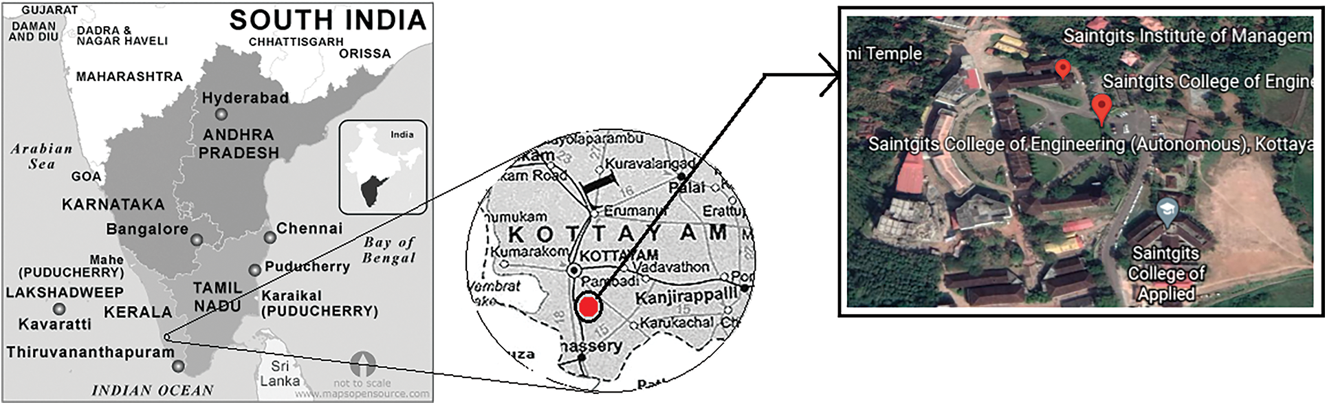
Figure 1: Satellite imagery of SAINTGITS campus, Kottayam District, Kerala State at down South-West of Indian Subcontinent

The lush and green campus encompasses the iconic amphitheatre, SAINTGITS AMPHI. An exclusive and novel study was conducted to analyse the airborne acoustic transmission pattern at SAINTGITS AMPHI and to correlate it with its naturally carved terrain (Fig. 2). The campus encourages sustainable research initiatives that address one of the seventeen Sustainable Development Goals (SDG) of the United Nations, the SDG 11: Sustainable Cities and Communities. A few of the research activities at SAINTGITS include the energy analyses of in-house built structures, quantification of the environmental benefits of Green Facades and the atmospheric cleansing capability of Green retrofits [22–25].

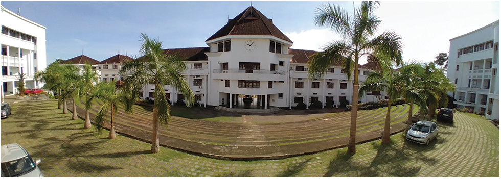
Figure 2: Panoramic imagery of SAINTGITS AMPHI–The Arc-shaped twelve stair iconic Amphitheatre: View from the first floor of Centre Lecture Complex (CLC)

2  Methodology

The recreational facilities at the scenic campus of SAINTGITS are plenty, both for the mind and body of every individual associated with the campus (Fig. 3). It includes the curricular, co-curricular and leisure hours which are evenly spread across the entire calendar days. All the major stakeholders, the student community in particular, indulge themselves in all activities that take place on campus.

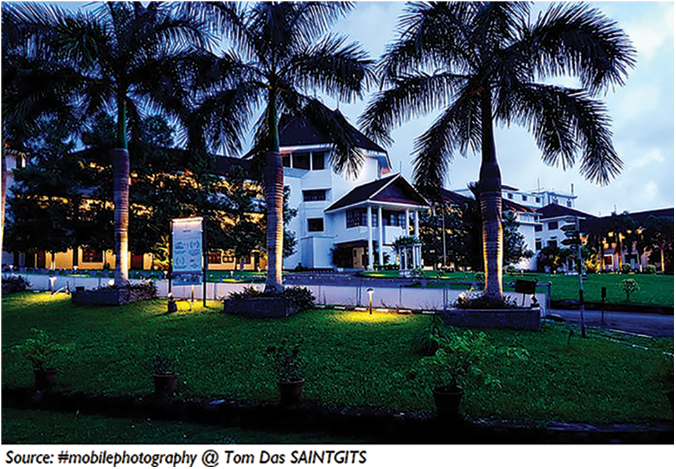
Figure 3: The post-monsoon scenic view of near to dusk SAINTGITS campus

The amphitheatre at SAINTGITS, one of the common places for recreation, is centrally located between the Centre Lecture Complex (CLC) and the Administrative Block (AB). It has a modest gradient from CLC to AB, evenly distributed at 12 levels to comfortably accommodate the gathering. Therefore, the acoustic design of audience seating at amphitheaters includes an inherent altitude gradient between the front-most and rear most seating, scientifically christened as the mechanism of the seat-dip attenuation [26]. Throughout the arc at each level, the plateaued surface has a radial seating width of 1½ metre and, a quarter of a meter as the height difference between the adjacent levels (Fig. 4). Hence, the audience can receive the complete performance in their comfort. A recent case study has addressed the extent of occupant comfort at SAINTGITS AMPHI [27].

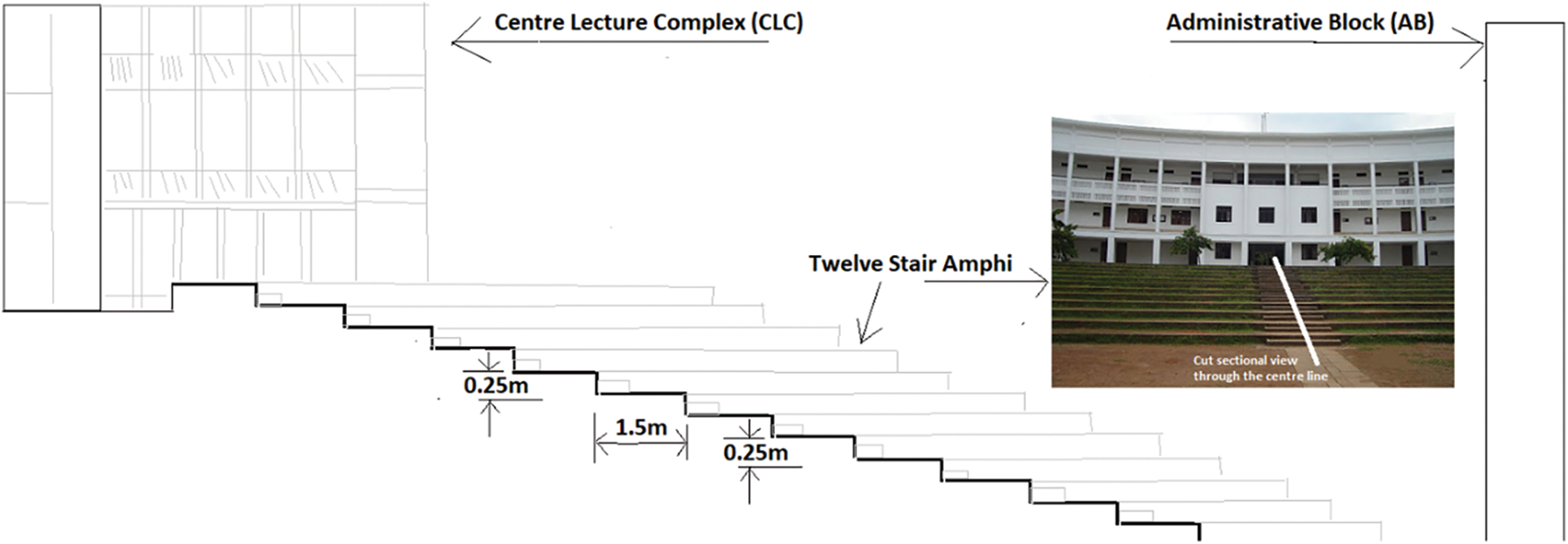
Figure 4: Twelve stair naturally carved Amphitheatre at SAINTGITS–The cross-sectional view through the centre of the Amphitheatre illustrates the location of CLC and AB, with reference to the SAINTGITS AMPHI

This paper expounds and analyses the airborne acoustic transmission over the entire SAINTGITS amphitheatre with the aid of the auditory module of the simulation freeware, the EASE Focus-3, conceived and rolled out during the year 1999. The final phase elaborates the terrain topology over the locale.

EASE Focus-3 is the third version of the acoustic simulator which integrates the acoustic simulation program for 3D modelling of line arrays, sub arrays, digitally steered columns and conventional loudspeakers [28]. More than five dozen loudspeaker manufacturers had immensely contributed to developing the direct sound simulation of complex sound systems in EASE Focus-3. BOSS Professional, Yamaha, Shure, Tannoy and Martin Audio are a few of the renowned acoustic signatures available in the standard library of EASE Focus-3. The broad scope and features of this freeware include the simulation of auditory waves from different sound sources, acoustic analyses of widespread multiple audience areas, flexibility in receiver location with curved and inclined seating, depth of sound coverage, frequency response and computation of tailored Finite Impulse Response (FIR) for each venue. In short, EASE Focus-3 helps the system designers to determine the optimal setup for a given venue [28].

In this work, the modelled acoustical layout at the entire SAINTGITS AMPHI consists of 12 stair seating for the audience, the performance stage and the backstage. The initial analysis and simulation (termed as Base case from hereafter) assume the airborne acoustic transmission to occur in three regions namely (a) the audience module as rectangular with dimensions of 100 m (width) × 80 m (depth), (b) the main stage as a regular trapezoid (25 m front width, 80 m back width and 15 m depth) and (c) the backstage as a perfect square of size 80 m (Fig. 5). The Main stage and Audience module are 15 m apart. Collectively, the three modules of the Base case occupy a 15,188 m2 area and are assumed to be at the same level.

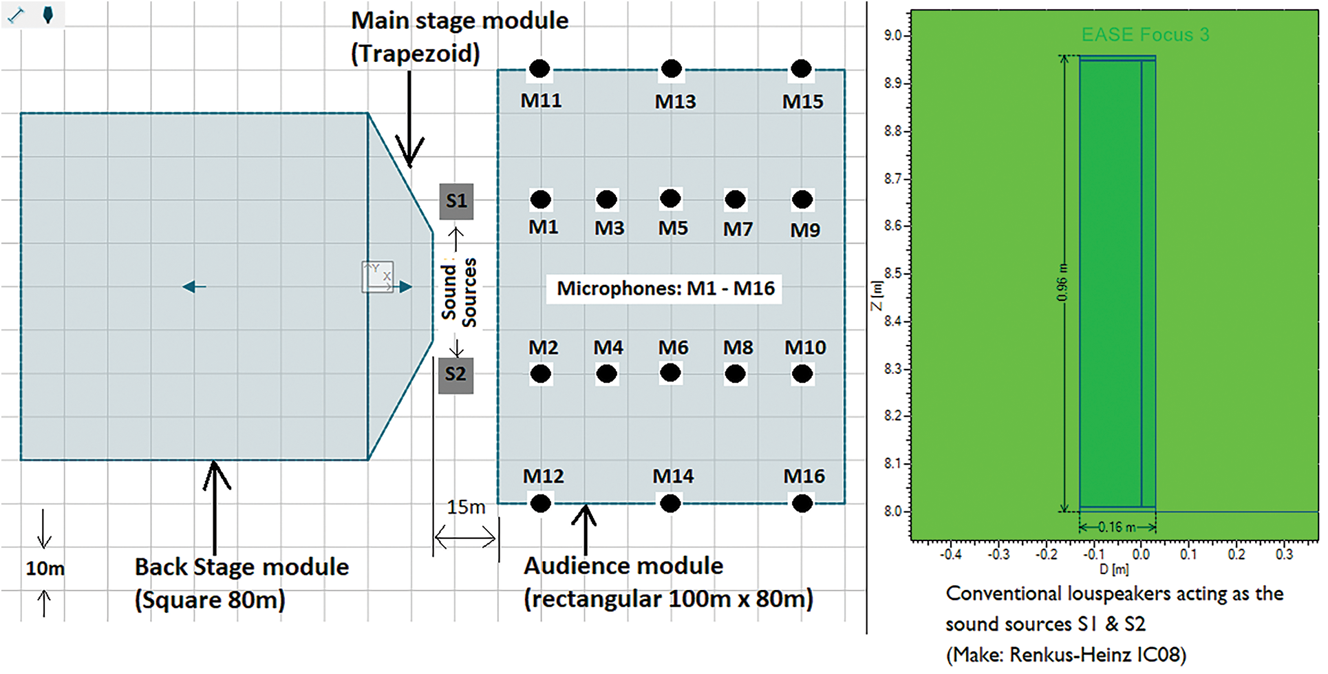
Figure 5: Base case model: Three designated regions with the two positioned sound sources and sixteen microphones to model the airborne acoustic transmission at SAINTGITS AMPHI–(a) Audience, (b) Main stage & (c) Backstage modules

Whilst the two sound sources (make: Renkus-Heinz IC08) were positioned horizontally 40 m apart to achieve wide auditory transmission, sixteen microphones were aligned at various altitudes to collectively emulate the presence and perception of the audience (Fig. 6).

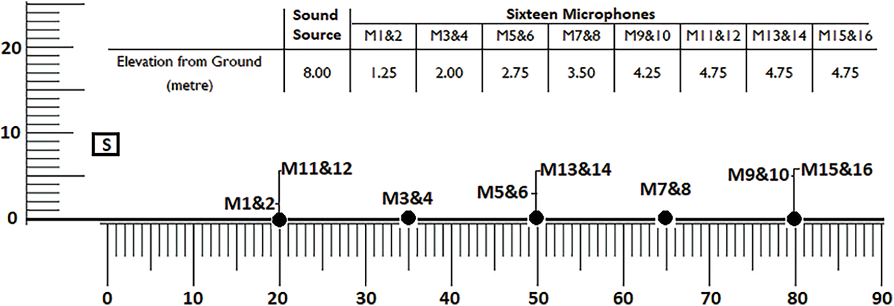
Figure 6: Distance Chart indicating the horizontal spacing and elevation of Sound Sources (S) and Microphones (M) at the Base case model of SAINTGITS AMPHI

In the Advanced case model, the terrain-centric variations were accommodated. The twelve stair amphitheatre was modelled, taking into account the level difference of each stair. Furthermore, sector-wise divisions were performed to analyse the in-depth perception of the auditory level. Three main sectors (Sector angle = 60°) were demarcated (Sectors A, B & C) and each main sector contained six exclusive sub-sectors (Fig. 7). To recommend a safer configuration for richer auditory perception in the Audience module of the Advanced case model, the analyses were extended by substituting the conventional speakers with BOSS professional array systems.

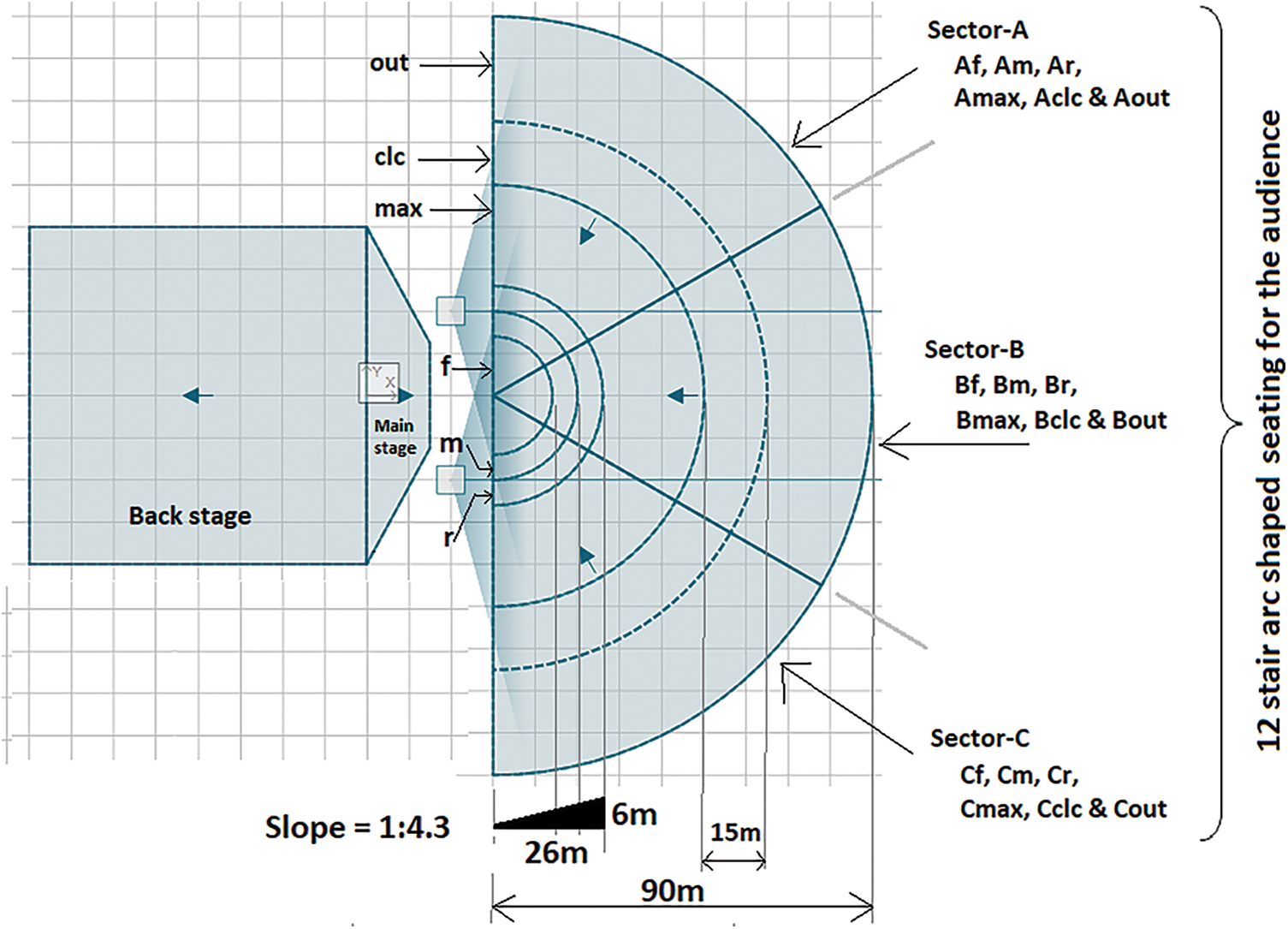
Figure 7: Advanced case model: The realistic preparatory model with three main sectors and six sub-sectors to simulate the auditory perception at SAINTGITS AMPHI

Though the sector-wise segregation improvises the ease of analyses, more footfalls were witnessed in the main sector B. To be more specific and to remain realistic, at the entire twelve stair amphitheatre, the enthusiastic live audience always occupied the initial three sub-sectors in the main sector B (Bf. Bm & Br, respectively). The arc-shaped three-storied built structure (Centre Lecture Complex) occupied the ‘clc’ sub-sector (clc) in the entire main sector B and half of the adjacent regions in both the main sectors A & C. Hence, the sub-sectors Aclc, Bclc and Cclc are structural hindrances to the outreach of live performances beyond Amax, Bmax and Cmax.

An overview of the sub-sector categorized sector-wise, and the gradient details are indicated in Table 1. The sub-sectors Aout, Bout and Cout are the farthest among all the sub-sectors. Maximum occupancy happens in the foremost three sub-sectors, spread across all the main sectors. Throughout the first three subsectors of the audience module, the model gradient was calculated as 14.3 , which is at par with the realistic slope at SAINTGITS AMPHI.

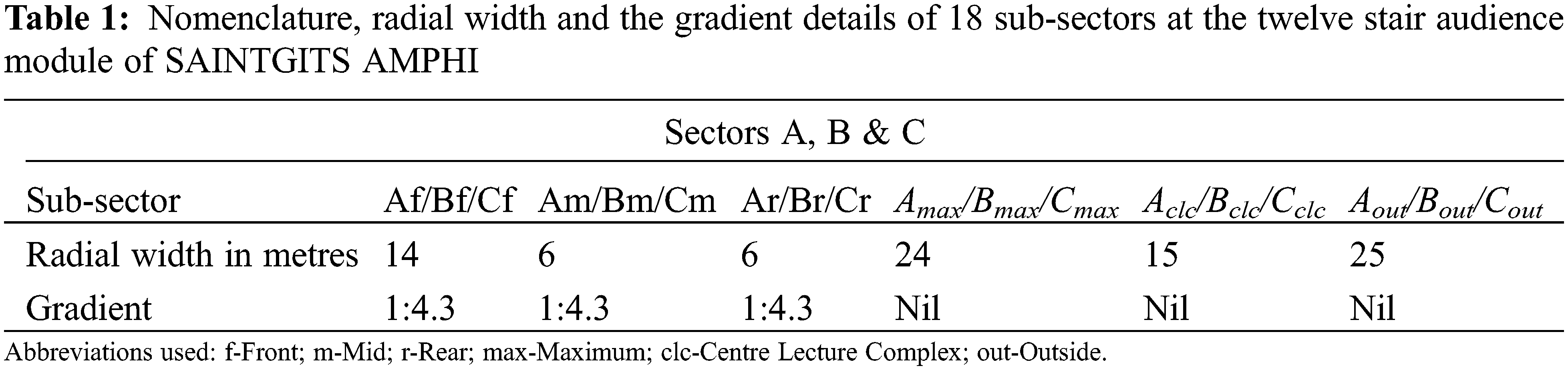
Though the tabulations in Table 1 explicitly specify the radial spacing and respective surface gradient at individual main sectors and sub-sectors, a vivid image of the elevation contours of the terrain is essential. Since the acoustic propagation over non-flat terrains is complex, several researchers have analysed it through comparative studies and models [29].

The culmination of this work includes the topography analyses of SAINTGITS campus, in particular, the terrain topography of SAINTGITS AMPHI. A broader perception of the entire campus and its surroundings were generated, both as axonometric view and topology plots from CADMAPPER, an instant CAD file generator for any location on earth (Fig. 8). The former view helps to identify the relative location of built structures within an area under consideration. Since it is freeware, by default, the coverage area for free analysis is restricted to 1 km2. In general, the axonometric view serves as the base to analyse the natural air flush over certain terrain. While the plot that accommodates 112 buildings and spans a total area of 0.816 m2 was developed in CADMAPPER, the overall height of all built structures was assumed uniformly as 10 m (Fig. 8).

Figure 8: CADMAPPER imagery of SAINTGITS campus: Axonometric view of the built structures at neighbouring locales (height 10 m assumed throughout) and elevation contours of the terrain encompassing the campus for a 0.816 m2 area

The satellite imagery over the campus was accessed from Google Earth Pro (GEP). The terrains over SAINTGITS AMPHI were traced, both in the longitudinal and transverse direction, using GEP’s ‘Add Path’ feature. The trace covered the entire twelve stair amphitheatre. The embedded terrain data points were retrieved and displayed with QuikGrid, a freeware to represent the terrain, either as two or three-dimensional contours. Further, the results were analysed to reiterate the reliability of the obtained terrain gradient plots.

3  Results and Discussion

This novel study at SAINTGITS was done to exhibit the immense simulation potential and versatility of the two freeware, EASE Focus and QUIKGRID. The airborne acoustic transmission and terrain topography were analysed in detail. For a detailed discussion, the results are categorized into five subsections: (3.1) influence of vertical beam angle on SPL(A) & SPL(Z) in the Base case model, (3.2) SPL vs. distance: juxtaposing the SPL(A) with SPL(Z) in Base case model, (3.3) frequency response of the receiving ends (microphones) in Base case model, (3.4) acoustic transmission over SAINTGITS AMPHI in Advanced case model and (3.5) terrain-dependent acoustic transmission over SAINTGITS AMPHI.

3.1 Influence of Vertical Beam Angle on SPL(A) & SPL(Z) in Base Case Model

In the Audience module of the Base Case model, two Renkus-Heinz (IC-08) sound sources were chosen to provide the required auditory perception. The perception of loudness by the human ear was scientifically emulated with the help of orderly arranged microphones (Figs. 5 and 6). The beam angle of the sound source, which determined the area covered by its acoustic transmission was initially set at zero degrees. The distributed levels of sound pressure and the respective distribution percentages (at zero-degree beam angle) across the entire amphitheatre (Audience Module) were analysed individually for SPL(A-Weighting) and SPL(Z-Weighting) (Fig. 9).

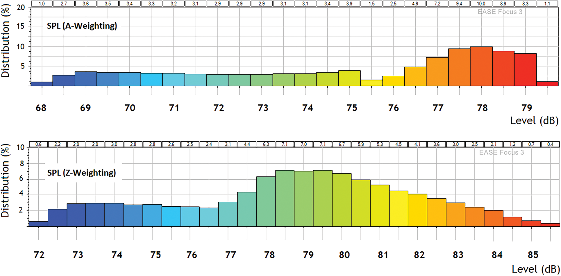
Figure 9: Base case analyses of maximum and minimum SPL distribution across SAINTGITS AMPHI (Audience Module) for SPL(A) and SPL(Z) at zero beam angle

By analysing the SPL(A-Weighting) at a zero-degree beam angle, the recorded value of average SPL(A) was 74.9 dB. Though the entire range of SPL(A) was between 68 and 79.5 dB, the maximum (78 dB) and minimum (68 dB) were recorded respectively for 10% and 1% of the total SPL(A) distributions. The SPL(Z-Weighting) or ZERO frequency-weight was first introduced in the year 2003 as the International Standard IEC 61672: 2003. It is currently christened as IEC 61672-2 and is followed worldwide [30]. At zero-degree beam angle, the average SPL(Z) was recorded as 78.8 dB.

Whilst the physical hearing capability of a human being is represented by the A-Weighting curve, the Z-Weighting mainly focuses to analyse the sound source. The former is commonly used as an instant scientific measure of loudness. It also has the flexibility to interpret itself as sound power or sound pressure levels [31]. Since sustainable nurturing and the well-being of humans are of great concern, it is advisable to adhere to the safest sound pressure level that can be perceived for longer durations. In short, the SPL(A) is audience-centric and SPL(Z) is source centric.

Furthermore, at the Audience module of the Base case model, a wide range of beam angles (varying from −4.0° to +4.0°) for sound source S1 (see Fig. 5) were projected to get an insight into the respective maximum and minimum values of SPL(A) & SPL(Z), alongside the average values and distribution percentages (Table 2).

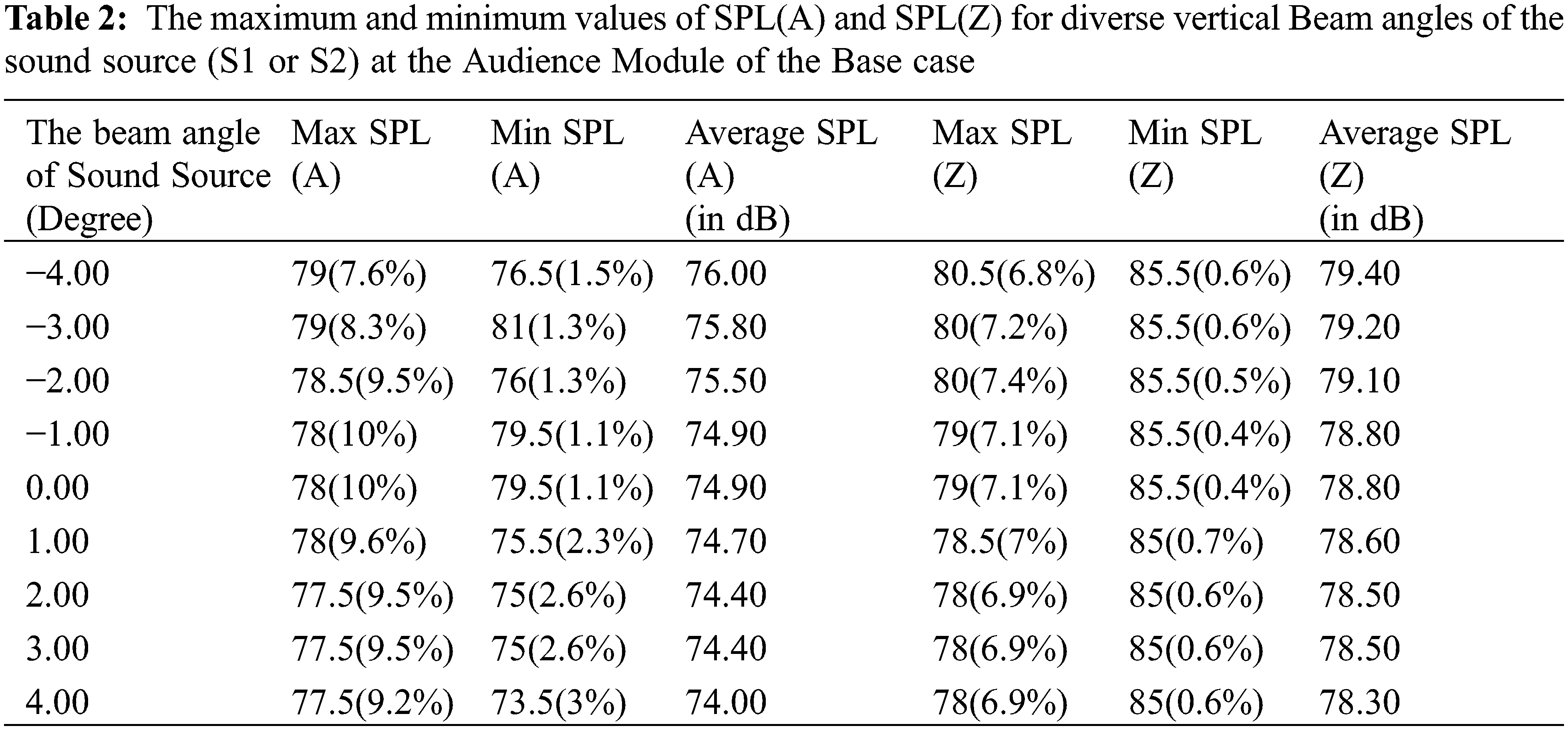
U.S. Occupational Safety and Health Administration (OSHA) has reported the comfortable and safest level of sound pressure that any human ear can perceive for longer durations as less than or equal to 85 dB [32,33]. Another study on the interiors of a fully functional woodworking factory has carried out the acoustic measurements as A-weighting [34]. Hence, an analyses of SPL(A) is more relevant than SPL(Z). The average value of SPL(Z) is approximately 3.8 dB higher than SPL(A). As the beam angle is varied from −4.0° to +4.0°, the difference in the average values of SPL(A) and SPL(Z) changes from 3.4 to 4.3 dB, exhibiting a linearly increasing trend. In particular, among the analysed range of beam angles, a source beam angle of −4.0° will certainly disperse the entire sound pressure to the audience (Fig. 10).

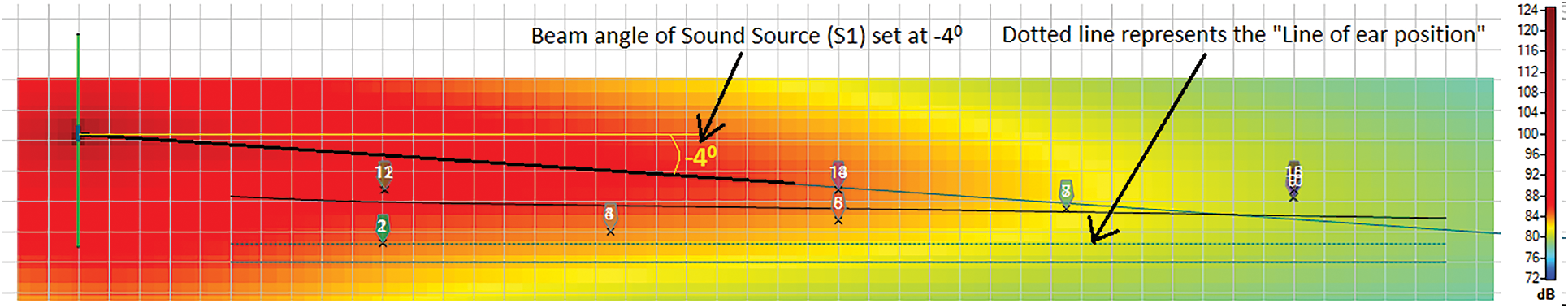
Figure 10: Effective dispersion of sound pressure at safer levels with −4.0° beam angle

If the beam is inclined more to the other direction (positive side), the sound dispersion too happens upwards. Therefore, to experience the richness of auditory performance (at safer upper limits of 85 dB throughout the line of ear position) with the current configuration at the Audience module of the Base case model (see Fig. 5), a beam angle of −4.0° is highly recommended for both sound sources S1 and S2 (Fig. 10).

After analysing the effects of vertical beam angle on sound dispersion, the succeeding session explores the influence of distance on the behavioural pattern of both SPL(A) and SPL(Z).

3.2 SPL vs. Distance: Juxtaposing the SPL(A) with SPL(Z) in Base Case Model

The Audience module of the Base case model has an auditory depth (usually the distance from the sound source to the audience at the farthest point) of 80 m. Hence, in the most ideal case, the audience is believed to be stationed at random locations inside a total area of 80,000 m2 (Fig. 5). The values of sound pressure level are dependent on the distance from the sound source. If the SPL value at a pre-determined point (reference values and points) is available, the corresponding values of SPL at any known distance away from the reference location can be analytically determined, see Eq. (1).

L2=L1−|20logr1r2| (1)

where,

r1 = Reference point

r2 = Any known point away from r1

L1 = Reference Sound level at r1

A well-focused comparison of the values of SPL(A) and SPL(Z), analysed individually for a range of beam angles (−4.0° to +4.0°), are plotted against the linear depth (0–80 m, an indicator for expected occupancy at amphitheatre) of the Audience module of Base case model (Fig. 11).

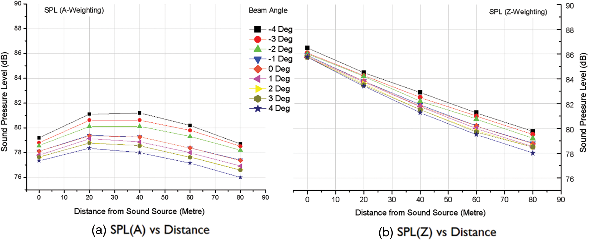
Figure 11: A stark comparison of SPL(A) and SPL(Z) against the linear distance from the sound source for beam angles ranging from −4.0° to +4.0°

The plotted values of SPL(A) confirm the adherence of the auditory level to the safer threshold of 85 dB, irrespective of the beam angle. At certain negative ranges of beam angles (−4.0°, −3.0° and −2.0°), the SPL(A) at halfway from the sound source (40 m) hovered at the same level as the values at a quarter distance (20 m). While the distance varied from 20 to 40 m, the decaying of SPL(A) for beam angles ranging from −4.0° to 0.0° was negligible (<0.15° dB). However, the rate of decay was prominent from 40 m until the farthest point (80 m).

A source-centric analyses of the sound pressure level (Z-Weighting) exhibits a steep decline, right from the source point until the farthest end of the Audience module in the Base case model. At every 20 m after quarter distance from the sound source, for all the modelled beam angles, the average decay was 1.67 dB. An overall view of the drop in sound pressure level had displayed the least drop as 1.68 dB at −4.0° beam angle. The maximum decay was recorded as approximately 2 dB (4.0° beam angle).

To comprehend, irrespective of weighting procedures, the range of SPL concerning the beam angles and the linear distance from the sound source, a beam angle of −4.0° will render richer acoustic transmission throughout the length and breadth of the Audience module in the Base case model.

As the last parameter to analyse in the Base case model, the frequency responses of ten centrally arranged microphones are comprehended in the following session.

3.3 Frequency Response of the Receiving Ends (Microphones) in Base Case Model

The frequency response of any receiving device (mainly microphones) symbolizes its sensitivity to varying levels of frequencies [35]. It can emulate the entire audible sound range of 20 Hz to 20 kHz. Ten linearly arranged microphones were modelled inside the Audience module of the Base case and their responses to an octave band of frequencies ranging from 31.5 Hz to 16 kHz were obtained on a logarithmic scale (Fig. 12).

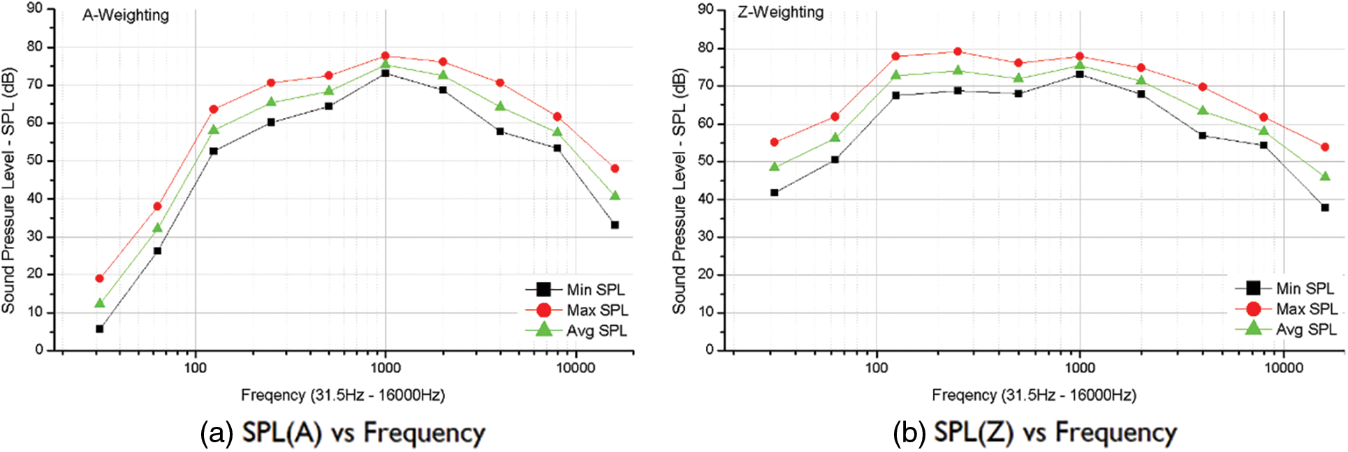
Figure 12: A logarithmic plot of the overall frequency responses of ten microphones, arranged linearly at the Audience module of the Base case model: plots obtained for an octave band of frequencies ranging from 31.5 Hz to 16 kHz

Both A and Z weightings recorded their respective maximum sound pressure levels at octave frequencies of 1000 and 250 Hz. However, SPL(Z) had two more frequencies (125 and 250 Hz) which were nearer to its maximum SPL. Though the average SPL for A-weighting and Z-weighting experienced similar trends throughout, the variations were more significant for frequencies 31, 5, 63 and 125 Hz. At all octave frequencies from 1 to 8 kHz, there were subtle differences in the respective values of sound pressure levels. To be more specific, at exact 1000 Hz, the difference in average values of SPL(A) and SPL(Z) was merely 0.05 dB. Interestingly, even the maximum values of the SPL(A) and SPL(Z) were well inside the safer and sustainable auditory level of human ears.

In a nutshell, irrespective of the weightings (SPL(A) and SPL(Z)), the general trend of frequency responses of the receiving instruments in the Audience module of the Base case model were almost similar.

Having discussed enough the basic parameters in the base case model, now the discussion proceeds to consider the realistic acoustic space as the Advanced case model.

3.4 Acoustic Transmission over SAINTGITS AMPHI in Advanced Case Model

A realistic analysis and discussion on the airborne acoustic transmission over the amphitheatre at SAINTGITS can be elucidated by modelling the entire recreational locale as the Advanced case model. Whilst the Base case model assumed the Audience module as a single entity rectangular region, the Advanced case replicated the geometrical form of the twelve stairs SAINTGITS AMPHI as major sectors and sub-sectors (Fig. 7 and Table 1).

Since SPL(A) predominantly takes care of the auditory perception by any human ear (audience-centric), the prime focus in the Advanced case model was to follow with the A-Weighting, rather than the source-centric SPL(Z).

The arc segment “clc” falls within the entire sector B ( Bclc) and equally to a quarter of the adjacent sectors ( Aclc and Cclc ) accommodates the three-storied Centre Lecture Complex (CLC). Hence, any acoustic transmissions from the sound sources S1 & S2 are intermittently obstructed by CLC’s vertical façade. The euphoric audience, gathered randomly within the arc segment “out” contained in all the sectors ( Aout , Bout & Cout ) is therefore out of direct sight for any on-stage performer and vice-versa. In short, the resultant airborne acoustic transmission from S1 & S2 can maintain its entire sheen and quality, only until the outermost circumference of the arc segment “max” in all the sectors ( Amax , Bmax & Cmax ) (Fig. 13).

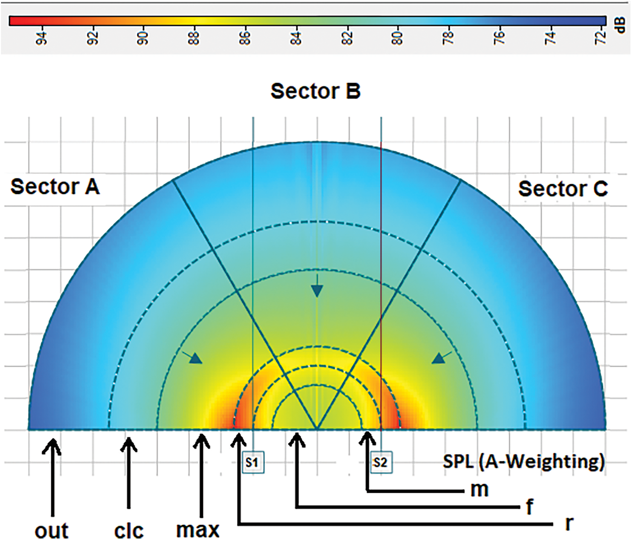
Figure 13: Visualizing the dispersion of Sound Pressure Level at the Audience module of SAINTGITS AMPHI: Advanced case model

Twelve stairs of the naturally carved amphitheatre (SAINTGITS AMPHI) are lodged within the complete arc segments “r” & “m” ( Ar , Br , Cr , Am , Bm & Cm ). The audience are presumed to be at these locations (Fig. 12). Unfortunately, at −4.0° beam angle, the range of SPLs (85.4 dB Min to 93.8 Max) at these sub-sectors are above the widely researched and accepted sustainable safer auditory threshold of any human ear (85 dB). However, the upper limits of SPLs at the sub-sectors Bm and Br modestly hovered at 88.1 dB. Incidentally, during the major annual techno-cultural activity (NAKSHATRA), the majority of the audience at SAINTGITS AMPHI gathers well inside the sub-sectors Bm , Br and Bmax to capture the unobstructed view of the main stage.

In-depth scrutiny of the overall values of SPL, collectively for these three sub-sectors found that at a vertical beam angle of −4.0°, the range of SPL(A) was within the band of 81.9 to 88.1 dB (Fig. 14).

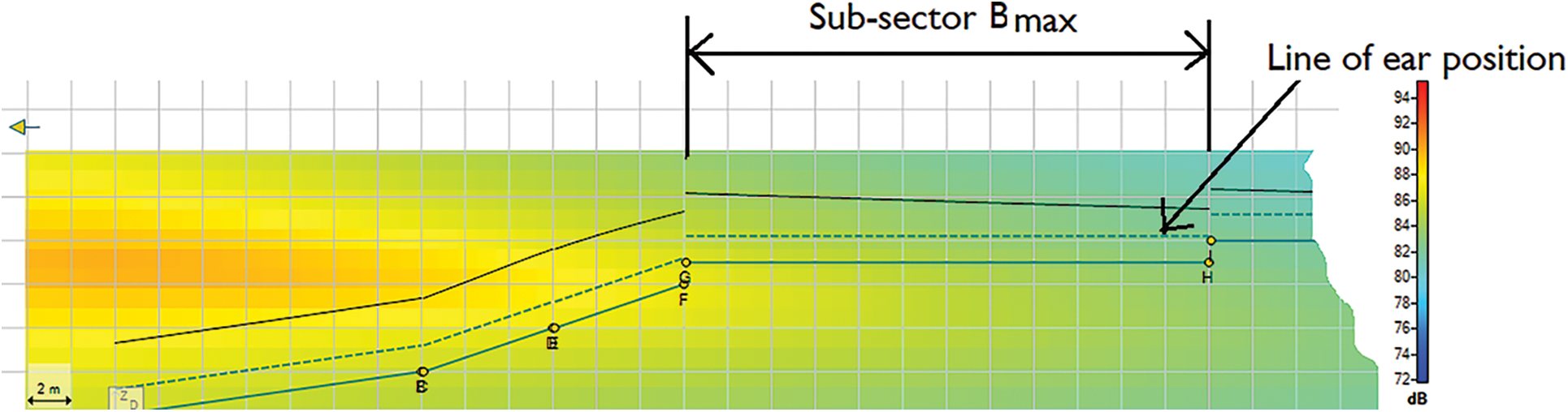
Figure 14: The safer auditory threshold attained at the sub-sector Bmax with a projected vertical beam angle of −4.0°. Ear height is assumed to be at the sitting position

Furthermore, the sub-sector Bmax is approximately double the area of both Br and Bm and the recorded range of SPLs (beam angle at −4.0°) were between 81.9 to 85.6 dB (Fig. 12a). Hence, during live acoustic performances on the main stage, to maintain a safer auditory level, it is advisable to encourage the occupancy in sub-sector Bmax at the Audience module than at any other sub-sectors.

The analyses were extended to the immediately advanced phase by substituting the Renkus-Heinz loudspeakers with a BOSS professional 4-array system (Fig. 15). For any of the annual cultural festivals taking place at SAINTGITS, the array-type speaker systems are preferred over conventional columns. Lower attenuation of sound pressure over distance, spherical propagation path and both horizontal and vertical spreading of sound waves are a few of the key advantages of professional array systems over the column types [36]. It is quite unfortunate to observe that in several instances, the SPLs are much higher than the safer hearing threshold (85 dB).

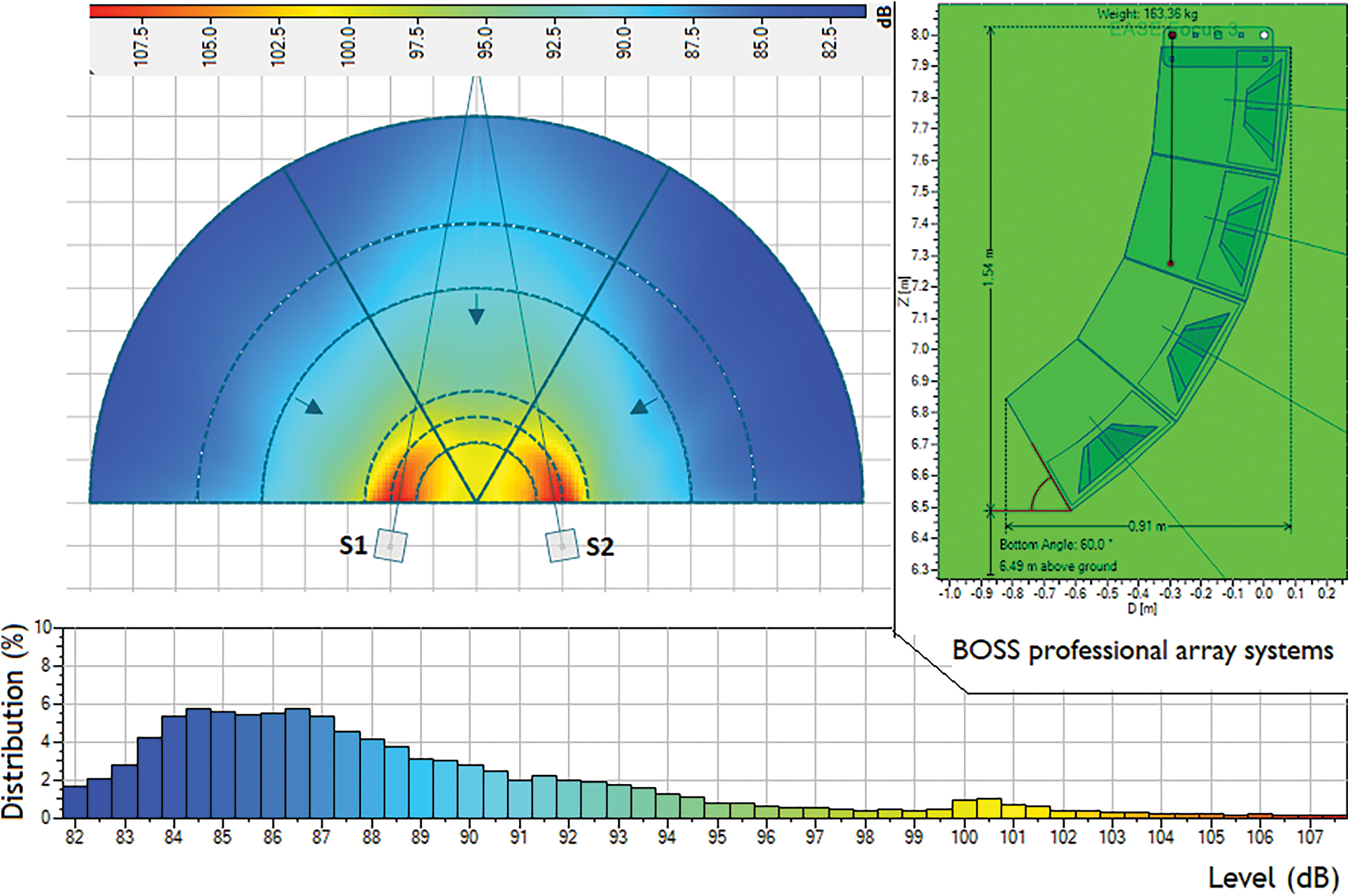
Figure 15: Distribution of SPL(A) at the Audience module of the Advanced case model: Boss professional 4-array loudspeaker systems are used as the sound sources

The same scenario had been recreated with two array type loudspeakers (S1 & S2), arranged 10 m away from the audience module and stationed 40 m apart. The horizontal beam angles are set at −10.0° and +10.0°, respectively for S1 & S2 (Fig. 15). Each of the four arrays is arranged at unique vertical beam angles (5°, 10°, 15° & 20°).

Whilst 27.7% of the total distributions had their SPLs within the safer hearing threshold (82–85 dB), more than 5.5% of SPLs were equal to or more than 100 dB (100 to 107 dB). The average SPL was almost 89 dB. The safer limits could be observed only at the most unoccupied sub-sectors Aout , Bout & Cout . Conversely, in the largely occupied regions in front of the main stage, the range of SPLs (95.7 to 107 dB) were too alarming (Fig. 15). It is an extremely unhealthy practice that demands urgent rectification.

A modified configuration for the Audience module was suggested to address the issues concerning the perpetuation of sustainable auditory levels. The two 4-array loudspeaker systems (S1 & S2) were set 40 m away from the Audience module, 80 m apart and maintained the horizontal beam angle of −10.0° and +10.0°, respectively for S1 & S2 (Fig. 16).

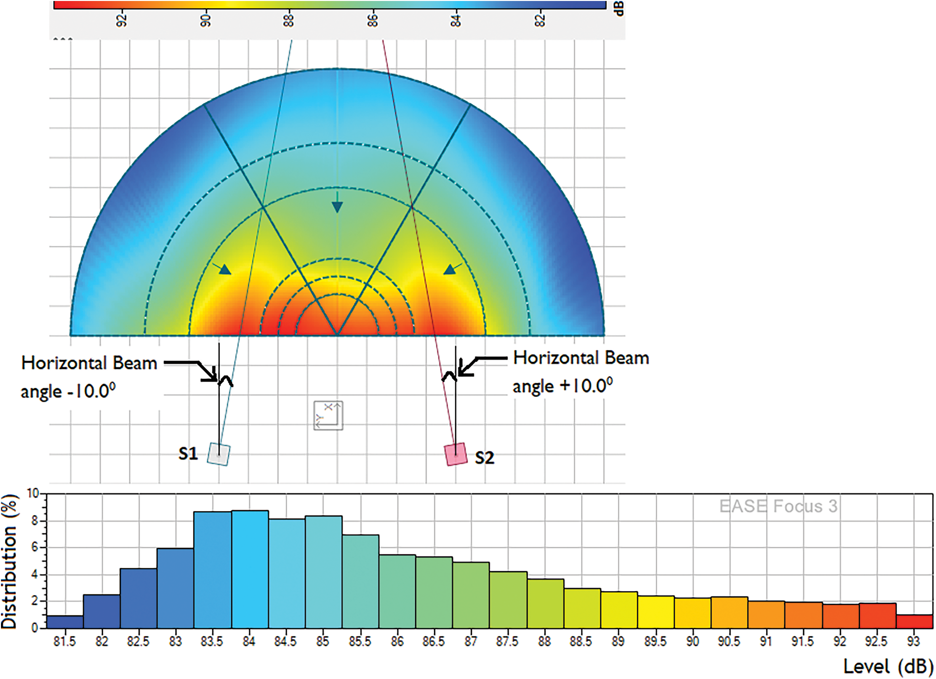
Figure 16: A modified configuration of the 4-array system to attain sustainable auditory levels and the corresponding SPL(A) distribution

The acoustic analyses revealed that nearly 48% of the total SPL distributions (81.5 and 93 dB) hovered below the safer auditory level (85 dB) and the average SPL(A) was approximately 86 dB (Fig. 16). Hence, the modified configuration had been identified to be safer for longer durations.

Since the outdoor acoustic transmission is highly influenced by the physical structure at the boundary layers, a quantifiable overall discussion on the same follows in the immediate session.

3.5 Terrain-Dependent Acoustic Transmission over SAINTGITS AMPHI

The propagation of outdoor sound is dependent on two broad factors: (i) attenuation due to the influence of the earth’s surface and (ii) the atmospheric absorption of the sound [37,38]. The sub-components of the above factors include the atmospheric absorption due to air molecules, physical barriers, levels of vegetation, ground absorption, wind speed, temperature, presence of water bodies and terrain gradient [9,39,40]. To be precise, if the airborne sound propagation is over water bodies, the acoustic waves travel according to their respective frequencies [40].

The application of acoustics is being practiced and further explored to analyse the stability of rivers and hydraulic structures: monitoring the sediment transport processes in rivers is one of the applications [41]. Similarly, if the airborne sound propagation is closer to the ground, the porosity of the ground surface, its related acoustical properties and finally, the meteorological conditions of the locale influence the acoustic transmission [39,40,41].

Higher levels of sound pressure are attributes of increased mean wind speeds. Interestingly, the distance between the sound source and the audience zone also affects the SPLs. The wind effect is prominent for larger distances [9]. Since wind speed is one of the major governing factors that affect the outdoor acoustic transmission, a wind rose was plotted with the renowned freeware, WRPLOT (version 8.0.2), powered by Lakes Environmental Software (Fig. 17)

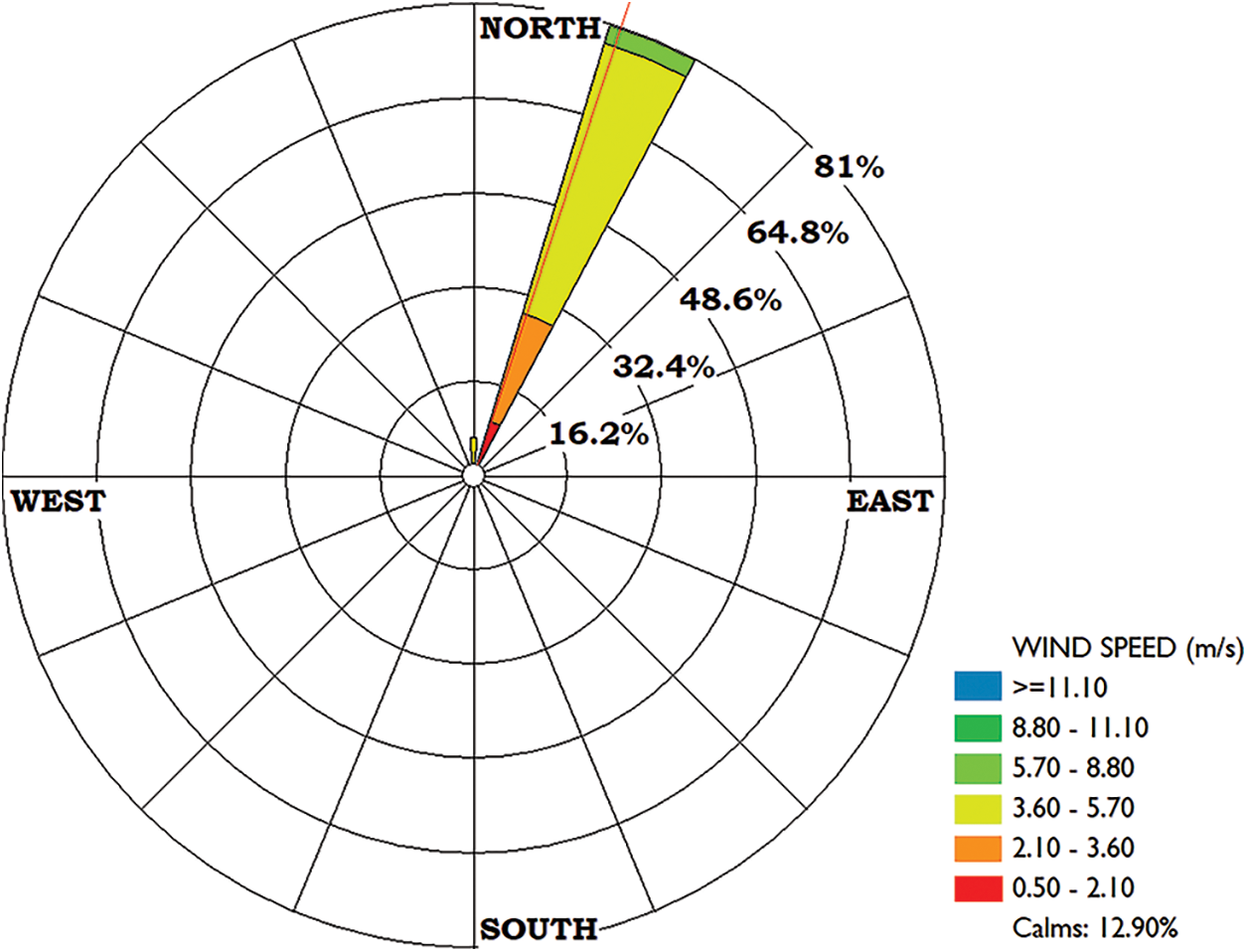
Figure 17: The wind rose plotted for the month of January 2021 at Kottayam District, Kerala State, India

The meteorological data for the month of January 2021 was retrieved from the archives of https://timeanddate.com. The data about the wind speed and wind direction were plotted with WRPLOT. A detailed analysis revealed that the noticeable wind speed was in the wind class 3.6 to 5.7 m/s. It accounted for nearly 55% of the total distribution and was prominent in the North-South direction. Whilst the least recorded average wind speed was 1.3 m/s, the entire region was calm for a considerable period (Fig. 17).

The satellite imagery of SAINTGITS, in particular, the imagery above SAINTGITS AMPHI was accessed from Google Earth Pro (GEP) and the two dimensional and three-dimensional plots of the contour were generated and analysed (Figs. 18 and 19). The data points were positioned in two main patterns, the longitudinal (Fig. 18) and the transverse (Fig. 19) pattern. Whilst the former pattern accommodated 663 data points by progressing 1180 m in the longitudinal direction, the latter generated the plot with mere 159 data points during its 690 m transverse progress.

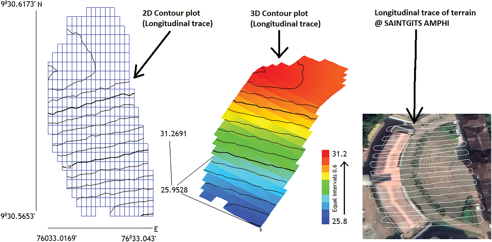
Figure 18: The terrain topology of SAINTGITS AMPHI, measured in the longitudinal direction, represented as 2D and 3D contour plots

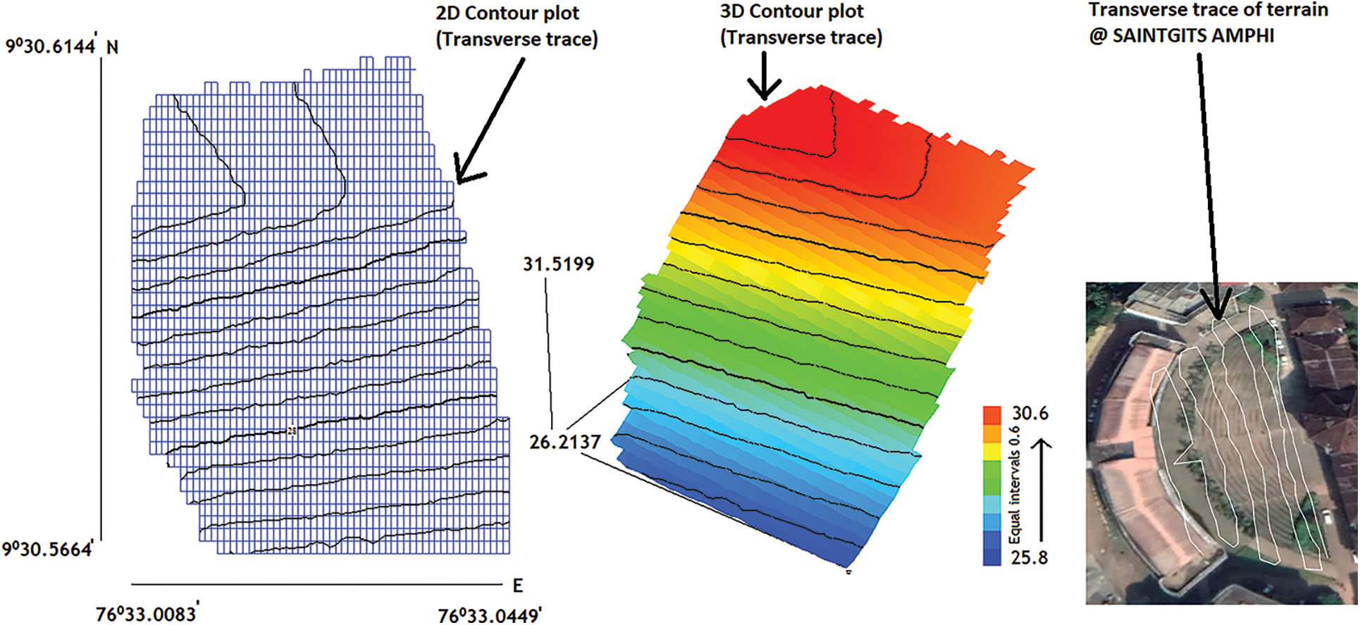
Figure 19: The terrain topology of SAINTGITS AMPHI, measured in the transverse direction, represented as 2D and 3D contour plots

A two-dimensional trace of the longitudinal contour plot had a span of 0.026′ to the East (horizontal) and 0.052′ to the North direction (Vertical). These values make an approximate linear measurement of 38 and 96 m in the East and North directions, respectively. The physical unerring measurements of the amphitheatre at SAINTGITS are 39.5 m to East and 86 m to North. Hence, the decoded values from GEP had been validated with the real measurements. A three-dimensional plot of the contour had the altitude varying from 25.95 to 31.26 m (5.3 m) (Fig. 18).

In the case of the transverse trace, the resultant altitude was found to be at par with the value of the longitudinal contour plot (5.3 m). The values in the East and North directions were 53.62 and 88.85 m, respectively (Fig. 19).

An overall analysis reiterates the robustness of the GEP data, irrespective of the direction of the contour plot (Figs. 18 and 19). The terrain over SAINTGITS AMPHI had a modest gradient within an altitude difference of 5.3 m. Hence, the twelve stair amphitheatre possesses all the essential attributes to christen it as an iconic natural terrain within the SAINTGITS campus to host live acoustic performances.

A set of orthographic projections were developed to visually analyse the altitude gradient of longitudinal and transverse plots (Fig. 20). The plots on the YZ plane depict the altitude gradient, a prime attribute of any amphitheatres worldwide.

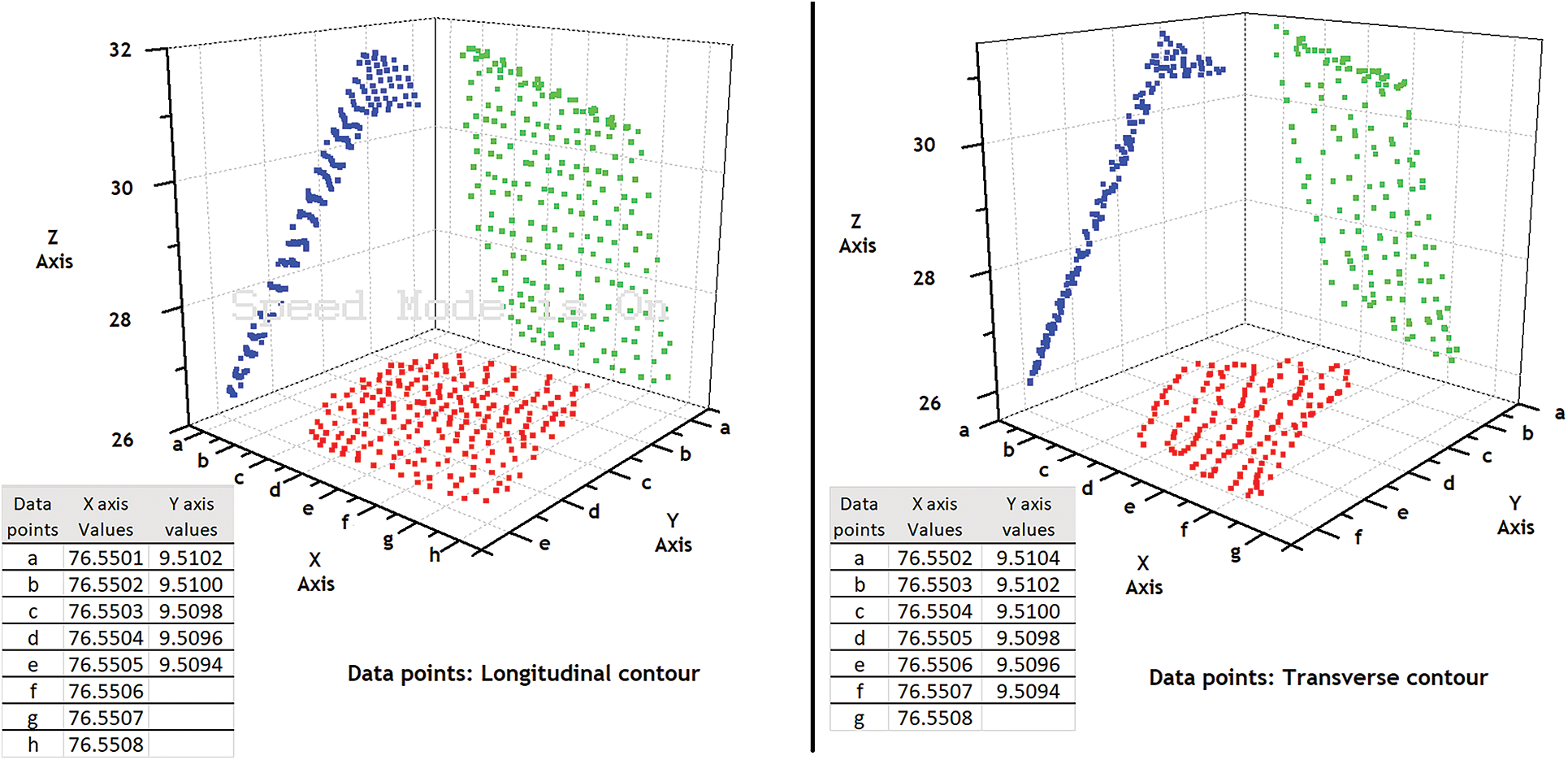
Figure 20: A comparison of Longitudinal and transverse trace: Orthographic projection of the contour plots on XY, YZ and XZ planes to reaffirm the independence of terrain gradient (YZ plot)

Whilst a stark comparison recapitulates the similarity of altitude gradient in both longitudinal and transverse plots, beyond any iota of doubt, these orthographic projections summarize the independence of the projected terrain gradient on the YZ plane. To remain specific, the orthographic projection of terrain gradient obtained on the XZ plane does not depend on the number of data points and the direction of plot progress (Fig. 20). Since the propagation of sound over non-flat terrains behaves differently, the previous session (see Session 3.4) has realistically incorporated the altitude variance at each of the twelve stairs of SAINTGITS AMPHI.

4  Conclusion

An exclusive analysis of the acoustic characteristics and the comparison of terrain topography at the naturally carved landmark of SAINTGITS have revealed promising results that would certainly benefit the sound designers and event managers at all levels. This work has addressed both the recreation aspects and technical know-how of airborne acoustic transmission over SAINTGITS AMPHI. In a nutshell, it is encouraged to interpret the values of Sound Pressure Level as audience-centric (A-Weighting) than source-centric (Z-Weighting). This piece of research also reiterates the significance of beam angle. Among the modest range of beam angles analysed in this manuscript, a vertical beam angle of −4.0° was found to deliver the richness of any live performances at SAINTGITS AMPHI. Since the airborne sound transmission is a function of the surface textural attributes, meteorological conditions and terrain topography, the contour plots were traced for two distinct patterns. A visual inspection of the orthographic projection reaffirms that the terrain gradient (YZ plot) is independent of the direction of plot progress (longitudinal progress or transverse progress). To conclude, this work constructively exploited the immense research potential of the freeware: CADMAPPER, QUICKGRID and EASE Focus. Since sustainable practices are always at the forefront, let this research enlighten the practicing engineers and budding architects trans world.

Funding Statement: This research is funded and supported by the Centre for Engineering Research and Development under the Research Seed Money scheme (CERD-RSM 2018 No. ME02 KTU/Research 2/3894/2018) of APJ Abdul Kalam Technological University, Thiruvanathapuram, Kerala State, India.

Conflicts of Interest: The authors declare that they have no conflicts of interest to report regarding the present study.

References

1. Dennis, J. G. (1972). Structural geology. New York: Ronald Press Company. [Google Scholar]
2. Clark, D., Reynolds, S., Lemanowski, V., Stiles, T., Yasar, S. et al. (2008). University students’ conceptualization and interpretation of topographic maps. International Journal of Science Education, 30(3), 377–408. DOI 10.1080/09500690701191433. [Google Scholar] [CrossRef]
3. Rapp, D. N., Culpepper, S. A., Kirkby, K., Morin, P. (2007). Fostering students’ comprehension of topographic maps. Journal of Geoscience Education, 55(1), 5–16. DOI 10.5408/1089-9995-55.1.5. [Google Scholar] [CrossRef]
4. Atit, K., Weisberg, S. M., Newcombe, N. S., Shipley, T. F. (2016). Learning to interpret topographic maps: Understanding layered spatial information. Cognitive Research: Principles and Implications, 1(1), 1–18. DOI 10.1186/s41235-016-0002-y. [Google Scholar] [CrossRef]
5. Geiger, R., Aron, R. H., Todhunter, P. (1995). The influence of topography on the microclimate. In: Geiger, R., Aron, R. H., Todhunter, P. (Eds.The climate near the ground (5th edpp. 327–406, Wiesbaden, Germany: Vieweg+Teubner Verlag. DOI 10.1007/978-3-322-86582-3. [Google Scholar] [CrossRef]
6. Sutherland, L. C. (2000). Overview of outdoor sound propagation. The 29th International Congress and Exhibition on Noise Control Engineering, Nice, France. [Google Scholar]
7. Bolen, L. N., Bass, H. E. (1981). Effects of ground cover on the propagation of sound through the atmosphere. The Journal of the Acoustical Society of America, 69(4), 950–954. DOI 10.1121/1.385618. [Google Scholar] [CrossRef]
8. Attenborough, K., Taherzadeh, S., Bass, H. E. (1995). Benchmark cases for outdoor sound propagation models. The Journal of the Acoustical Society of America, 97(1), 173–191. DOI 10.1121/1.412302. [Google Scholar] [CrossRef]
9. Trikootam, S. C., Hornikx, M. (2019). The wind effect on sound propagation over urban areas: Experimental approach with an uncontrolled sound source. Building and Environment, 149(6), 561–570. DOI 10.1016/j.buildenv.2018.11.037. [Google Scholar] [CrossRef]
10. Long, M. (2014). 2-Fundamentals of acoustics, architectural acoustics (Second Edition), pp. 39–79. Cambridge: Academic Press. [Google Scholar]
11. Ruan, X., Huang, W., Zhang, L., Gao, Y. (2019). Prediction of outdoor noise propagation induced by single-phase power transformers. Sound & Vibration, 53(1), 2–13. DOI 10.32604/sv.2019.04562. [Google Scholar] [CrossRef]
12. Dodge, H. (2014). Amphitheater. In: Smith, C. (Ed.Encyclopedia of global archaeology. New York, NY: Springer. [Google Scholar]
13. Gabucci, A. (2001). The colosseum. Los Angeles, USA: J. Paul Getty Museum. [Google Scholar]
14. Lancaster, L. (2005). The process of building the Colosseum: The site, the materials and the construction techniques. Journal of Roman Archaeology, 18, 57–82. DOI 10.1017/S1047759400007212. [Google Scholar] [CrossRef]
15. Welch, K. (2007). The Roman amphitheatre from its origins to the Colosseum. UK: Cambridge University Press. [Google Scholar]
16. Farnetania, A., Prodi, N., Pompoli, R. (2008). On the acoustics of ancient Greek and Roman theaters. The Journal of the Acoustical Society of America, 124(3), 1557–1567. DOI 10.1121/1.2951604. [Google Scholar] [CrossRef]
17. Chourmouziadou, K., Kang, J. (2008). Acoustic evolution of ancient Greek and Roman theatres. Applied Acoustics, 69(6), 514–529. DOI 10.1016/j.apacoust.2006.12.009. [Google Scholar] [CrossRef]
18. Mourjopoulos, J. (2018). Unravelling the acoustics of ancient amphitheatres, information and communication. https://www.evolving-science.com/information-communication/acoustics-amphitheaters-00739. [Google Scholar]
19. Georgia Institute of Technology (2007). Ancient Greek amphitheater: Why you can hear from back row. ScienceDaily. https://www.sciencedaily.com/releases/2007/04/070404162237.htm. [Google Scholar]
20. Kalaiselvi, R., Ramachandraiah, A. (2016). Honking noise corrections for traffic noise prediction models in heterogeneous traffic conditions like India. Applied Acoustics, 111(1), 25–38. DOI 10.1016/j.apacoust.2016.04.003. [Google Scholar] [CrossRef]
21. Sonaviya, D. R., Tandel, B. N. (2021). Prediction and limitations of noise maps developed for heterogeneous urban road traffic condition: A case study of Surat City, India. Sound & Vibration, 55(1), 57–68. DOI 10.32604/sv.2021.010715. [Google Scholar] [CrossRef]
22. Thomas, S., Herbert, J., Varghese, J. T., Sathish, C. R. K., Quadir, A. et al. (2020). The projected deposition and removal of particulate matter by green façade drapes: A case study at SAINTGITS. IOP Science: Earth and Environmental Science, 489, 012034. DOI 10.1088/1755-1315/489/1/012034. [Google Scholar] [CrossRef]
23. Thomas, S., Herbert, J., Varghese, J. T. (2019). Energy analyses and projected attributes of sustainable retrofits: A case study at SAINTGITS. 2018 IEEE Region 10 Humanitarian Technology Conference (R10-HTC), 1, 1–4. DOI 10.1109/R10-HTC.2018.8629844. [Google Scholar] [CrossRef]
24. Varghese, J. T. (2017). Mass and energy transfer process in high rise green façade structures. Beau Bassin: LAP Lambert Academic Publishing. [Google Scholar]
25. Varghese, J. T., Ghosh, S., Pandey, S., Samanta, R. (2015). Evaluating the cleansing efficiency of an extended living façade draped with Vernonia elaeagnifolia. Journal of Green Building, 10(2), 157–177. DOI 10.3992/jgb.10.2.157. [Google Scholar] [CrossRef]
26. Ishida, K. (1995). Investigation of the fundamental mechanism of the seat-dip effect-Using measurements on a parallel barrier scale-model. Journal of the Acoustical Society of Japan, 16(2), 105–114. DOI 10.1250/ast.16.105. [Google Scholar] [CrossRef]
27. Varghese, J. T., Thomas, S., Herbert, J. (2020). A sustainable green façade retrofit for an iconic built structure: A case study at SAINTGITS. In: Lecture notes in civil engineering, vol. 44, pp. 419–432. DOI 10.1007/978-981-13-9749-3. [Google Scholar] [CrossRef]
28. EASE Focus 3 (2021). https://focus.afmg.eu/index.php/fc-software-en.html. [Google Scholar]
29. Blairon, N., Blanc-Benon, P., Berengier, M., Juve, D. (2001). Calculation of sound propagation over non flat terrain using parabolic equation. 11th International Congress on Acoustics, vol. III. Rome, Italy. ISBN 88–88387–02–01. [Google Scholar]
30. IEC (2017). IEC 61672-2, electroacoustics-sound level meters-pattern evaluation tests. IEC. https://standards.globalspec.com/std/10152641/iec-61672-2. [Google Scholar]
31. Wang, X. (2010). Vehicle noise and vibration refinement, pp. 33–67. Boca Raton, USA; Oxford, England, UK: CRC Press, Woodhead Publishing Limited. [Google Scholar]
32. Kim, G., Han, W. (2018). Sound pressure levels generated at risk volume steps of portable listening devices: Types of smartphone & genres of music. BioMed Central Public Health, 18(1), 481. DOI 10.1186/s12889-018-5399-4. [Google Scholar] [CrossRef]
33. Dolan, T. G., Maurer, J. F. (1996). Noise exposure associated with hearing aid use in industry. Journal of Speech, Language and Hearing Research, 39(2), 251–260. DOI 10.1044/jshr.3902.251. [Google Scholar] [CrossRef]
34. Ajayeoba, A. O., Olanipekun, A. A., Raheem, W. A., Ojo, O. O., Soji-Adekunle, A. R. (2021). Assessment of noise exposure of sawmill workers in Southwest, Nigeria. Sound & Vibration, 55(1), 69–85. DOI 10.32604/sv.2021.011639. [Google Scholar] [CrossRef]
35. Sugiura, Y., Kato, J., Maeda, Y., Iwasaki, M. (2017). A study on frequency response analysis using friction model for frictional systems. IEEE International Conference on Mechatronics (ICM), pp. 37–42. Churchill, VIC. DOI 10.1109/ICMECH.2017.7921077. [Google Scholar] [CrossRef]
36. Attenborough, K. (2007). Sound propagation in the atmosphere. In: Rossing, T. (Ed.Springer handbook of acoustics. Springer Handbooks. New York: Springer. DOI 10.1007/978-0-387-30425-0_4. [Google Scholar]
37. Rakov, D. S., Rakov, A. S., Chursin, Y. A., Pavlichev, V. V., Igumnov, A. O. (2020). High-directional sound propagation over the earth’s surface. Archives of Acoustics, 45(4), 747–752. DOI 10.24425/aoa.2020.135280. [Google Scholar] [CrossRef]
38. Rakov, D. S., Rakov, A. S., Kudryavtsev, A. N., Krasnenko, N. P., Chursin, Y. A. et al. (2019). A study of directional patterns of ultrasonic parametric array. Archives of Acoustics, 44(2), 301–307. DOI 10.24425/aoa.2019.128493. [Google Scholar] [CrossRef]
39. Yamaha-VXL (2021). Advantages of line-array speakers, VXL series. https://usa.yamaha.com/files/download/other_assets/5/1227415/vxl_series_line_array_speakers_e.pdf. [Google Scholar]
40. Geay, T., Michel, L., Zanker, S., Rigby, J. R. (2019). Acoustic wave propagation in rivers: An experimental study. Earth Surface Dynamics, 7(2), 537–548. DOI 10.5194/esurf-7-537-2019. [Google Scholar] [CrossRef]
41. Petrut, T., Geay, T., Gervaise, C., Belleudy, P., Zanker, S. (2018). Passive acoustic measurement of bedload grain size distribution using self-generated noise. Hydrology and Earth System Sciences, 22(1), 767–787. DOI 10.5194/hess-22-767-2018. [Google Scholar] [CrossRef]
Cite This Article
Copyright © 2022 The Author(s). Published by Tech Science Press.
This work is licensed under a Creative Commons Attribution 4.0 International License , which permits unrestricted use, distribution, and reproduction in any medium, provided the original work is properly cited.
Downloads
Citation Tools