Cooperative Angles-Only Relative Navigation Algorithm for Multi-Spacecraft Formation in Close-Range

1  Introduction

Maintaining formation configuration and restructuring control is essential for cooperative spacecraft to accomplish specific missions, and formation control depends on precise relative navigation between the members [1–3]. Estimating based on certain dynamic model, measuring with sensors on the spacecraft, and finally using the EKF filter algorithm or the UKF filter algorithm to update the relative state is the basic framework of the current navigation algorithm [4,5]. Relative dynamic model, the accuracy of on-board sensors together with navigation algorithm affect the accuracy and the observability of relative navigation.

At present, the commonly used sensors for relative measurement of spacecraft formation flying mainly include: relative GPS, microwave radar, LIDAR, visible light camera, infrared camera and laser rangefinder, etc. However, relative navigation based on GPS can be easily interfered by the environment. In addition, members in the formation will lose common star to do the relative measurement if they are far away from each other. Radio ranging navigation has the defect of mirror orbit [6,7]. Angles-only navigation method based on optical camera has the problem of unobservability or weak observability in relative orbit, and the environment in space greatly affects measurement accuracy of the camera [8–10]. In addition, the method that combines radio signals and laser can be applied, which uses the full sky coverage characteristics of radio beams to achieve target orientation, and then guides laser signals to complete distance measurement. However, formation flying of spacecraft often has strict restrictions on the volume and size of measurement equipment and payloads, which requires the use of as few measurement devices as possible to determine the relative orbit.

Range-only measurement via radio signals and angels-only optical navigation devices are relatively simple and reliable in spacecraft formation flying, thus becoming major trend in the field, and lots of research has been conducted by scholars. Dianetti et al. [11] utilized UWB ranging and phase angle difference information to solve the relative spacecraft navigation problem in short-range rendezvous and docking. Woffiden et al. [12] proposed orbital maneuver method to improve angles-only relative navigation system, but frequent orbital maneuvers will cause fuel consumption. Gaias et al. [13] studied the angles-only relative navigation from the perspective of relative orbit elements, and concluded that the semi-major axis of the orbit is not observable. Newman et al. [14] established a second-order nonlinear relative motion equation using QV (Quadratic Volterra) series, thus, to some extent, solved the observability problem of angles-only relative navigation, though the computational complexity is relatively large. Chen et al. [15–17] adopted a cooperative dual-satellite measurement strategy, Gao et al. [18] introduced measurement baseline to solve the observability problem of angles-only relative navigation by adopting dual-camera measurement strategy, which increases hardware cost. Wang et al. [19] solved the unobservability of range-only relative navigation in near-circular orbit by introducing consensus constraints in spacecraft formation, but relative orbit ambiguity problem still exists for angles-only relative navigation.

The main contribution of this paper is to develop a novel consensus constrained relative navigation algorithm for Multi-Spacecraft Formation in Close-Range that based on the lever arm effect of the sensor offset from the spacecraft center of mass, which will avoid angles-only relative navigation algorithm from converging to the mirror orbit. Orbital maneuver and computational burden brought by complex dynamic model are avoided in the proposed method, only single optical camera is needed to realize relative navigation of close-range spacecraft formation flying.

This paper begins with a brief review of Hill-Clohessy-Wiltshire dynamics and camera offset measurement model in Section 2. In Section 3, the consensus constraint model for the relative orbit state is constructed based on which the consensus unscented Kalman filter is designed. In Section 4, the observability analysis of the proposed angles-only relative navigation algorithm is addressed. In Section 5, Monte Carlo simulations with errors and uncertainties are conducted to verify the theoretical results. At last, conclusions are presented in Section 6.

2  Problem Statement and Formulation

2.1 Relative Motion Dynamic

The origin of a rotating local vertical local horizontal (LVLH) reference frame is collocated with the chief spacecraft center of mass. The axes of the LVLH frame are aligned with the chief spacecraft inertial position vector (x axis or radial), the normal to orbit plane (z axis or cross track), and the along-track direction (y axis completes the orthogonal set).

The position and velocity of the deputy spacecraft center of mass relative to the chief center of mass observed from the chief LVLH coordinates is denoted by r(t) and v(t), respectively. Let the relative orbit state is X(t)=[rT,vT]T, the superscript T stands for the operator of transposition. Vectors without a superscript are assumed to be coordinatized in LVLH coordinates.

Then, under the assumptions of two-body problem and the range between the chief and deputy spacecraft is small compared to the radial distance to the center of Earth, the relative motion of the deputy with respect to the chief that is orbiting near-circular can be governed by the well-known Hill-Clohessy-Wiltshire dynamics [20] as follows:

X˙(t)=AX(t)+Bu(t),A=[03×3I3×3KD](1)

where K=diag[3n2,0,−n2],B=[03×3,I3×3]T, D=−2ω×, and ω× is a skew-symmetric matrix representation of the cross product defined by

ω×=[0−n0n00000](2)

where n is the angular velocity of the chief spacecraft. B is the input matrix of control forces u(t)=[ux,uy,uz]T, which is loaded on the deputy along the three axes of LVLH frame. Lastly, I3×3 denotes 3 by 3 identity matrix. The analytic solution of Hill-Clohessy-Wiltshire dynamics for a given initial state can be expressed as follows:

X(t)=Φ(t,t0)X(t0)+∫t0tΦ(τ,t0)Bu(τ)dτ(3)

Φ(t,t0) is the transition matrix from time instance t0 to t, by taking t denoting t−t0 for short, Φ(t,t0) can be given in partition form as follows:

Φ(t,t0)=[ΦrrΦrvΦvrΦvv](4)

Φrr=[4−3cos⁡nt006sin⁡nt−6nt1000cos⁡nt](5)

Φrv=1n[sin⁡nt2−2cos⁡nt02cos⁡nt−24sin⁡nt−3nt000sin⁡nt](6)

Φvr=[3nsin⁡nt006n(cos⁡nt−1)0000−nsin⁡nt](7)

Φvv=[cos⁡nt2sin⁡nt0−2sin⁡nt4cos⁡nt−3000cos⁡nt](8)

2.2 Angles-Only Measurement Model

It is assumed that the origin of the chief-fixed body reference frame is co-located with the chief center of mass. Without loss of generality, an optical-sensor (camera is considered in this work) offset from the chaser center of mass in the chief fixed body frame, i.e., db=[dx,dy,dz]T, is assumed to be fixed. The unit line-of-sight (also named angles-only) measurement can be modeled in the LVLH frame as follows

y=h(r)=r(i)−Cblvlh(i)db‖r(i)−Cblvlh(i)db‖+ε(9)

where ‖⋅‖ is the operator of 2-norm; ε is the line-of-sight measurement noise which is commonly modeled as zero-mean Gaussian noise with the covariance E[ε(k)ε(k)T]=Rk; Cblvlh(i) is the instantaneous body-to-LVLH attitude rotation matrix at time instant ti and assumed to be known for it can be calculated by using the knowledge of inertial attitude, position, and velocity of the chief. It is assumed that the camera measurement frame is aligned with the focal-plane of the camera, and its orientation relative to the chief-fixed body frame is assumed to be a known state. If the chief holds a known attitude relative to the LVLH frame, an alternative expression of measurement model for line-of-sight vector can be governed as follows:

y=h(r)=r(i)−d‖r(i)−d‖+ε(10)

where the assumption of constant attitude could be realized by attitude control which has been demonstrated by D'Amico et al. [21].

3  Relative Orbit Estimation Algorithm

Consider a formation of multiple (at least two) spacecraft, in which the inertial orbit of each spacecraft is assumed to be unknown. Furthermore, it is assumed that each spacecraft installs a directed camera used to measure the line-of-sight relative to other spacecraft and transmits its own estimation to other spacecraft by undirected broadcasting network.

As shown in Fig. 1, there is the distributed measurement and estimation scheme, each spacecraft obtains the measurement and estimate the relative orbit towards another spacecraft in its own LVLH frame. Obviously, if three or more spacecraft are involved in the formation, the relative orbits could form a vector loop which may be used to constrain the estimation. However, the constraint of vector loop would disappeared if only two spacecraft are considered. Then, different estimation method could be designed based on different available information. Thus, these two cases are discussed respectively in the following subsections.

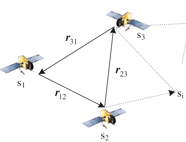
Figure 1: Distributed measurement and estimation scheme where si denotes spacecraft i

3.1 Two-Spacecraft Formation Case

When only two spacecraft are in flight as a formation, there will be no other information except the angles-only measurements could be used to estimate the relative orbit. EKF algorithm is only suitable for the estimation of weakly nonlinear system because it expands the original system and measurement by Taylor series and retains only the linear term. Since the proposed angles-only navigation algorithm represents a nonlinear system, then the UKF introduced by Wan et al. [22] can be utilized to process the measurements for estimation. UKF does not have the linearization process for any nonlinear systems, so it can obtain higher estimation accuracy than EKF. Under the assumption of that the process and measurement noises are purely additive, four steps of the addictive form of UKF algorithm are summarized as follows:

(1)   Initialization

X^0=E[X0](11)

P0=E[(X0−X^0)(X0−X^0)T](12)

(2)   Calculate sigma points and scale weights

χk−1=[X^k−1;X^k−1+n+τ(Pk−1)i;X^k−1−n+τ(Pk−1)i−n](13)

ω0m=τn+τω0c=τn+τ+1−α2+βωim=ωic=12(n+τ),i=1,⋯,2n(14)

τ=α2(n+κ)−n(15)

(3)   Time update

χk|k−1=Φk,k−1χk−1+∫tk−1tkΦ(τ,tk−1)Bu(τ)dτ(16)

X^k−=∑i=02nωimχi,k|k−1(17)

Pk−=∑i=02nωic(χi,k|k−1−X^k−)(χi,k|k−1−X^k−)T+Qk−1(18)

Zk|k−1=H(χk|k−1)(19)

z^k−=∑i=02nωimZi,k|k−1(20)

(4)   Measurement update

Pz^kz^k=∑i=02nωic(Zi,k|k−1−z^k−)(Zi,k|k−1−z^k−)T+Rk(21)

PX^kz^k=∑i=02nωic(χi,k|k−1−X^k)(Zi,k|k−1−z^k−)T(22)

Kk=PX^kz^kPz^kz^k−1(23)

X^k=X^k−+Kk(yk−z^k−)(24)

Pk=Pk−−KkPz^kz^kKkT(25)

where the superscript–marks the priori estimate, Pk is the estimate error covariance matrix.

3.2 Three or More Spacecraft Formation Case

When multiple (at least three or more) spacecraft are involved in the formation, the constraint based on geometrical topology information between spacecraft may be used to improve the estimation. Then, Consensus Unscented Kalman Filter (CUKF) is a good and easy way to utilize the constraint to achieve a better estimation. The key of conducting CUKF to the orbital estimation is to construct the consensus condition. Thus, the consensus would be modeled firstly for the problem and then used in designing CUKF algorithm in the following.

As can be seen from Fig. 1, the position vectors of every three spacecraft are formed a vector loop which naturally is a physical constraint on the orbit estimations. From the viewpoint of observability, the observability of a system improves whenever additional constraints are applied on the system [19]. Thus, it is natural and feasible to force the orbit estimations to satisfy this physical constraint for improving the state observability. Further, satisfying the constraint is also a process of achieving consensus between the members of the formation.

Since the distributed estimate strategy is considered, the relative orbit estimations are resolved in different LVLH frames of each spacecraft. Thus, after coordinate transformation, the position vector loop can be expressed as follows:

rij+Cjirjk+Ckirki=0(26)

where i, j, and k are the labels of different spacecraft; rij is the projection of the relative position from spacecraft i to j in the LVLH frame of spacecraft i.

Differentiating on the both side of (26) yields the constraint between the spacecraft velocities

vij+Cjivjk−Cji(Cijωi−ωj)×rjk+Ckivki−Cki(Cikωi−ωk)×rki=0(27)

Then, combing and re-organizing (26) and in matrix form produces

Xij+[Cji03×3−Cji(Cijωi−ωj)×Cjj]Xjk+[Cki03×3−Cki(Cikωi−ωk)×Cki]Xki=0(28)

where Xij is the projection of the relative orbital state from spacecraft i to j in the LVLH frame of spacecraft i, ωi stands for the orbital angular velocity of spacecraft i in the LVLH i frame.

So far, the physical constraint on the relative orbital vectors of the in-loop spacecraft is achieved, which can be used as the consensus condition.

Next, the distributed Consensus Unscented Kalman Filter is considered to be used to estimate the relative orbit for each spacecraft, because of the convergence characteristic of CUKF when smooth and bounded vector field of the dynamics and the measurement are given [23]. According to the theorem of CUKF, all the other steps of CUKF are the same as those of UKF shown in (11)–(25) except the measurement update, as follows:

X^ij=X^ij−+Kij(yij−h(X^ij))−λPij−‖Pij−‖F(X^ij−−X~ij−)(29)

where λ>0 is the consensus feedback gain which have to be chosen carefully to ensure the convergence of consensus [24]. ‖⋅‖F is the operator of Frobenius norm, X~ij− presents the priori estimation in the LVLH i frame under the physical constraint shown in , i.e., X~ij− is calculated from the priori estimation of X^jk− and X^ki− as follows:

X~ij−=−[Cji03×3−Cji(Cijωi−ωj)×Cjj]X^jk−−[Cki03×3−Cki(Cikωi−ωk)×Cki]X^ki−(30)

4  Observability Analysis for Relative Orbit

In this section, the Lie derivative method of the observability analysis for nonlinear systems is introduced, then theoretical observability analysis for the proposed offset camera line-of-sight measurement relative navigation system is presented.

4.1 Lie Derivative Criteria

For a general nonlinear dynamic system defined as

Σ:{x˙=f(x,u)y=h(x)(31)

where x=[x1,x2,…,xn]T∈Rn×1 is the estimated state vector, u=[u1,u2,…,ul]T∈Rl×1 is the input control vector, and y=[y1,y2,…,ym]T∈Rm×1 is the measurement vector, the observability matrix is defined by the nth-order Lie derivatives as

N(x)=∂∂x[Lf0h(x)Lf1h(x)⋮Lfn−1h(x)]∈Rmn×n(32)

where

{Lf0h(x)=h∈Rm×1Lfih(x)=∂Lfi−1h(x)∂xf(x)∈Rm×1(33)

It has been shown that if rank(N)=n, the system is locally observable. According to the theory of local weak observability of nonlinear systems, when the observability matrix composed of low-order Lie derivatives does not satisfy the rank criterion, high-order Lie derivatives in terms of the system must be introduced for analysis until the observability criterion is satisfied. In addition, the system state is unobservable when the recursive Lie derivative does not satisfy the observability rank criterion.

4.2 Observability Analysis

The system state is a 6-dimensional vector, and the observation state is a 3-dimensional unit vector but 2 bearing angles in essence. In order to make the observability matrix potentially full rank, the Lie derivatives are required to calculated at least three times. Without loss of generality, the line-of-sight measurement is adopted to perform the observability analysis of the system. The complex observability matrix is as follows:

N(X)=[K03×3PKHM]∈R9×6(34)

where

K=‖r−d‖2I3×3−(r−d)(r−d)T‖r−d‖3(35)

P=−v(r−d)T‖r−d‖3−(r−d)vT‖r−d‖3−(r−d)TvI3×3‖r−d‖3+3(r−d)(r−d)Tv(r−d)T‖r−d‖5(36)

H=−2vvT‖r−d‖3+6v(r−d)Tv(r−d)T‖r−d‖5−vTvI3×3‖r−d‖3+3(r−d)vTv(r−d)T‖r−d‖5+3(r−d)Tv(r−d)TvI3×3‖r−d‖5+6(r−d)Tv(r−d)vT‖r−d‖5+K‖r−d‖−15(r−d)(r−d)Tv(r−d)Tv(r−d)T‖r−d‖7−(Kr+Dv)(r−d)T‖r−d‖3−(r−d)T(Kr+Dv)I3×3‖r−d‖3−(r−d)(Kr+Dv)T‖r−d‖3−(r−d)(r−d)TK‖r−d‖3+3(r−d)(r−d)T(Kr+Dv)(r−d)T‖r−d‖5(37)

M=−2(r−d)TvI3×3+v(r−d)T‖r−d‖3−2(r−d)vT‖r−d‖3+6(r−d)(r−d)Tv(r−d)T‖r−d‖5+D‖r−d‖−(r−d)(r−d)TD‖r−d‖3(38)

Consider a constant vector c=[c1;c2]∈R6, where ci∈R3,i=1,2. If the homogeneous linear equations Nc=0 in consideration of c only have zero solutions, then the system observability is guaranteed. By expanding Nc=0, we can get

‖r−d‖2I3×3−(r−d)(r−d)T‖r−d‖3c1=0(39)

Pc1+‖r−d‖2I3×3−(r−d)(r−d)T‖r−d‖3c2=0(40)

Hc1+Mc2=0(41)

the relationship between c1 and r−d described in Eq. (39) is

c1=α(r−d)(42)

where α is an arbitrary scalar. Substituting Eq. (42) into Eq. (40) follows:

[‖r−d‖2I3×3−(r−d)(r−d)T‖r−d‖3](c2−αv)=0(43)

therefore, we can infer that

c2=αv+β(r−d)(44)

where β is another scalar. Substituting Eqs. (42) and (44) into Eq. (41) which is the last constraint results

[I3×3‖r−d‖−(r−d)(r−d)T‖r−d‖3][−2βv+βD(r−d)−αKd]=0(45)

similarly, from Eq. (45) we can get

−2βv+βD(r−d)−αKd=η(r−d)(46)

where η is an arbitrary scalar. Put all parameters to the left of equation we have

η(r−d)+β[2v−D(r−d)]+αKd=0(47)

If and only if (r−d), v+ω×(r−d) and v+ω×(r−d), which represents position, velocity and acceleration vector respectively, are not in the same plane, the α=β=η=0 can be inferred. Then we have c1=c2=0 from Eqs. (42) and (44) under the condition of α=β=0, which means the observability matrix is full rank and the system is locally observable. At the same time, a necessary condition for observability can be obtained simply given by

Kd≠0(48)

Eq. (48) tells us that the system is unobservable if d=0 which indicates that the camera offset is not considered. But we must be aware that d≠0 is a necessary but not sufficient condition. For example, when the camera bias is in the direction of along-track, which means d=[0d0]T, the Eq. (48) is still violated.

5  Numerical Simulations

The proposed algorithm is established in MATLAB simulation environment to verify theoretical conclusions mentioned above. The spacecraft parameter settings are shown in Table 1, and UKF filter parameter settings are shown in Table 2. The Hill-Clohessy-Wiltshire dynamics assumes that the chief spacecraft is running in a near-circular orbit. Therefore, the eccentricity settings of the three spacecraft should be small enough, as shown in Table 1 is 0, 0.0002 and 0.0003, respectively. The spacecraft fly in near-earth orbit, and the distance between the members is 1∼7 km, and the perturbation factors such as J2 perturbation and atmospheric drag are not considered in the simulation. Precision of camera angles measurement is set 8.4×10−4rad(0.048∘). The offset of angles-only camera is related to the distance between the spacecraft. As the distance between spacecraft increases, the offset of the camera should also increase accordingly. For the relative navigation of the spacecraft within 10 km, it is more appropriate to set the offset of the camera at 5∼10 m. The consensus feedback coefficient is an optimized value obtained through empirical adjustment, which is set to 0.03 in the simulation.

In order to verify the effectiveness and performance of the proposed algorithm, the following two sets of simulation are performed: in the first group, offset situations are simulated to see whether the relative motion trajectory estimated by the UKF algorithm converges, and in the second group, same offset condition is set to compare convergence performance of CUKF algorithm and UKF algorithm. The statistics of 200 Monte Carlo shooting results are shown in Figs. 2 and 3, the green lines depict the mean estimated error while the red and blue lines describes ±3σ uncertainty boundaries for a 99.973% confidence.

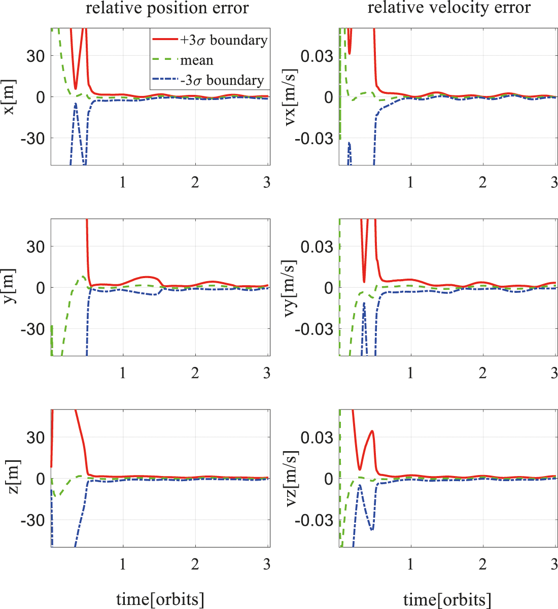
Figure 2: UKF relative position error for X12 when d=[5m,0,0]

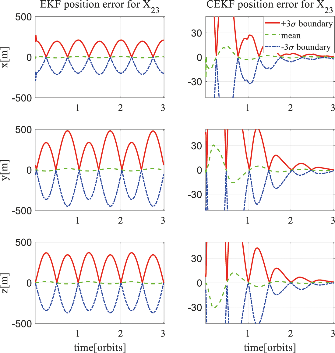
Figure 3: Three-axis position estimation error of X23 under UKF and CUKF filter

5.1 Two-Spacecraft Formation Case

Fig. 2 shows three-axis position and velocity estimation error of the UKF for X12 in consideration of 5 meters camera offset in radius direction. The filter convergence time is half orbit period, and the mean error is close to zero after converging. It can be seen from the left three diagrams that the ±3σ boundary of x-axis position estimation error is 2.1 and −2.5 m, respectively. For y-axis position estimation error, the boundary is 7.6 and −5.1 m. And for z-axis position estimation error, the boundary is 1.4 and −1.5 m. Filter accuracy of y-axis is worse than the other two axes. The three diagrams on the right indicate the relative velocity estimation error. In general, position estimation accuracy is within 10 m and the filtering algorithm is convergent, which proves the feasibility of the proposed off-set camera navigation method.

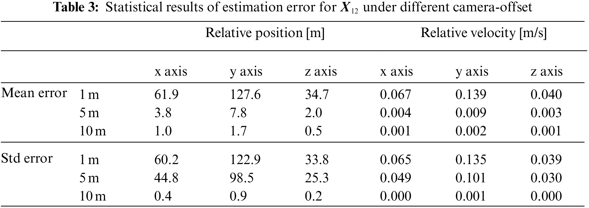
In order to intuitively compare the effects of different camera-offset length on the angles-only relative navigation algorithm proposed in this paper, the following statistics are defined

em(k,t0,t1)=1t1−t0∫t0t1|X^ik(k,t)−Xik(k,t)|dt(49)

where em denotes the average of the absolute value of the difference between the estimated X^ik and the true Xik from t0 when the filter algorithm converges to t1 when the filter algorithm finishes in the k-th Monte Carlo simulation.

Mm(k,t0,t1)=1n∑k=1nem(50)

Pm(k,t0,t1)=1n−1∑k=1n[em−Mm][em−Mm]T(51)

Applying mean error Mm and covariance error Pm, the estimation accuracy and stability of the filter algorithm can be compared. A smaller Mm and Pm indicate a more accurate and stable estimation result. Choosing the filter convergence time t0 as one orbit period, Table 3 shows the estimation error statistical results of the angles-only relative navigation algorithm when camera-offsets are set as 1, 5 and 10 m along the radial direction of the spacecraft orbit, respectively. Taking the x-axis relative position estimation error as an example, the mean errors for 1, 5 and 10 m camera-offset situations are 61.9, 3.8, 1.0 m and the standard deviations are 60.2, 44.8, 0.4 m, respectively. In conclusion, it can be seen from Table 3 that the larger the camera-offset is set, the smaller the mean and standard deviation of the estimation error of the filtering algorithm, thus a more accurate and stable estimation result can be obtained.

5.2 Three or More Spacecraft Formation Case

Suppose the camera offset of the three spacecraft are

d1=[5m,0,0],d2=[0,5m,0],d3=[0,0,5m]

Under such camera offset conditions, combined with the results of the previous observability analysis, we can predict: X23 will converge to the fuzzy orbit under the UKF algorithm, but converges to the true relative orbit under the CUKF algorithm. Fig. 3 shows the position error of X23 using UKF and CUKF. The simulation results are consistent with the prediction. The relative orbit estimated by UKF algorithm converges to fuzzy orbit. But the relative orbit estimated by the CUKF algorithm gradually converges to the true relative orbit at a cost of more convergence time.

6  Conclusions

A new angles-only cooperative relative navigation algorithm for spacecraft formation in close-range is studied in this paper. Based on the Hill-Clohessy-Wiltshire dynamics, this paper studied the convergence of UKF and CUKF when the measurement sensor (camera) is installed offset from the center of mass of the spacecraft. The research work of this paper mainly includes four aspects: (1) The relative motion model between spacecraft and the sensor measurement model with camera installed away from the center of mass are established. (2) The observability of the estimated state is analyzed by introducing the Lie derivative criterion, and the observability conditions of relative position and velocity are obtained. (3) A decentralized estimation strategy based on consistent unscented Kalman filter is designed and the consistent estimation is constructed by using multiple physical constraints. (4) The effectiveness of the algorithm is verified by standard Monte Carlo simulation, and the performance of the algorithm is tested. The results show that for the spacecraft formation with a short distance of 1–7 km, the relative navigation accuracy is within 10 m when 5 m camera offset is designed. The relative navigation algorithm proposed in this paper is based on three spacecraft. When more spacecraft participate in formation or cluster, the decentralized strategy and nonlinear estimation algorithm will be more complex, which will be the main work of future research.

Funding Statement: This work is supported in part by the Natural Science Foundation of China (11802119), Science and Technology on Aerospace Flight Dynamics Laboratory (6142210200306), and Foundation of Science and Technology on Space Intelligent Control Laboratory (6142208200303).

Conflicts of Interest: The authors declare that they have no conflicts of interest to report regarding the present study.

References

 1.  Meng, Y. H. (2014). Introduction to spacecraft formation flying. Beijing, China: Defense Industry Press. [Google Scholar]

 2.  Zhang, H., Gurfil, P. (2018). Cooperative orbital control of multiple satellites via consensus. IEEE Transactions on Aerospace and Electronic Systems, 54(5), 2171–2188. DOI 10.1109/TAES.2018.2808118. [Google Scholar] [CrossRef]

 3.  Zhang, H., Gurfil, P. (2016). Distributed control for satellite cluster flight under different communication topologies. Journal of Guidance, Control, and Dynamics, 39(3), 617–627. DOI 10.2514/1.G001355. [Google Scholar] [CrossRef]

 4.  Ma, G. F., Wang, W., Huang, Q. L., Peng, Y. M., Zhang, X. (2020). Astronomical integrated autonomous navigation method for small thrust orbit change. Journal of Astronautics, 41(9), 1166–1174. DOI 10.3873/j.issn.1000-1328.2020.09.007. [Google Scholar] [CrossRef]

 5.  Alfriend, K. T., Vadali, S. R., Gurfil, P. (2010). Spacecraft formation flying: Dynamics control and navigation. Oxford, UK: Elsevier. [Google Scholar]

 6.  Shi, J. J., Gong, B. C., Li, S., Bai, Y. P., Li, X. (2018). Analytical method of initial relative orbit determination for small satellite proximity operation with range-only measurement. Journal of Astronautics, 39(8), 856–862. DOI 10.3873/j.issn.1000-1328.2018.08.004. [Google Scholar] [CrossRef]

 7.  Gong, B. C., Li, W., Li, S., Ma, W. H., Zheng, L. L. (2018). Angles-only initial relative orbit determination algorithm for non-cooperative spacecraft proximity operations. Astrodynamics, 2, 217–231. DOI 10.1007/s42064-018-0022-0. [Google Scholar] [CrossRef]

 8.  Guo, X. C., Meng, Z. J., Huang, P. F. (2019). State estimation of non-cooperative target stars using monocular vision. Journal of Astronautics, 40(10), 1243–1250. DOI 10.3873/j.issn.1000-1328.2019.10.016. [Google Scholar] [CrossRef]

 9.  Gong, B. C., Li, S., Yang, Y., Shi, J. J., Li, W. D. (2019). Maneuver-free approach to range-only initial relative orbit determination for spacecraft proximity operations. Acta Astronautica, 163(B), 87–95. DOI 10.1016/j.actaastro.2018.11.010. [Google Scholar] [CrossRef]

10. Hu, Y. X., Huang, P. F., Meng, Z. J., Liu, Z. X., Zhang, Y. Z. et al. (2019). Optimal approximation control of space tethered robots with limited vision guidance. Journal of Astronautics, 40(4), 415–424. DOI 10.3873/j.issn.1000-1328.2019.04.006. [Google Scholar] [CrossRef]

11. Dianetti, A. D., Gnam, C., Crassidis, J. L. (2021). Spacecraft proximity operations using ultra-wideband communication devices. AIAA Scitech 2021 Forum. [Google Scholar]

12. Woffinden, D., Geller, D. (2009). Optimal orbital rendezvous maneuvering for angles-only navigation. Journal of Guidance, Control and Dynamics, 32(4), 1382–1387. DOI 10.2514/1.45006. [Google Scholar] [CrossRef]

13. Gaias, G., D'Amico, S., Ardaens, J. (2014). Angles-only navigation to a noncooperative satellite using relative orbital elements. Journal of Guidance, Control and Dynamics, 37(2), 439–451. DOI 10.2514/1.61494. [Google Scholar] [CrossRef]

14. Newman, B., Lovell, A., Pratt, E., Duncan, E. (2015). Hybrid linear-nonlinear initial determination with single iteration refinement for relative motion. 25th AAS/AIAA Space Flight Mechanics Meeting, Williamsburg, USA. [Google Scholar]

15. Chen, T., Xu, S. (2010). Double line-of-sight measuring relative navigation for spacecraft autonomous rendezvous. Acta Astronautics, 67(1–2), 122–134. DOI 10.1016/j.actaastro.2009.12.010. [Google Scholar] [CrossRef]

16. Wang, K., Xu, S. J., Li, K., Tang, L. (2018). Error analysis and formation design for double line-of-sight measuring relative navigation method. Acta Aeronautica et Astronautica Sinica, 39(9), 152–166. DOI 10.7527/S1000-6893.2018.22014. [Google Scholar] [CrossRef]

17. Wang, K., Chen, T., Xu, S. J. (2011). A method of double line-of-sight measurement relative navigation. Acta Aeronautica et Astronautica Sinica, 32(6), 1084–1091. [Google Scholar]

18. Gao, X. H., Liang, B., Pan, L. (2015). High-orbit non-cooperative target multi-line of sight distributed relative navigation method. Journal of Astronautics, 36(3), 292–299. DOI 10.3873/j.issn.1000-1328.2015.03.007. [Google Scholar] [CrossRef]

19. Wang, J., Butcher, E., Tansel, Y. (2019). Space-based relative orbit estimation using information sharing and the consensus kalman filter. Journal of Guidance, Control and Dynamics, 42(3), 491–507. DOI 10.2514/1.G003503. [Google Scholar] [CrossRef]

20. Curtis, H. (2013). Orbital mechanics for engineering students. Elsevier, Ltd., USA. [Google Scholar]

21. D'Amico, S., Ardaens, J. S., Gaias, G. (2013). Noncooperative rendezvous using angles-only optical navigation: System design and flight results. Journal of Guidance, Control and Dynamics, 36(6), 1576–1595. DOI 10.2514/1.59236. [Google Scholar] [CrossRef]

22. Wan, E. A., Van Der Merwe, R. (2000). The unscented Kalman filter for nonlinear estimation. Proceedings of IEEE Adaptive Systems for Signal Processing, Communications, and Control Symposium, pp. 153–158. Alberta. [Google Scholar]

23. Battistelli, G., Chisci, L. (2016). Stability of consensus extended kalman filter for distributed state estimation. Automatica, 68, 169–178. DOI 10.1016/j.automatica.2016.01.071. [Google Scholar] [CrossRef]

24. Olfati-Saber, R. (2010). Kalman-consensus filter: Optimality, stability, and performance. Proceedings of the 48th IEEE Conference on Decision and Control Held Jointly with 2009 28th Chinese Control Conference, pp. 7036–7042. Georgia. [Google Scholar]