Multi-Patch Black-White Topology Optimization in Isogeometric Analysis

1  Introduction

Topology optimization of structures aims to find reasonable material distribution under certain objectives. Combined with Finite Element Method (FEM), by utilizing powerful computational resources, nowadays topology optimization is widely applied for engineering problems. As a new generation of FEM, Isogeometric Analysis (IGA) [1] adopts Non-Uniform Rational B-Spline (NURBS) functions as shape functions. Owing to some conceptual differences between IGA and classical FEM, since then researchers have been studying topology optimization methods in the framework of IGA in many angles.

In 2008, Wall et al. developed a shape optimization strategy by moving control points [2]. In 2010, Youn and his collaborators proposed a topology optimization method using trimming techniques [3,4]. In 2017, Wang et al. focused on lattice materials optimization using asymptotic homogenization schemes [5], then in 2020 Wang and his collaborators proposed a high-efficiency topology optimization method by using multilevel mesh, multi-grid conjugate gradient method and local-update strategy [6]. By transplanting and extending the Moving Morphable Components (MMC) [7], and Moving Morphable Voids (MMV) methods [8], corresponding IGA-based methods were proposed by Hou et al. [9], Xie et al. [10], and Gai et al. [11]. In 2019, Gao et al. conducted the research about isogeometric topology optimization for continuum structures by a constructed density distribution function [12]. For a recent code implementation of topology optimization for structures using IGA in MATLAB, interested readers are referred to [13].

Since in engineer practice a structure model is usually made upon NURBS patches of parts, in this research we mainly study topology optimization of multi-patch IGA, especially in 2D. In FEM framework, Jeong et al. used a condensed mortar method to glue dissimilar interfaces for topology optimization and achieved good performance [14]. In mortar method, the newly introduced corresponding Lagrange multipliers defined along the new interfaces act like forces to enforce the interfaces of both sides to stay tight. The mortar method adds new degrees of freedom (DoFs) into the system, however the newly introduced DoFs can be condensed as in [15]. The mortar method is widely adopted to glue patches in IGA, such as in [15,16]. Usually such a domain decomposition technique can also be used for contact problems, see [17,18], thus the mortar method can also be employed for contact topology optimization [19].

In this paper, we adopt the Nitsche’s method for NURBS patch coupling, by adding external stiffness by multiplying the averaging force and displacement gap along coupling interfaces. The Nitsche’s method introduces no additional DoFs, thus no special treatment is needed for the system, which makes the method suitable for contact problems [20]. Moreover the Nitsche’s method is tested out to be a steady numerical method for patches coupling [21]. In regard to the choice of the topology optimization method, we adopt the sequential integer programming method and Canonical relaxation algorithm proposed by Liang et al. [22]. This method utilizes the sensitivity analysis to construct separable integer programming sub-problems. Besides, Liang et al. proposed the Canonical relaxation algorithm to efficiently solve the integer programming sub-problems. Thanks to the discrete variables, the post-processing treatment to eliminate the gray densities can be avoided. In addition, this method is especially suitable for multi-objective optimization. Combing with the IGA-based methods, the optimized results can be easily parameterized. For further description and code implementation, please refer to [23].

The structure of this paper is organized as follows. In Section 2, the isogeometric multi-patch analysis based on the Nitsche’s method is introduced. In Section 3, we outline the calculation process of the sequential integer programming and discuss the methods for sensitivity filtering and multi-patch treatment. In Section 4, several numerical examples are carried out to show the performance of the proposed method. Conclusions are given in Section 5.

2  Isogeometric Multi-Patch Analysis

2.1 Brief Introduction of IGA

FEM analysis needs two sets of basis functions, one is used for geometry model building, the other one is used for displacement field construction. The main idea of IGA consists in using NURBS as basis functions for both geometry models and the displacement field. The present research mainly focuses on 2D structures, thus only 2D surfaces are introduced, however 3D volumes can be naturally constructed by adding one more dimension.

A 2D surface, denoted by S(ξ,η), can be built by utilization of the NURBS basis functions as Eq. (1)

S(ξ,η)=∑iNi(ξ,η)Pi(x,y),(1)

where Ni(ξ,η) are NURBS basis functions, generated by given sets of knot vectors together with corresponding weights, and Pi(x,y) are called control points.

Following the IGA concept, we approximate the displacement field by Eq. (2)

U(ξ,η)=∑iNi(ξ,η)Ui,(2)

where Ui=(ui,vi)T are nodal displacement degrees of freedom attached to each control point. Note here we use the same set of NURBS basis functions Ni as Eq. (1).

As illustrated in Fig. 1, different from FEM, in IGA the mesh and elements are generated naturally by the given knot vectors, and the elements are usually curved. In addition, in a traditional FEM element, nodes are located on the edges or corners of the element, while in IGA some control points are located outside of the element. For constructing IGA-suitable parameterization for complex CAD models, it is recommended to read [24].

Figure 1: Illustration of the concepts of elements and nodes in FEM(a) and IGA(b)

2.2 The Nitshce’s Method for Multi-Patch Analysis

Consider an interface problem, in which the domain Ω is decomposed into two sub-domains Ωm, where the subscript m=1,2 is used to mark the partitioned domain and corresponding variables. The shared boundary between Ω1 and Ω2 is denoted by Γ, and nm is the unit normal along the interface Γ, pointing out of Ωm. Denote the displacement field to be computed as u:Ω→Rd (d≥1), and denote by v∈V an arbitrary test function that can represent the virtual displacement field, where V is a functional space of admissible fields. Then starting from the original FEM and IGA weak form in Eq. (3)

findu∈V:a(u,v)=L(v),∀v∈V,(3)

by further defining the jump and average operators along the interface Γ in Eq. (4)

[[u]]:=u1−u2,⟨σ(u)⟩:=12(σ1(u)n1−σ2(u)n2),(4)

we finally reach at the weak form of the Nitsche’s method for multi-patch analysis as Eq. (5)

findu∈V:a(u,v)−∫Γ⟨σ(u)⟩[[v]]ds−θ∫Γ[[u]]⟨σ(v)⟩ds+∫Γγ[[u]][[v]]ds=L(v),∀v∈V,(5)

where the θ is named as the Nitsche parameter, and the γ is called the stabilization parameter. The newly added terms are identified as Nitsche’s contribution, in which the second and the third terms are symmetric and they play a key role to glue the two patches, and the forth term is a stabilization term.

The Nitsche parameter θ allows us to select some variants of the Nitsche formulation, that yield different theoretical properties and different degrees of dependency w.r.t. the stabilization parameter γ:

•   for θ=1, the standard symmetric Nitsche’s method is obtained, and a suitable choice for γ is necessary in order to recover well-posedness and optimal accuracy;

•   for θ=0, some terms are canceled and we obtain a simple formulation;

•   for θ=−1, the skew-symmetric Nitsche method is obtained, and it is highlighted that for linear boundary/interface conditions, stability and optimal convergence are ensured even for γ=0, resulting in a parameter-free formulation.

In this research, we set θ=1 to use the standard Nitsche’s method in order to keep the modified system symmetric. For the stabilization parameter γ, we adopt the experienced formula in [25]. For more details about the derivation and theory of the Nitsche’s method, please refer to [20].

From the matrix point of view, imagine we have the original discretized IGA formulation in matrix form, as in Eq. (6)

KU=F,(6)

in which K is the global stiffness matrix, U is the vector of nodal displacement DoFs, and F stands for the nodal force vector. Then assuming we have two NURBS patches to glue, the above formulation can be decomposed as Eq. (7)

[K1K2]=[U1U2][F1F2],(7)

where the subscript stands for the patch index. By pre-defining or other identification techniques, the interface elements are now marked by superscript s and m for interface elements along the two patches respectively. After collecting the indexes of the interface elements, we can rewrite the discretized formulation as Eq. (8)

[K~1K1sK2mK~2]=[U~1U1sU2mU~2][F~1F12F2mF~2],(8)

the tilde means the remaining part, for example K~1=K1−K1s.

As illustrated in Fig. 2, the Nitsche’s method couples the two patches by adding stiffness to the interface elements as Eq. (9)

[K~1K1s+KNssKNsmKNmsK2m+KNmmK~2]=[U~1U1sU2mU~2][F~1F12F2mF~2],(9)

in which the Nitsche related terms can be derived from Eq. (5) as shown in Eq. (10)

KNss=∫Γs−0.5⋅R1Tn1D1B1−0.5⋅B1TD1Tn1TR1+γR1TR1dΓ,KNmm=∫Γs0.5⋅R2Tn1D2B2+0.5⋅B2TD2Tn1TR2+γR2TR2dΓ,KNsm=∫Γs−0.5⋅R1Tn1D2B2+0.5⋅B1TD1Tn1TR2−γR1TR2dΓ,KNms=∫Γs0.5⋅R2Tn1D1B1−0.5⋅B2TD2Tn1TR1−γR2TR1dΓ.(10)

Figure 2: Illustration of the nitsche’s method

In cases of 2D linear elasticity, we have Eq. (11)

R1=[…Ris…],Ris=[NisNis],R2=[…Rim…],Rim=[NimNim](11)

as displacement matrix, and Eq. (12)

B1=[…Bis…],Bis=[∂Nis∂x∂Nis∂y∂Nis∂y∂Nis∂x],B2=[…Bim…],Bis=[∂Nim∂x∂Nim∂y∂Nim∂y∂Nim∂x](12)

as strain-displacement matrix. In addition, D1 and D2 are material constitutive matrix, however in this study we adopt same materials for both sides. Note that the integrations are performed along the slave elements Γs, and n1 is the direction matrix for the strain-displacement adaptation, as in Eq. (13)

n1=[nx0ny0nynx],(13)

where nx and ny are components of vector n1 along x- and y- directions respectively at each quadrature point of the slave interface.

3  Multi-patch IGA Topology Optimization

3.1 Algorithm Description of Sequential Integer Programming

Consider a minimization problem of structural compliance c(p) under material quantity constraint V¯, in the context of pixel (element-wise) description, the optimization formulation is give by Eq. (14)

minρ:c(p)=12UTKUsubject to :∑i=1Nviρi−V¯≤0KU=Pρi∈{0,1},i=1,2…,N,(14)

where the structure is discretized into N elements, each element area is represented by vi. The discrete design variable ρ stands for the element density by taking a value of 0 or 1.

In the algorithm proposed by Liang et al. [22,23], the above problem is first approximated by a series of separable integer programming sub-problems as Eq. (15) show

minρ:∑i=1Nδcδρiρi=∑i=1Nbiρisubject to :∑i=1Nviρi≤V¯ρi∈{0,1}i=1,2…,N,(15)

where the compliance is defined in Eq. (16) as

ce=12UeTKeUe,(16)

and the sensitivity of design variable is defined in Eq. (17) as

δcδρi=bi={−pce,ifρi=1,−pρminp−1ce,ifρi=ρmin.(17)

It should be noted that the density design variable ρ still remains discrete. The relationship between the Young’s modulus and the design variables is assumed to be E=E0ρp, where p is the penalty factor of design variables and it is usually taken as p=3 in common practices. In addition, in order to avoid the singularity of the stiffness matrix due to material reduction, ρmin=10−3 is taken.

After filtering the sensitivities of the design variables from b to b~ using the method described in Subsection 3.2, the series of separable integer programming sub-problems Eq. (15) are solved using the regularized relaxation algorithm. Firstly, the constraints for the discrete design variables ρi are relaxed into the following equality constraints as Eq. (18)

ρi(ρi−1)=0,0≤ρ≤1,i=1,2,…,N.(18)

For Eqs. (15) and (18), define the Lagrangian function as Eq. (19)

L(ρ,λ,σ)=∑i=1Nbiρi+λ(∑i=1Nviρi−V¯)+∑i=1Nσiρi(ρi−1),(19)

where the dual variable λ is introduced for the material quantity constraints, and the dual variable σ is introduced for the equality constraints. Since the Lagrangian function above is differentiable, its first order critical condition in terms of the density variables is given in Eq. (20)

∂L∂ρi=0.(20)

Therefore the original design variable ρi and the two dual design variables λi, σi satisfy the formula

ρi=σi−λvi−b~i2σi,i=1,2,…,N,(21)

which can be simply referred as the original duality relationship. Substitute Eq. (21) into Eq. (19), we get the dual problem of explicit differentiability with any order as the following Eq. (22)

max:Pc(λ,σ)=12∑i=1N(b~i+λvi−σi)24σi−λV¯subject to :λ≥0,σi≥0,i=1,2,…,N.(22)

In order to ensure the above dual problem has critical dual variables that are strictly larger than zero, and thereby to ensure the positive definiteness of the above optimization problem, the objective function of Eq. (22) is perturbed to

Pβc(λ,σ)=12∑i=1N[(b~i+λvi−σi)24σi+σi24β]−λV¯.(23)

Apparently we have limβ→∞⁡Pβc(λ,σ)=Pc(λ,σ). By the convexity and explicit differentiability of Eq. (23), the Karush-Kuhn-Tucker (KKT) conditions for the optimization problem in Eq. (23) can be written as

λ=∑i=1N[(σi−b~i)vi/2σi]−V¯∑i=1N(vi)2/2σi(24)

and

σi3+β2σi2−β2(bi+λvi)2=0,(25)

where β=2×104 is the perturbation parameter.

The presented algorithm is composed by Eqs. (21), (24) and (25). Specifically, the iterative solving process is as follows. In the first step, we initialize the dual variable λ0, and solve for the dual variable σ0 according to the formula Eq. (25). In the next step, the design variable ρi0 is obtained by using the Eq. (21). If a certain convergence criterion is satisfied, it is assumed that approximate integer solutions of the integer programming sub-problems are obtained. Otherwise, we take σ0 into Eq. (24) to get a new dual variable λ1, and the iteration continues.

Due to the integer programming sub-problems are constructed by sensitivity information, the accuracy of these sub-problems is only valid within a local range of current design variables. In order to ensure the approximation accuracy of the integer programming sub-problems, and to make the solutions of the sub-problems converge slowly to the solutions of the original problem, a moving limit strategy should be adopted. Specifically, we gradually reduce the material consumption constraint by a volume fraction reduction factor χ∈[0.95,1). Only when the relative change of the objective function in two adjacent iterations is less than a given value (for example 10−3), the volume fraction can be reduced. Otherwise, it is necessary to continue to iterate at the current volume fraction until the target volume fraction is reached. This strategy is expressed as Eq. (26)

V¯rk+1=max{χV¯rk,V¯},(26)

where rk denotes the number of volume ratio reductions. In this paper, χ=0.98 is taken, which means only 2% of the current volume change is allowed for each iteration loop.

For the present topology optimization technique by the sequential integer programming method, by setting the element density as 1 or 0 in the parameter space, we could achieve a black-white topology design accordingly in the physical space with clear and curved boundaries, as shown in Fig. 3.

Figure 3: Black-white topology optimization in IGA

3.2 Curved Elements Sensitivity filtering by the Helmholtz Equation

In IGA, although the meshes in the parameter space are structured, however the meshes in the physical space are usually curved after mapping. The classical sensitivity filtering technique needs to search adjacent elements and then perform averaging methods, this is not suitable for complex curved meshes in IGA. In this study, the implicit filtering method based on Helmholtz equation [26] is used, which not only saves the amount of calculation effort for searching of adjacent elements, but also ensures the filtering effect. The implicit filtering equation is written as Eq. (27)

KFb~N=TbE,(27)

where bE is the element-wise sensitivity array before filtering, b~N is the node-wise sensitivity array after filtering, and in Eq. (28)

KF=∑e∫Ωe∇ReTKd∇Re+ReTRedΩ(28)

we have the isogeometric stiffness matrix for the scalar problem. Re and ∇Re denote the basis function interpolation matrix and the basis function gradient matrix respectively, symbol ∑ stands for the element stiffness matrix assembly operator. The filter radius rmin controls the range of the filtering circle by Eq. (29)

Kd=[1001]rmin212.(29)

The transformation matrix is given as Eq. (30)

T=∑e∫ΩeReTdΩ,(30)

and it is used for the conversion between element-wise array and node-wise array, for instance in Eq. (31)

bN=TbE,b~E=TTb~N.(31)

Finally, the filtering formula is obtained as Eq. (32)

b~E=TTb~N=TTKF−1TbE.(32)

Note that KF is only related to the original mesh since its generation and remains unchanged in the following topology optimization process, thus KF−1 can be calculated after the mesh initialization, then be utilized repeatedly to save computation resources.

3.3 Multi-Patch Treatment

The flow chart of the discrete variable topology optimization algorithm is drawn in Fig. 4. After the process of IGA analysis with the Nitsche’s method, we obtain a single stiffness matrix K which contains the stiffness contribution of all patches as well as the Nitsche’s coupling. By solving the matrix equation Eq. (6) we reach at U in which the displacements of all the control points of all the patches are listed. According to the sequential integer programming algorithm, the calculation of the compliance ce in Eq. (16) and the following variables are defined and performed element-wisely, thus all the optimization process can be done without considering the multi-patch issue.

Figure 4: Flow chart of the discrete variable topology optimization algorithm

However, for multi-patch sensitivities, since the mesh resolutions of different patches are usually different, the magnitudes of the sensitivity values correspond to meshes of different densities are also different. If these sensitivities are directly substituted into the topology optimization algorithm, it could lead to inappropriate optimization results, especially along the coupling interfaces. In this paper, a simple sensitivity filtering method for the coupling interface is proposed. Suppose that the numbers of elements along both sides of the coupling interface is M1 and M2, and the corresponding sensitivities are b1 and b2, respectively. Refine the meshes on both sides to the same density M, that is, to find the least common multiple of M1 and M2 as Eq. (33)

M=[M1,M2].(33)

Correspondingly, the sensitivities of both sides is scaled as Eq. (34)

b¯1=b1/(M/M1),b¯2=b2/(M/M2).(34)

Since the meshes on both sides are in the same level at this stage, sensitivity filtering can be performed by using a simple averaging method, and the filtered sensitivities b^1 and b^2 can be calculated by, like Eq. (35) for instance

b^1=0.5⋅(b¯1+b¯2),b^2=0.5⋅(b¯1+b¯2).(35)

Finally, the sensitivity is restored to the original meshes by adding all the values within each element

b˜1=∑M1b1^,b˜2=∑M2b2^.(36)

Note that although the relationship between the sensitivities and the mesh resolutions is not linear, we still scale the sensitivities linearly according to mesh refinement by Eq. (34), which does not harm much because in the last step (Eq. (36)) an opposite treatment is performed.

4  Numerical Examples

In the following examples, the material of Young’s modulus E=106 Mpa as well as Poisson’s ratio ν=0.3 are adopted for IGA analysis, and the concentrated force is F=1000 N. For the topology optimization process, it is requited that current volume fraction V¯rk cannot be further reduced until the relative change of the adjacent two objective functions reaches 10−3 or even less. In addition, the sensitivity filter radius rmin is set to be 4 times of the minimum cell length.

4.1 Double-Beam Structure

In order to show the performance of the method in terms of coupling and optimization, and to compare with the existing result of the Mortar method [14], we consider a double-beam structure with overlapped interface as shown in Fig. 5. The beam size is 20 mm × 2 mm, and the two beams are partially overlapped, resulting a shared interface of length 15 mm. The upper beam is meshed into 256×32 elements, and the lower beam is meshed into 512×64 elements. The 60% volume constraint is taken, i.e., V¯=0.6.

Figure 5: The double-beam model

Compute this example using IGA with the Nitsche’s method to glue the overlapped interface, we plot the displacement distribution in Fig. 6, proving the analysis correctness for this example. We reach at the optimization result as shown in Fig. 7. It is noted that in paper [14], two kinds of interface conditions are composed, i.e., tie condition and small sliding condition, since in this paper our objective is to glue both beams by the Nitsche’s method, our results is similar to the optimum results obtained by the interface tie condition, while the small sliding condition is not tested. The stress distribution of the optimized configuration is plotted in Fig. 8, and the iteration history of topology optimization is shown in Fig. 9. This example is also computed by CPS4R elements (4-node bilinear plane stress quadrilateral, reduced integration, hourglass control) using the SIMP optimization method with a penalty coefficient p=3 for design variables. Please note that the result from ABAQUS seems smoother than the proposed result, which is mainly due to the post-processing treatment in ABAQUS, and this could be simply described as drawing black solid lines along the material boundaries. In addition, in order to get a relatively good result as reference, in ABAQUS a well refined mesh is adopted. The objective function values of the configuration by the proposed method shown in Fig. 7 and by ABAQUS shown in Fig. 10 are 382 and 396, respectively, meaning that these two configurations are similar in terms of mechanical characteristics, which once again proves the correctness of the proposed method.

Figure 6: Contour plots of displacement distribution of the double-beam example

Figure 7: Topology optimization result of the double-beam example

Figure 8: Contour plot of Von-Mises stress distribution of the optimized double-beam example

Figure 9: Iteration history of the double-beam example

Figure 10: Topology optimization result by ABAQUS of the double-beam example

Moreover, the curve about the compliance in Fig. 9 appears violent oscillation, which can be explained as follows. In order to ensure the approximation accuracy of the integer programming sub-problems, a volume fraction reduction factor is adopted to gradually reduce the material consumption as a moving limit strategy, as indicated in Eq. (26). Thus the structural compliance is temporarily improved as the material usage is reduced, and the structural compliance is then effectively reduced owing to the proposed optimization algorithm. Until the convergence criterion is reached, the material usage will be once again reduced, and this process is repeated as explained in the flow chart in Fig. 4. Therefore, the value of the object function, i.e., the compliance, appears oscillation unavoidably throughout the iteration history. Although not adopted in this research, this problem could be effectively addressed as reported in paper [27], in which Liang and Cheng proposed a sequential approximate integer programming method with trust region, in order to directly control the amount of the change of the design variables and thus to stabilize the iterative history significantly.

4.2 Cantilever Beam

As the second example, consider the cantilever beam problem as shown in Fig. 11, then verify the results by comparing with the single-patch result and ABAQUS result. The beam size is 100 mm × 50 mm. The cantilever beam is divided into one upper and one lower patches according to the neutral layer, wherein the upper patch is meshed by 128×32 elements, and the lower patch is meshed into 256×64 elements. For better comparison of the effectiveness of the proposed method, the 60% volume constraint, i.e., V¯=0.6 and 50% volume constraint, i.e., V¯=0.5 are both examined.

Figure 11: Cantilever beam model made by two patches

The contour plot of displacement distribution by multi-patch IGA is shown in Fig. 12, indicating that the Nitsche’s method can effectively glue the two patches. The final optimized material distribution is shown in Fig. 13, it can be seen that the material transition at the coupling interface is smooth. The Mises stress distribution is shown in Fig. 14, which shows that the optimized structure is uniformly stressed. The iterative curve of the objective function and material usage is shown in Fig. 15. As the material usage decreases, the structural stiffness decreases, and when the material usage converges to the target volume fraction, the objective function also converges to a stable value.

Figure 12: Contour plots of displacement distribution of the cantilever beam example

Figure 13: Topology optimization results of the cantilever beam example

Figure 14: Contour plots of Von-Mises stress distribution of the optimized cantilever beam example

Figure 15: Iteration histories of the cantilever beam example

In order to illustrate the effectiveness of the proposed method, the result by our method is compared with the results by single patch (Fig. 16), and by ABAQUS (Fig. 17). It can be seen that these two configurations are similar as Fig. 13 by our method. Once again, the result from ABAQUS seems smoother than the proposed result, which is mainly because of its post-processing treatment by drawing solid lines along boundaries as well as the adoption a more refined mesh resolution. The topology optimization results of continuum structures usually depend on mesh generation, thus the density distribution details of these three results are not strictly the same. Furthermore, the values of the objective function correspond to the configurations in Figs. 13–17 are respectively 32.9, 32.1 and 33.9 for V¯=0.6, and 37.6, 35.8 and 38.6 for V¯=0.5. The objective function values of the three configurations are similar, indicating that the mechanical characteristics of the three configurations are similar as well.

Figure 16: Topology optimization results of the cantilever beam example (single patch)

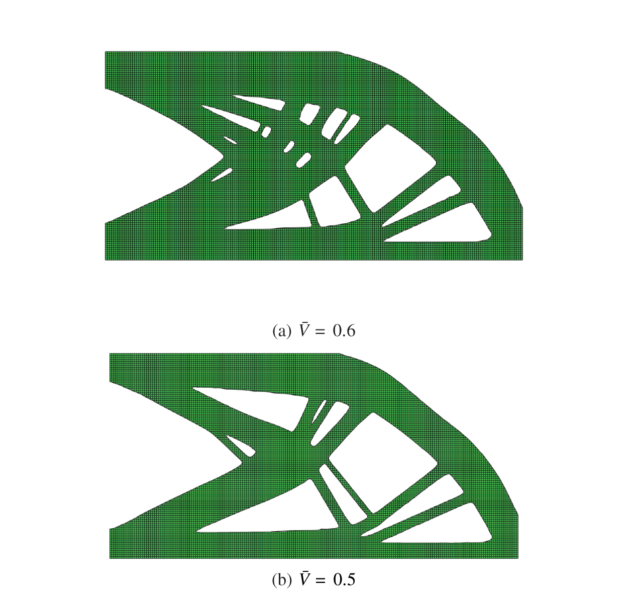
Figure 17: Topology optimization results by ABAQUS of the cantilever beam example

The mathematical nature of the topology optimization problem with discrete variables consists in nonlinear integer programming with partial differential equation constraints, and different discretizations will lead to different local optimal solutions. The method proposed in this paper provides a feasible method for mechanical analysis and topology optimization under different meshes. In practical engineering, structures are usually made upon parts assembling, the advantage of using multi-patches of NURBS models is that it allows engineers to use independent meshes of different parts for analysis and design, which could greatly reduce the mesh requirements.

4.3 One-Quarter Annulus

Finally consider the one-quarter annulus problem as shown in Fig. 18. The model is divided into two patches, and the mesh division is 128×32 and 256×64, respectively. In order to show the advantage of IGA in terms of curved meshes, the two patches are connected by curved edges. Both V¯=0.6 and V¯=0.5 are taken in order to verify the effectiveness of the proposed method.

Figure 18: One-quarter annulus model made by two patches

The displacement distribution of the initial configuration is drawn in Fig. 19, and the final optimized material distribution is shown in Fig. 20. Although the material distribution underthe coarse grid is relatively rough due to the grid resolution of the upper patch, it can be seen that the material transition along the coupling interface is still relatively smooth. It can be inferred that the analysis and optimization method proposed in this paper can effectively deal with the connection of curved interfaces.

Figure 19: Contour plots of displacement distribution of the one-quarter annulus example

The contour plot of the Mises stress is shown in Fig. 21, indicating that the stress distribution of the structure is generally uniform. The iteration curves of the objective function and the material consumption is plotted in Fig. 22. As the material consumption is gradually reduced, the objective function converges to a stable value of 28.2 for V¯=0.6, and 32.2 V¯=0.5. The optimized results by single patch and by ABAQUS are shown in Figs. 23 and 24, the corresponding objective function values are respectively 28.4 and 30.5 for V¯=0.6, and 31.5 and 34.4 for V¯=0.5. By comparing of the optimization results and the objective function values, it is concluded that the obtained optimized configuration in Fig. 20 is effective.

Figure 20: Topology optimization results of the one-quarter annulus example

Figure 21: Contour plots of von-mises stress distribution of the optimized one-quarter annulus example

Figure 22: Iteration histories of the one-quarter annulus example

Figure 23: Topology optimization results of the one-quarter annulus example (single patch)

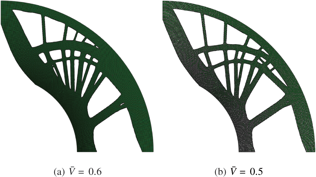
Figure 24: Topology optimization results by ABAQUS of the one-quarter annulus example

5  Conclusions

For multi-patch models in engineer practices, it is necessary to analyze and optimize from the perspective of the entire structure. In this paper, the Nitsche’s method is used to perform the isogeometric multi-patch analysis, which allows the patches of independent meshes to be glued with each other, thus greatly reducing the quality requirements for mesh generation. Furthermore, the discrete topology optimization method based on integer programming is introduced to obtain black-white boundaries of the conceptual design. Taking advantages of curved-edge elements in IGA, topology optimization in the framework of IGA can obtain locally smoother material boundaries than traditional FEM under the same level of mesh resolution. In addition, a sensitivity filtering method based on the Helmholtz equation is used for complex curved-edge elements, which not only ensures the filtering effect, but also saves the computational resources for searching of adjacent elements. In addition, for the coupling interfaces, an averaging method of interface sensitivities is proposed to ensure the transition smoothness of materials. Finally the performance of the proposed method is tested and verified by numerical examples.

It should be noted that although the topology optimization results in this research is totally black and white, the resulting design is still unavoidably jagged due to the nature of the IGA meshes and the nature of the adopted pixel-based element-wise optimization method. However, we believe that the research results have good potential to be adopted as initial configurations for some optimization methods, for instance to provide initial configuration guesses for MMC [7], MMV [8] and the trimmed method [14], and this could be treated as our further research topics.

Acknowledgement: The authors wish to express their appreciation to the reviewers for their helpful suggestions which greatly improved the presentation of this paper.

Funding Statement: Qingyuan HU is supported by the Fundamental Research Funds for the Central Universities (No. JUSRP12038), the Natural Science Foundation of Jiangsu Province (No. BK20200611), and the National Natural Science Foundation of China (No. 12102146).

Conflicts of Interest: The authors declare that they have no conflicts of interest to report regarding the present study.

References

 1.  Hughes, T. J., Cottrell, J. A., Bazilevs, Y. (2005). Isogeometric analysis: CAD, finite elements, nurbs, exact geometry and mesh refinement. Computer Methods in Applied Mechanics and Engineering, 194(39), 4135–4195. DOI 10.1016/j.cma.2004.10.008. [Google Scholar] [CrossRef]

 2.  Wall, W. A., Frenzel, M. A., Cyron, C. (2008). Isogeometric structural shape optimization. Computer Methods in Applied Mechanics and Engineering, 197(33–40), 2976–2988. DOI 10.1016/j.cma.2008.01.025. [Google Scholar] [CrossRef]

 3.  Seo, Y. D., Kim, H. J., Youn, S. K. (2010). Shape optimization and its extension to topological design based on isogeometric analysis. International Journal of Solids and Structures, 47(11–12), 1618–1640. DOI 10.1016/j.ijsolstr.2010.03.004. [Google Scholar] [CrossRef]

 4.  Seo, Y. D., Kim, H. J., Youn, S. K. (2010). Isogeometric topology optimization using trimmed spline surfaces. Computer Methods in Applied Mechanics and Engineering, 199(49–52), 3270–3296. DOI 10.1016/j.cma.2010.06.033. [Google Scholar] [CrossRef]

 5.  Wang, Y., Xu, H., Pasini, D. (2017). Multiscale isogeometric topology optimization for lattice materials. Computer Methods in Applied Mechanics and Engineering, 316, 568–585. DOI 10.1016/j.cma.2016.08.015. [Google Scholar] [CrossRef]

 6.  Wang, Y., Liao, Z., Ye, M., Zhang, Y., Li, W. et al. (2020). An efficient isogeometric topology optimization using multilevel mesh, mgcg and local-update strategy. Advances in Engineering Software, 139, 102733. DOI 10.1016/j.advengsoft.2019.102733. [Google Scholar] [CrossRef]

 7.  Guo, X., Zhang, W., Zhong, W. (2014). Doing topology optimization explicitly and geometrically-a new moving morphable components based framework. Journal of Applied Mechanics, 81(8). DOI 10.1115/1.4027609. [Google Scholar] [CrossRef]

 8.  Zhang, W., Chen, J., Zhu, X., Zhou, J., Xue, D. et al. (2017). Explicit three dimensional topology optimization via moving morphable void (MMV) approach. Computer Methods in Applied Mechanics and Engineering, 322, 590–614. DOI 10.1016/j.cma.2017.05.002. [Google Scholar] [CrossRef]

 9.  Hou, W., Gai, Y., Zhu, X., Wang, X., Zhao, C. et al. (2017). Explicit isogeometric topology optimization using moving morphable components. Computer Methods in Applied Mechanics and Engineering, 326, 694–712. DOI 10.1016/j.cma.2017.08.021. [Google Scholar] [CrossRef]

10. Xie, X., Wang, S., Xu, M., Wang, Y. (2018). A new isogeometric topology optimization using moving morphable components based on r-functions and collocation schemes. Computer Methods in Applied Mechanics and Engineering, 339, 61–90. DOI 10.1016/j.cma.2018.04.048. [Google Scholar] [CrossRef]

11. Gai, Y., Zhu, X., Zhang, Y. J., Hou, W., Hu, P. (2020). Explicit isogeometric topology optimization based on moving morphable voids with closed b-spline boundary curves. Structural and Multidisciplinary Optimization, 61(3), 963–982. DOI 10.1007/s00158-019-02398-1. [Google Scholar] [CrossRef]

12. Gao, J., Gao, L., Luo, Z., Li, P. (2019). Isogeometric topology optimization for continuum structures using density distribution function. International Journal for Numerical Methods in Engineering, 119(10), 991–1017. DOI 10.1002/nme.6081. [Google Scholar] [CrossRef]

13. Gao, J., Wang, L., Luo, Z., Gao, L. (2021). Igatop: An implementation of topology optimization for structures using iga in matlab. Structural and Multidisciplinary Optimization, 64(3), 1669–1700. DOI 10.1007/s00158-021-02858-7. [Google Scholar] [CrossRef]

14. Jeong, G. E., Youn, S. K., Park, K. (2018). Topology optimization of deformable bodies with dissimilar interfaces. Computers & Structures, 198, 1–11. DOI 10.1016/j.compstruc.2018.01.001. [Google Scholar] [CrossRef]

15. Brivadis, E., Buffa, A., Wohlmuth, B., Wunderlich, L. (2015). Isogeometric mortar methods. Computer Methods in Applied Mechanics and Engineering, 284, 292–319. DOI 10.1016/j.cma.2014.09.012. [Google Scholar] [CrossRef]

16. Dornisch, W., Vitucci, G., Klinkel, S. (2015). The weak substitution method–an application of the mortar method for patch coupling in nurbs-based isogeometric analysis. International Journal for Numerical Methods in Engineering, 103(3), 205–234. DOI 10.1002/nme.4918. [Google Scholar] [CrossRef]

17. Kim, J. Y., Youn, S. K. (2012). Isogeometric contact analysis using mortar method. International Journal for Numerical Methods in Engineering, 89(12), 1559–1581. DOI 10.1002/nme.3300. [Google Scholar] [CrossRef]

18. Temizer, I., Wriggers, P., Hughes, T. (2012). Three-dimensional mortar-based frictional contact treatment in isogeometric analysis with nurbs. Computer Methods in Applied Mechanics and Engineering, 209, 115–128. DOI 10.1016/j.cma.2011.10.014. [Google Scholar] [CrossRef]

19. Fernandez, F., Puso, M. A., Solberg, J., Tortorelli, D. A. (2020). Topology optimization of multiple deformable bodies in contact with large deformations. Computer Methods in Applied Mechanics and Engineering, 371, 113288. DOI 10.1016/j.cma.2020.113288. [Google Scholar] [CrossRef]

20. Hu, Q., Chouly, F., Hu, P., Cheng, G., Bordas, S. P. (2018). Skew-symmetric nitsche’s formulation in isogeometric analysis: Dirichlet and symmetry conditions, patch coupling and frictionless contact. Computer Methods in Applied Mechanics and Engineering, 341, 188–220. DOI 10.1016/j.cma.2018.05.024. [Google Scholar] [CrossRef]

21. Apostolatos, A., Schmidt, R., Wüchner, R., Bletzinger, K. U. (2014). A Nitsche-type formulation and comparison of the most common domain decomposition methods in isogeometric analysis. International Journal for Numerical Methods in Engineering, 97(7), 473–504. DOI 10.1002/nme.4568. [Google Scholar] [CrossRef]

22. Liang, Y., Cheng, G. (2019). Topology optimization via sequential integer programming and canonical relaxation algorithm. Computer Methods in Applied Mechanics and Engineering, 348, 64–96. DOI 10.1016/j.cma.2018.10.050. [Google Scholar] [CrossRef]

23. Liang, Y., Cheng, G. (2020). Further elaborations on topology optimization via sequential integer programming and canonical relaxation algorithm and 128-line matlab code. Structural and Multidisciplinary Optimization, 61(1), 411–431. DOI 10.1007/s00158-019-02396-3. [Google Scholar] [CrossRef]

24. Xu, G., Li, M., Mourrain, B., Rabczuk, T., Xu, J. et al. (2018). Constructing iga-suitable planar parameterization from complex cad boundary by domain partition and global/local optimization. Computer Methods in Applied Mechanics and Engineering, 328, 175–200. DOI 10.1016/j.cma.2017.08.052. [Google Scholar] [CrossRef]

25. Hu, Q., Baroli, D., Rao, S. (2021). Isogeometric analysis of multi-patch solid-shells in large deformation. Acta Mechanica Sinica, 37, 844–860. DOI 10.1007/s10409-020-01046-y. [Google Scholar] [CrossRef]

26. Lazarov, B. S., Sigmund, O. (2011). Filters in topology optimization based on helmholtz-type differential equations. International Journal for Numerical Methods in Engineering, 86(6), 765–781. DOI 10.1002/nme.3072. [Google Scholar] [CrossRef]

27. Liang, Y., Sun, K., Cheng, G. (2021). Discrete variable topology optimization for compliant mechanism design via sequential approximate integer programming with trust region (SAIP-TR). Structural and Multidisciplinary Optimization, 64(6), 4441–4441. DOI 10.1007/s00158-021-03083-y. [Google Scholar] [CrossRef]