Bio-Inspired Optimal Dispatching of Wind Power Consumption Considering Multi-Time Scale Demand Response and High-Energy Load Participation

1  Introduction

China's wind power industry keeps a quick increase in recent years. According to the National Energy Bureau data, at December 2019, the country's total wind power installation capacity was 210 million kW, among which three provinces of Xinjiang, Gansu, Inner Mongolia had a capacity of 60.57 million kW [1], accounting for 28.84% of the total installed capacity. However, the problem of wind abandonment in the three provinces is also serious, and the total wind abandonment rate is as high as 28.7% [2]. The issue of blocked wind power consumption has become one of the constraints for the wind power market's expansion in China.

When traditional thermal power units’ peak regulation capability is insufficient to consume wind power completely, using load-side resources to participate in system regulation can provide output space for large-scale integration of wind power [3–6]. Zhang et al. [7] regulates the load through price-based demand response (DR) to actively adjust the system peak and configure the energy storage device at the source side. As a result, the system operation cost is reduced, and the system wind is reduced. Tan et al. [8] combines price-based and incentive DR: it verifies that wind power absorption is significantly increased after the introduction of DR. Tan et al. [9] proposed a two-stage scheduling optimization model, in consideration of DR and energy storage system, to fix the problem by chaotic binary particle swarm optimization algorithm. It revealed that the synergistic effect of DR and energy storage systems could inhibit the uncertainty of wind power and lessen the system's wind curtailment rate. The above literatures have some valuable points in using load-side resources to ease the system's wind curtailment problem.

In July 2020, China's Northwest Power Grid has 14 high-capacity enterprises participating in market regulation, reaching a total peak capacity of 532,000 kW. Therefore, the use of high energy load in the northwest region to attack wind curtailment has certain practical significance [10–12]. Li et al. [13] proposed a ‘source-load’ coordinated scheduling model for high energy load and conventional power supply, which offers a novel approach to solving the issues of wind abandonment. Zhang et al. [14] designed a coordinated scheduling strategy of high-energy load and wind power to take into account the load side's risk constraint to solve the issue of load and wind power mismatch. In reference [15], taking the maximum wind power consumption rate as the objective function, a peak-valley electricity price decision model considering the contribution of high energy load in peak shaving is established to encourage enterprises to take an active role in peak shaving.

The above literature offers a new perspective on the study of high energy load participation in wind power consumption in Northwest China, but there are still the following deficiencies:

(1)   At present, most studies on high energy load only consider a single model rather than modeling it independently based on the high energy load's operation characteristics.

(2)   There is no consideration of the difference in the response speed of different types of high load energy to the dispatching signal.

(3)   The multi-time scale characteristics of high energy load and other demand-side resources are not combined to construct the multi-time scale optimization model of DR to engage in wind power consumption.

For solving the problems of the human real-world, researchers have resorted to nature and biology for a long time. The study of nature theories and principles such as biological structures and bionics bridges have brought development of many mathematical and metaheuristic algorithms by referring to these bio-inspired principles. Bio-inspired modeling researches computerized solutions from living phenomena or biological systems. They have great potential applications in areas such as Internet of Things (IoT) [16–20], Internet of Vehicles (IoV) [21,22], block chain [23–26], image processing [27–31], privacy-preserving [32–34], unmanned aerial vehicles (UAVs) [35–38], medical treatment [39–43] and communication [44,45]. An increasing number of bio-inspired algorithms have been developed in recent decades. Many intelligent algorithms have been adopted recently, such as artificial intelligence algorithms [46–48], the mathematical analytic methods [49–52], ant colonial algorithm [53,54], genetic algorithm [55], particle swarm algorithm, deep learning [56,57] and so forth. Previous studies introduced a mixed-integer linear programming approach to maximize system performance and improve system operational stability [58]. RM et al. [59] proposed an energy efficient cloud algorithm based on Internet of Everything via the wind-driven optimization algorithm and firefly bio-inspired algorithm to handle this heavy flow of data traffic and process within the cloud computing edge. In reference [60], an optimal cluster head strategy is proposed via the employment of a hybrid WOA-MFO model, which optimizes the environmental and network factors. Similarly, the reference [61] designed an advanced approach for cluster head selection through an improved Rider optimization algorithm to optimize the delay minimization, energy sustainability in the IoT system. Neves et al. apply GA to minimize system operation costs in [62], comparing with other algorithms, PSO algorithm is considered more promising in dealing with multi-objective optimization problems. Kerdphol et al. applyed the PSO algorithm to optimize the MG energy storage system [63]. However, the basic PSO algorithm tends to easily fall into a local minimum. Thus, many improvements have been made to solve the disadvantage. To avoid the weaknesses of the PSO algorithm, the acceleration factor is used reasonably to improve the performance of the optimal operation in the power system.

In conclusion, this research examines the principle of high energy load participating in the system to absorb wind power and divides it into discrete adjustable load and continuously adjustable load according to the different operation modes of participating in DR. This study presents an improved bio-inspired algorithm for overcoming the obstruction problem of the large-scale wind power consumption. The main contributions of this work are summarized as follows: (1) The modeling of high energy load based on load characteristics has been designed to show the operation state. (2) The multi-time scale properties of high-energy load and DR are taken into account to minimize the operation cost and maximize the wind power consumption. (3) An improved bio-inspired PSO algorithm has been proposed to overcome the regionally optimal renewable energy power system problem.

2  Load Regulation Characteristics of High Load Energy

2.1 The Principle of High Load Energy-Absorbing Blocked Wind Power

When wind power is at high risk of failure and power generation is constrained, the wind power enterprises can lower the peak-valley difference of equivalent load by coordinating with the high-energy enterprises and adjusting the duration period of high-energy load to improve wind power consumption. High load energy could be used as a resource to absorb wind power specifically in the two aspects as follows:

(1)   With large adjustable capacity, wind power can be absorbed by increasing output when conventional load is low through load transfer.

(2)   The quick response: some high-energy loads can be quickly changed according to the fluctuation of wind power, with a high degree of automation.

In Fig. 1, Region 1 represents the peak regulation range of thermal power units. If the system's initial load curve is superposed with the negative wind power output curve, the system's equivalent load curve can be obtained. The equivalent load PE expression is:

PE=PL−PW(1)

Figure 1: Principal diagram of high load energy accommodating impeded wind power

PL is the system's initial load value when the high load is not involved in regulation; PW represents wind power output.

Region 2 represents the abandoned air volume of the system under the traditional control mode. It is apparent from Fig. 1 that the equivalent load value in t1 − t2 period is smaller than the minimum technical the thermal power unit's output, that is, in this period, the thermal power unit's peak regulation cannot completely suppress the wind power fluctuation, and only the wind power curtailment can be a solution to guarantee the system's operation safety. The abandoned air volume is:

EW=∑t=t1t2(PG,min−PL+PW)Δt(2)

When the high energy load is involved in the regulation and control, the power ΔPH is transferred into the t1 − t2 period, the wind power blocked power will be reduced from Region 2 to Region 3, and the abandoned air volume is:

EW′=∑t=t1t2(PG,min−PL+PW+PH)Δt(3)

Eqs. (2) and (3) shows that the new wind power consumption after high-load energy load participating in regulation is:

Enew=∑t=t1t2PHΔt(4)

Therefore, high load energy regulation can greatly minimize abandoned wind power while also improving the power grid's ability to absorb wind power.

2.2 Regulation Characteristics of High Load Energy

We divide high-energy loads into discrete and continuous types [64].

(1)   Discrete high-energy load is the part that can reduce or increase quantitative load corresponding to the power grid dispatch center's instructions within a given time frame. However, the input or interruption of high-energy load needs a consistently stable period; once the adjustment is carried out, the load power must be maintained for a limited time. It is unable to respond frequently to the adjustment demands, so that is suitable for day-ahead scheduling mode. Take a silicon carbide enterprise as an example. The smelting furnace can be adjusted within the rated capacity range of 80%∼120%, with a sustainable time of 4 h and a discrete adjustment time interval of not less than 1 h.

The formula of the discretely adjustable load is described as:

PDH(t)=∑i=1jth(PDH,i(t−1)+xDH,iΔPDH,i(t))(5)

where t is time, PDH (t) denotes the total load of discretely adjustable load at t. NDH denotes the number of discrete high-energy load units. xDH,i denotes the state variable of the ith discretely adjustable unit, the unit participates in the regulation when the value i is 1. ΔPDH,i is the regulation quantity of discretely adjustable load of the ith unit.

(2)   Continuous high energy load is the part that is continuously adjustable and has no time limit on power retention. This kind of load can be adjusted continuously many times in a certain time range and track wind power fluctuation. Thus, it is suitable for intra-day dispatching mode. Taking one ferroalloy enterprise as an example, its ore heating furnace can be adjusted within the rated capacity range of 90%∼110%, with no strict restriction on adjusting time, and have frequent adjustment and high flexibility.

The formula of the continuously adjustable load is as follows:

PSH(t)=∑j=1NSHxSH,jPSH,j(t)(6)

where PSH (t) denotes the total load of continuously adjustable load at t. NSH denotes the number of continuous high-energy load units. xSH,j denotes the state variable of the jth continuously adjustable unit, the unit participates in the regulation when the value j is 1. PSH,jrepresents the load quantity of continuously adjustable load at t of the jth unit.

3  Multi-Time Scale Model Architecture

3.1 Resource Classification of Demand Response

As discussed above, different kinds of high-energy loads show different response speeds, also for DR resources. There are two kinds of DR resources: price-based demand response (PDR) and incentive demand response (IDR) [65].

PDR refers to users’ change of their electricity demand in reaction to the variation of retail electricity prices. This means a portion of transferable load shifted to the trough stage of electricity price through economic decisions to reduce electricity consumption during peak times. Generally, the user makes the electricity usage plan in accordance with the previous day's price. Therefore, PDR is generally determined in the day-ahead planning.

IDR refers to the DR that the implementation agency encourages users to reply quickly and cut load when system reliability is threatened or at electricity peaks make deterministic or time-varying policies. IDRs can be generally separated into the following two categories [66]:

Class A IDR: Response time is long; scheduling plan have to be made one day in advance and is determined in day-ahead scheduling [67];

Class B IDR: The short response time is determined in the day rolling schedule.

3.2 Multi-Time Scale Framework

Because of the increasing proportion of wind power integration, the traditional day-ahead scheduling method has difficulty solving the wind power consumption problem. Researches show that the multi-time scale scheduling scheme can alleviate the wind curtailment problem greatly [68].

To increase the system's capacity to absorb wind power and lessen operational costs, we design a multi-time scale day-ahead-in-day rolling scheduling model for DR of high load energy participating in wind power accommodation. The scheduling framework is shown in Fig. 2, and the multi-time scale scheduling flow chart is illustrated in Fig. 3.

Figure 2: Multi-time scale framework

Figure 3: Multi-time scale dispatching flow chart

(1)   Day-ahead scheduling plan: It has a time scale of 1 h and an execution cycle of 24 h. Because of the long start-stop time of thermal power units, the start-stop plan should be committed in the day-ahead dispatching. Moreover, PDR response quantity, class A IDR call volume, and discrete high-energy load call volume are supposed to be determined in the day-ahead scheduling. Then, the resource scheduling quantity settled in day-ahead scheduling is considered as the known quantities in intra-day scheduling.

(2)   Intra-day scheduling plan: In day scheduling plan rolls every 15 min [69] and each time for 4 h. The unit output of the first 15 min period is adjusted according to the updated ultra-short-term forecast of wind power and load because the scheduling plan cannot be adjusted repeatedly. The output of the conventional thermal power unit is required to be determined, wind power generation output, IDR call volume of Class B, and continuous high-energy load call volume in the intra-day scheduling.

4  Multi-time Scale Scheduling Model

4.1 Day-Ahead Scheduling Model

4.1.1 Objective Function

The objective function of day-ahead scheduling is to minimize the total operating cost of the system, including thermal power unit operating cost CTh,t, thermal power unit start-stop cost Cqt,t, two types of IDR resource call compensation cost CIDR,t, two types of high-energy load unit switching cost CHE,t, and wind curtailment cost Cqw,t. The relevant formulas are as follows:

f=min∑t=124(CTh,t+Cqt,t+CIDR,t+CHE,t+Cqw,t)=∑t=1NT∑i=1NG[ith(PGi,t)2+biPGi,t+ci]+∑t=1NT∑i=1NGsi(1−ui,t−1)ui,t+∑t=1NT(kIDRA|ΔIDRAt|+kIDRB|ΔIDRBt|)+∑t=1NT∑i=1NDHcDH,iλDH,iΔPDH,i+∑t=1NT∑j=1NSHcSH,jλSH,jΔPDRt,k+∑t=1NTkPDRPqw,t(7)

where NT represents the total number of scheduling periods, the segmented amount of time-of-use electricity price curve, NG represents the total number of conventional units. λt, kPDR is the time-of-use electricity price of PDR at t; PDRt,k represents the response quantity of PDR; ai, bi and ci denote the generation cost coefficients of the ith thermal power unit, respectively; si denotes the start-stop cost coefficient of the ith thermal power unit; ui,t is the running state coefficient of the ith thermal power unit at t, and the value of 1 denotes the running state; PGi,t is the dispatching output of the ith thermal power unit; kIDRA and kIDRB represent the unit invoking cost of class A IDR resource and Class B IDR resource, respectively. ΔIDRAt and ΔIDRBt are the call volumes of class A IDR load and Class B IDR load at t time; cDH,i and cSH,j are the switching costs of discrete-continuous high-energy load units, respectively; λDH,i and λSH,j are the switching stages of discrete high-energy load and continuous high-energy load units, respectively, and the value of 1 denotes that the unit is put into operation, the value of 0 means that the unit is interrupted operation. ΔPDH,i and ΔPSH,j are the switching capacity of discrete high-energy load and continuous high-energy load, respectively; kw represents the wind curtailment penalty cost coefficient; Pqw,t denotes the wind curtailment power at t.

4.1.2 Constraints

(1)   Active power balance constraints:

∑i=1NGPGi,t(t)+Pw(t)=PL(t)+PDH(t)+PSH(t)+ΔPDRt+ΔIDRAt+ΔIDRBt(8)

where Pw(t) represents the wind power output at time t; PL(t) represents the predicted value of load power; PDH(t) represents the operating power of discrete high-energy load after coordinated control optimization. PSH(t) represents the operating power of continuous high-energy load after coordinated control optimization. ΔPDRt is the call volume of PDR.

(2)   The output constraint, climbing constraint and start-stop constraint of thermal power units are respectively referred to formulas (15)–(17) in reference [70].

(3)   Wind turbine output constraints

0≤Pw(t)≤Pwper(t)(9)

(4)   PDR constraints

For the electricity price DR, we select the widely used elastic matrix to calculate the electricity load after participating in the DR. Electricity price elasticity matrix E is obtained by the following formula:

[Δq1q1Δq2q2…Δqmqm]T=E[Δp1p1Δp2p2…Δpmpm]T(10)

The left side of the Equation denotes the load changing rate; the matrix on the right side denotes the electricity price changing rate; E is the elastic matrix, whose main diagonal is the self-elasticity coefficient; the secondary diagonal is the mutual elasticity coefficient.

Upper and lower limit constraints on PDR resource volume are as follows:

ΔPDRt≤λpdrPload,t(11)

where λpdr is the load changing rate of after PDR.

(5)   Upper and lower constraints on IDR resource call volume:

{0≤ΔIDRAt+≤ΔIDRAt+,max0≤ΔIDRAt−≤ΔIDRAt−,max(12)

{0≤ΔIDRBt+≤ΔIDRBt+,max0≤ΔIDRBt−≤ΔIDRBt−,max(13)

(6)   The scheduling constraints of discretely adjustable high-energy load [71]:

1.   Total load conservation constraints:

PDH,i0=∑t=1TPDH,i′(t)(14)

The initial total load of discretely adjustable load i before scheduling; represents the quantity of discretely adjustable load i after scheduling.

2.   Adjustment range constraints:

ΔPSH,jmin≤PSH(t)−PSH(t−1)≤ΔPSH,jmax(15)

where ΔPSH,jmin and ΔPSH,jmax denote the upper and lower adjust limits of discrete high-energy load, separately.

3.   Response speed constraints

−RSH,jdown≤PSH(t)−PSH(t−1)≤RSH,jup(16)

where, RSH,jup and RSH,jdown are respectively the up and down ramp rates of discrete high-energy load.

4.   Response time interval constraints

λDH,i(t)⋅(λDH,i(t)−λDH,i(t−1))⋅(ΔT∑τ=t−Tg,it−1λDH,i(τ)−TDH,ig)≥0(17)where TDH,ig represents the minimum response time interval of discrete high-energy load. This formula represents that if load i want to change its operating state, it must maintain the same operating state in TDH,ig time before changing.

5.   Response time constraints

0≤∑τ=1T|λDH,i(τ)−λDH,i(τ−1)|≤MDH,i(18)where MDH,i represents the maximum allowable response times of discrete high-energy load i within the scheduling cycle.

(7)   Continuously adjustable high-energy load scheduling constraints

1.   Total load conservation constraints:

PSH,j0=∑t=1TPSH,j′(t)(19)

where PSH,j0 represents the initial total load of continuously adjustable load j before dispatching; PSH,j′(t) denotes the load of continuously adjustable load j after dispatching.

2.   Adjustment range constraints

ΔPSH,jmin≤PSH(t)−PSH(t−1)≤ΔPSH,jmax(20)where ΔPSH,jmin and ΔPSH,jmax are the lower and the upper adjust constraint of continuously adjustable high-energy load j, respectively.

3.   Response speed constraints

−RSH,jdown≤PSH(t)−PSH(t−1)≤RSH,jup(21)

RSH,jup and RSH,jdown are the up and down ramp rates of continued high-energy load.

(8)   Tie-line transmission power constraints

−Ptie,tmax≤Ptie,t≤Ptie,tmax(22)

where Ptie,t is the transmission power of the grid tie-line; Ptie,tmax denotes the transmission power limit of the grid tie-line. Since the transmission power of the grid tie-line is bidirectional, its power limit constraint has positive and negative signs.

4.2 Intra-Day Scheduling Model

4.2.1 Objective Function

The objective function of intra-day scheduling is still the minimum system operation cost, including thermal power unit output cost CTh,t, B class IDR call cost CIDR,t, continuous high-energy load switching cost CSh,t, and wind curtailment cost Cqw,t. Since the start-stop plan of thermal power units, class A IDR call volume and discrete high-energy load call volume have been decided in day-ahead scheduling. Therefore, the start-stop cost of thermal power units, class A IDR calling cost and discrete high-energy load switching cost are constant in day-ahead scheduling and have not been written into the formula.

4.2.2 Constraints

(1)   Active power balance constraints:

f=min∑t=196(CTh,t+CIDR,t+CSH,t+Cqw,t)=∑t=1NT∑i=1NG[ai(PGi,t)2+biPi,t+ci]+∑t=1NTkIDRB|ΔIDRBt|+∑t=1NT∑i=1NSHcSH,iλSH,iPSH,i+∑t=1NTkwPw,t(23)

(2)   The thermal power unit constraints, fan constraints, B type IDR constraints, continuous high load call constraints and tie line transmission power constraints are the same as 4.1.2.

4.3 Optimization Algorithm

Commonly, the optimal operation of a power system can be formulated as a multi-objective or a single-objective function with multi-constraint optimization. The PSO algorithm is suitable for solving multi-objective optimization issues. It is often utilized in the solution of discontinuous and nonlinear problems. However, the basic PSO algorithm tends to result in local minimum. Thus, some improvement has been made to solve the disadvantage. To avoid the disadvantages of the PSO algorithm, the improved PSO method incorporates an inertia weight coefficient into the algorithm modeling, which allows for operational regulation and adjustment of the particles’ flight speed. The PSO has been frequently used to improve the power system optimization procedure in comparison to other algorithms; the PSO achieves a higher level of computation accuracy with fewer repetitions. The flow diagram of the improved PSO is shown in Fig. 4 depicts the stage of optimizing the ultimate outcomes of operation costs.

Figure 4: Flow diagram of the proposed improved PSO

The speed and position update formula in standard particle swarm optimization algorithm is:

vidt+1=ωvidt+c1r1(pidt−xidt)+c2r2(pgdt−xidt)(24)

xidt+1=xidt+vidt+1(25)

where ω means inertia weight,

ω=ωstart−ωstart−ωendtmax×t(26)

where ωstart is the initial inertia weight, ωend is the termination inertia weight, tmax is the maximum number of iterations, and t is the current number of iterations.

The influence of the particle's previous velocity on the current velocity is determined by the inertia weight. By adjusting the inertia weight, the global search ability and local search ability can be coordinated. Eq. (26) is a typical inertia weight decreasing strategy. Under this strategy, the global search ability is strong at the initial stage of iteration. If the best is not obtained at the initial stage, the local search ability will be strengthened with the decreasing, and the search results are easy to fall into the local optimum. Once trapped in the local optimum, it is difficult to jump out. In order to overcome this deficiency, a nonlinear dynamic inertia weight method is proposed in Eq. (27):

ω(t)=ωend+(ωstart−ωend)exp⁡(−k×(ttmax)2)(27)

5  Case Study

5.1 Model Overview

In this study, the improved IEEE-30 node system shown in Fig. 5 is used to simulate the above design strategy. It contains six thermal power units located at nodes 1, 2, 5, 8, 11, and 13, respectively, and a wind power unit with a capacity of 350 MW at node 8. There are one discrete high-energy load unit and two continuous high-energy load units at nodes 4, 7, and 10, respectively. Table 1 displays the operating parameters of each thermal power unit, and Table 2 shows the remaining parameters. Fig. 6 illustrates the time-of-use electricity prices diagram, Figs. 7a–7c demonstrate the total load prediction curve, and Figs. 8a, 8b illustrate the forecasting power output of wind power under positive and reverse peak regulation of wind power.

Figure 5: IEEE-30 system

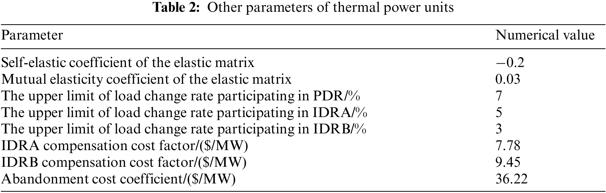
Figure 6: Time-of-use price

Figure 7: (a) The day-ahead and daily load forecasting, (b) The day-ahead and daily wind power forecasting under reverse peak shaving, (c) The day-ahead and daily wind power forecasting under positive peak shaving

Figure 8: (a) Dispatching results under reverse peak regulation of wind power, (b) Dispatching results under positive peak regulation of wind power

5.2 Analysis of Scheduling Results

In both positive and reverse peak regulation scenarios, the results of the proposed scheduling strategy are compared and analyzed in Figs. 8a and 8b.

As demonstrated in Figs. 7 and 9a, 9b, in the reverse-peaking scenario, the high incidence periods of wind power are from 1:00 am to 10:00 am, 11:00 pm–12:00 pm, while the load demand is low at this time. Increasing the load demand at 1:00 am–10:00 am and 11:00 pm–12:00 pm is necessary by calling PDR and IDR to reduce wind curtailment. In the positive peak shaving scenario, the high-frequency period of wind power is between 10 and 19, which overlaps with the load utilization's peak period, and a large amount of wind power can be consumed without large-scale DR resource call. Compared with the peak inversion scenario, the DR resource transfer is reduced by 18.07%.

Figure 9: (a) Transferable energy with DR in the case of reverse peak shaving of wind power, (b) Transferable energy with DR in the case of positive peak shaving of wind power

In addition, although the total amount of transferable load of type B IDR is small, compared with PDR and type A IDR, type B IDR is more flexible and has a faster response speed. Therefore, the change of type B IDR in intra-day scheduling is relatively severe, which is suitable for some sudden situations or the suppression of wind power fluctuations in short time scales.

Figs. 10 and 11 show the calls of discrete high-load and continuous high-load under two wind power scenarios. For the discrete high-load energy load, when the wind power is in the reverse peak trend, the high incidence of wind power is mostly in the morning, so the discrete high-load energy enterprises will transfer part of the 13–24 h load to 1–12 h. When wind power shows a positive peaking trend, high-capacity enterprises will move a portion of the load during the low wind power period to the high wind power period (13:00–24:00). However, such load cannot be continuously regulated in a short time. The call trend for continuous high energy load is roughly the same as that of discrete high energy load in two wind power output scenarios. Moreover, due to its faster response speed, the continuous high load can alleviate the negative impact of large-scale wind power fluctuation in a brief duration in addition to peak load shifting.

Figure 10: Response comparison of discrete high energy load under reverse and positive peak shaving regulation of wind power

Figure 11: Response comparison of continuous high energy load under reverse and positive peak shaving of wind power

In summary, the proposed scheduling policy can fully utilize the time scale characteristics of high load and other DR resources to formulate a reasonable scheduling plan. It helps relieve the issue of wind curtailment and improves the system's economy.

5.3 Comparative Analysis with Different Scheduling Modes

To fully prove that the above scheduling method can efficiently lessen the wind curtailment rate and system's operation cost, we set up the following three different schemes for comparative analysis under two scenarios in which wind power output presents positive and reverse peak regulation, respectively.

Scheduling scheme 1: day-ahead dispatching strategy without participation in system regulation high-energy load.

Scheduling scheme 2: day-ahead dispatching strategy with high-energy load participation in system regulation.

Scheduling scheme 3: adopt the scheduling scheme in this paper.

The scheduling results of scheme 1 are illustrated in Fig. 12. The scheduling results of scheme 2 are illustrated in Figs. 13 and 14. The results of the three schemes are presented in Table 3.

Figure 12: Scheduling results of scheme 1, (a) Scheduling results of wind power with reverse peak regulation, (b) Dispatching results of positive peak of wind power, (c) Demand response resource call in reverse peak regulation of wind power, (d) Demand response resource call when wind power positive peak

Figure 13: (a) Scheduling results of wind power with reverse peak regulation, (b) Dispatching results of the positive peak of wind power

Figure 14: (a) Demand response resource call in reverse peak regulation of wind power, (b) Demand response resource call when wind power positive peak, (c) Response of discrete high load energy load, (d) Response of continuous high energy load

Based on Table 3, a small amount of DR resource calls cannot implement large-scale wind power consumption in scheduling scheme 1, especially under the reverse peak regulation scene in wind power peak time (1–10 h). This leads to serious wind curtailment; the wind curtailment rate reaches up to 12.47%. Therefore, the system reaches the maximum operating cost under this scheme, which is 49,538 dollars.

Based on scheme 1, scheme 2 allows high-energy loads to engage in DR scheduling. Participation of high-energy loads can reduce the system wind curtailment according to the characteristics of high-energy load with large adjustable capacity and convenient control. Compared with plan 1, the wind curtailment rate was reduced by 0.37% and 2.19%, according with the positive and reverse peak regulation scenarios, respectively. As a significant proportion of wind power is consumed, the system wind curtailment cost and thermal power unit output cost are reduced. Compared with Plan 1, the system's operation cost is reduced by 21,233 dollars and 5430 dollars under positive and reverse peak regulation, respectively.

Based on Plan 2, Plan 3 makes full use of the multi-time-scale characteristics of the high-energy load and other DR resources, which can make timely adjustments according to wind power fluctuations in a shorter time scale, and further decrease the wind curtailment rate of the system. The curtailment rate in scheme 3 is reduced by 3.55% and 1.36% under reverse peak regulation and reduced by 1.60% and 1.23% under positive peak regulation, respectively compared with that in schemes 1 and 2. At this time, both the wind curtailment rate and the system operation cost of Scheme 3 is the lowest, with the wind curtailment rate of 1.68% and the system operation cost of 2345 dollars.

To sum up, through the comparative analysis of three different schemes under two scenarios of forward and reverse peak shifting, the efficiency of the scheduling strategy designed in this work is verified for reducing the wind curtailment rate of the system.

6  Conclusion

To address the issues of large-scale wind power consumption and insufficient regulation capacity of traditional units, this paper constructs a bio-inspired computer model by fully exploring the multi-time scale features of DR resources and constructs day-ahead and intra-day rolling scheduling models that include high-energy load in system regulation. The method can obtain the system's optimal scheduling plan. The main conclusions are as follows:

(1)   With the participation of high-energy load, the system's wind power accommodation rate is remarkably increased, and the peak pressure at the source side is effectively decreased. Under the two scenarios of forwarding peak regulation and reverse peak regulation, the system wind power curtailment ratio is decreased by 15.8% in comparison with the traditional scheduling mode.

(2)   The multi-time-scale scheduling model is adopted to make peak-load shifting at the slow response load side resources so that the wind power fluctuations in a short time scale can be suppressed, and the wind power accommodation ability is increased. In addition, the system's operation cost is also lessened due to the decrease of wind power curtailment ratio and the increase of prediction accuracy.

Funding Statement: We would like to express our gratitude to the editors and anonymous reviewers for their comments and suggestions. This research study is supported by the Program for Innovative Research Team (in Science and Technology) in University of Henan Province (No. 22IRTSTHN016) and the Hubei Natural Science Foundation (No. 2021CFB156) and the Japan Society for the Promotion of Science (JSPS) Grants-in-Aid for Scientific Research (KAKENHI) (No. JP21K17737).

Conflicts of Interest: The authors declare that they have no conflicts of interest to report regarding the present study.

References

1. Santoso, H., Nuhung, I. A. (2018). Prospects of renewable energy development within remote or rural areas in Indonesia. In: Transition towards 100% renewable energy. Cham, Springer. DOI 10.1007/978-3-319-69844-1_38. [Google Scholar] [CrossRef]
2. Fox, B., Flynn, D., Bryans, L., Jenkins, N., Milborrow, D. et al. (2007). Wind power integration: Connection and system operational aspects. UK: IET. DOI 10.1049/PBPO050E. [Google Scholar] [CrossRef]
3. Ju, L., Qin, C., Wu, H., He, P., Yu, C. et al. (2015). Wind power accommodation stochastic optimization model with multi-type demand response. Power System Technology, 39(7), 1839–1846. DOI 10.13335/j.1000-3673.pst.2015.07.012. [Google Scholar] [CrossRef]
4. Zhao, C., Wang, J., Watson, J. P., Guan, P. (2013). Multi-stage robust unit commitment considering wind and demand response uncertainties. IEEE Transactions on Power Systems, 28(3), 2708–2717. DOI 10.1109/TPWRS.2013.2244231. [Google Scholar] [CrossRef]
5. Wu, H., Shahidehpour, M., Al-Abdulwahab, A. (2013). Hourly demand response in day-ahead scheduling for managing the variability of renewable energy. IET Generation, Transmission & Distribution, 7(3), 226–234. DOI 10.1049/iet-gtd.2012.0186. [Google Scholar] [CrossRef]
6. Nejad, M. F., Saberian, A. M., Hizam, H., Radzi, M., Kadir, M. (2013). Application of smart power grid in developing countries. 2013 IEEE 7th International Power Engineering and Optimization Conference (PEOCO), Malaysia. DOI 10.1109/PEOCO.2013.6564586. [Google Scholar] [CrossRef]
7. Zhang, X., Yang, X., Wang, H., Liu, K., Zhao, Q. (2018). Study on peaking ability and operation safety of thermal power unit in peak load regulation of power system. 2018 2nd IEEE Conference on Energy Internet and Energy System Integration (EI2), China. DOI 10.1109/EI2.2018.8581889. [Google Scholar] [CrossRef]
8. Tan, Z., Ju, L., Reed, B., Rao, R., Peng, D. et al. (2015). The optimization model for multi-type customers assisting wind power consumptive considering uncertainty and demand response based on robust stochastic theory. Energy Conversion and Management, 105, 1070–1081. DOI 10.1016/j.enconman.2015.08.079. [Google Scholar] [CrossRef]
9. Tan, Z., Ju, L., Li, H., Li, J., Zhang, H. (2014). A two-stage scheduling optimization model and solution algorithm for wind power and energy storage system considering uncertainty and demand response. International Journal of Electrical Power & Energy Systems, 63, 1057–1069. DOI 10.1016/j.ijepes.2014.06.061. [Google Scholar] [CrossRef]
10. Zhu, D., Liu, W., Hu, Y., Wang, W. (2018). A practical load-source coordinative method for further reducing curtailed wind power in China with energy-intensive loads. Energies, 11(11), 2925. DOI 10.3390/en11112925. [Google Scholar] [CrossRef]
11. Yang, X., Guo, G. (2017). Source-load joint multi-objective optimal scheduling for promoting wind power, photovoltaic accommodation. Journal of Renewable and Sustainable Energy, 9(6), 065507. DOI 10.1063/1.4986412. [Google Scholar] [CrossRef]
12. Yu, J., Tao, R., Xia, X., Zhao, D. (2019). Peak load regulation method considering wind power accommodation based on source-load coordination. 2019 IEEE 3rd Conference on Energy Internet and Energy System Integration (EI2), China. DOI 10.1109/EI247390.2019.9061903. [Google Scholar] [CrossRef]
13. Li, W., He, H. (2020). Source-load cooperative optimization dispatch strategy considering wind power accommodation. Power Generation Technology, 41(2), 126–130. DOI 10.12096/j.2096-4528.pgt.18266. [Google Scholar] [CrossRef]
14. Zhang, S., Zhang, K., Zhang, G., Xie, T., Wen, J. et al. (2022). The bi-level optimization model research for energy-intensive load and energy storage system considering congested wind power consumption. Processes, 10(1), 51. DOI 10.3390/pr10010051. [Google Scholar] [CrossRef]
15. Cui, Q., Wang, X., Wang, W. (2015). Stagger peak electricity price for heavy energy-consuming enterprises considering improvement of wind power accommodation. Power System Technology, 39(4), 946–952. DOI 10.13335/j.1000-3673.pst.2015.04.011. [Google Scholar] [CrossRef]
16. Yu, K. (2021). A blockchain-based shamir's threshold cryptography scheme for data protection in industrial Internet of Things settings. IEEE Internet of Things Journal. DOI 10.1109/JIOT.2021.3125190. [Google Scholar] [CrossRef]
17. Tan, L., Shi, N., Yu, K. (2021). A blockchain-empowered access control framework for smart devices in green Internet of Things. ACM Transactions on Internet Technology, 21(3), 1–20. DOI 10.1145/3433542. [Google Scholar] [CrossRef]
18. Wang, D., He, Y., Yu, K. (2021). Delay sensitive secure NOMA transmission for hierarchical HAP-LAP medical-care IoT networks. IEEE Transactions on Industrial Informatics. DOI 10.1109/TII.2021.3117263. [Google Scholar] [CrossRef]
19. Liu, D., Zhang, Y., Wang, W., Dev, K., Khowaja, S. (2021). Flexible data integrity checking with original data recovery in IoT-enabled maritime transportation systems. IEEE Transactions on Intelligent Transportation Systems, 1--12. DOI 10.1109/TITS.2021.3125070. [Google Scholar] [CrossRef]
20. Guo, Z., Yu, K., Jolfaei, A. (2021). Fuz-spam: Label smoothing-based fuzzy detection of spammers in Internet of Things. IEEE Transactions on Fuzzy Systems. DOI 10.1109/TFUZZ.2021.3130311. [Google Scholar] [CrossRef]
21. Zhang, Q., Yu, K., Guo, Z. (2021). Graph neural networks-driven traffic forecasting for connected Internet of Vehicles. IEEE Transactions on Network Science and Engineering, 1--13. DOI 10.1109/TNSE.2021.3126830. [Google Scholar] [CrossRef]
22. Feng, C. (2020). Attribute-based encryption with parallel outsourced decryption for edge intelligent IoV. IEEE Transactions on Vehicular Technology, 69(11), 13784–13795. DOI 10.1109/TVT.2020.3027568. [Google Scholar] [CrossRef]
23. Tan, L., Yu, K., Shi, N. (2022). Towards secure and privacy-preserving data sharing for COVID-19 medical records: A blockchain-empowered approach. IEEE Transactions on Network Science and Engineering, 9(1), 271–281. DOI 10.1109/TNSE.2021.3101842. [Google Scholar] [CrossRef]
24. Lin, X., Wu, J., Mumtaz, S., Garg, S., Guizani, J. (2020). Blockchain-based on-demand computing resource trading in IoV-assisted smart city. IEEE Transactions on Emerging Topics in Computing, 9(3), 1373–1385. DOI 10.1109/TETC.2020.2971831. [Google Scholar] [CrossRef]
25. Wang, W., Xu, H., Alazab, M., Gadekallu, T., Su, C. (2021). Blockchain-based reliable and efficient certificateless signature for IIoT devices. IEEE Transactions on Industrial Informatics, 1551--3203. DOI 10.1109/TII.2021.3084753. [Google Scholar] [CrossRef]
26. Wang, W., Su, C. (2020). CCBRSN: A system with high embedding capacity for covert communication in bitcoin. 35th International Conference on ICT Systems Security and Privacy Protection–IFIP SEC, Slovenia. DOI 10.1007/978-3-030-58201-2_22. [Google Scholar] [CrossRef]
27. Ding, F., Yu, K., Gu, Z., Li, X., Shi, Y. (2021). Perceptual enhancement for autonomous vehicles: Restoring visually degraded images for context prediction via adversarial training. IEEE Transactions on Intelligent Transportation Systems, 1--12. DOI 10.1109/TITS.2021.3120075. [Google Scholar] [CrossRef]
28. Li, H., Zhang, M., Yu, K. (2021). A displacement estimated method for real time tissue ultrasound elastography. Mobile Networks and Applications, 26(3), 1–10. DOI 10.1007/s11036-021-01735-3. [Google Scholar] [CrossRef]
29. Tan, L., Yu, K., Lin, L. (2021). Speech emotion recognition enhanced traffic efficiency solution for autonomous vehicles in a 5G-enabled space-air-ground integrated intelligent transportation system. IEEE Transactions on Intelligent Transportation Systems, 2830--2842. DOI 10.1109/TITS.2021.3119921. [Google Scholar] [CrossRef]
30. Li, H., Zheng, Q., Qi, X. (2021). Neural network-based mapping mining of image style transfer in big data systems. Computational Intelligence and Neuroscience, 1--11. DOI 10.1155/2021/8387382. [Google Scholar] [CrossRef]
31. Guo, T., Yu, K., Aloqaily, M. (2021). Constructing a prior-dependent graph for data clustering and dimension reducton in the edge of AIoT. Future Generation Computer Systems, 381--394. DOI 10.1016/j.future.2021.09.044. [Google Scholar] [CrossRef]
32. Xu, D., Yu, K. (2021). Cross-layer device authentication with quantum encryption for 5G enabled IIoT in Industry 4.0. IEEE Transactions on Industrial Informatics. DOI 10.1109/TII.2021.3130163. [Google Scholar] [CrossRef]
33. Li, H., Yu, K., Liu, B. (2021). An efficient ciphertext-policy weighted attribute-based encryption for the Internet of Health Things. IEEE Journal of Biomedical and Health Informatics. DOI 10.1109/JBHI.2021.3075995. [Google Scholar] [CrossRef]
34. Peng, Y., Jolfaei, A. (2021). A novel real-time deterministic scheduling mechanism in industrial cyber-physical systems for Energy Internet. IEEE Transactions on Industrial Informatics. DOI 10.1109/TII.2021.3139357. [Google Scholar] [CrossRef]
35. Feng, C., Liu, B., Guo, Z. (2021). Blockchain-based cross-domain authentication for intelligent 5G-enabled Internet of Drones. IEEE Internet of Things Journal, 6224--6238. DOI 10.1109/JIOT.2021.3113321. [Google Scholar] [CrossRef]
36. Feng, C., Liu, B., Yu, K. (2021). Blockchain-empowered decentralized horizontal federated learning for 5G-enabled UAVs. IEEE Transactions on Industrial Informatics, 3582--3592. DOI 10.1109/TII.2021.3116132. [Google Scholar] [CrossRef]
37. Ji, B., Li, Y., Cao, D., Li, C., Mumtaz, S. et al. (2020). Secrecy performance analysis of UAV assisted relay transmission for cognitive network with energy harvesting. IEEE Transactions on Vehicular Technology, 69(7), 7404–7415. DOI 10.1109/TVT.2020.2989297. [Google Scholar] [CrossRef]
38. Balamurugan, N., Mohan, S., Adimoolam, M., John, A., Reddy, T. et al. (2022). DOA tracking for seamless connectivity in beamformed IoT-based drones. Computer Standards & Interfaces, 79, 103564. DOI 10.1016/j.csi.2021.103564. [Google Scholar] [CrossRef]
39. Yu, K., Tan, L., Lin, L., Cheng, X. (2021). Deep-learning-empowered breast cancer auxiliary diagnosis for 5GB remote e-health. IEEE Wireless Communications, 28(3), 54–61. DOI 10.1109/MWC.001.2000374. [Google Scholar] [CrossRef]
40. Yang, L., Yu, K., Yang, S. X. (2021). An intelligent trust cloud management method for secure clustering in 5G enabled Internet of Medical Things. IEEE Transactions on Industrial Informatics. DOI 10.1109/TII.2021.3128954. [Google Scholar] [CrossRef]
41. Yu, K., Arifuzzaman, M., Wen, Z. (2015). A key management scheme for secure communications of information centric advanced metering infrastructure in smart grid. IEEE Transactions on Instrumentation and Measurement, 64(8), 2072–2085. DOI 10.1109/TIM.2015.2444238. [Google Scholar] [CrossRef]
42. Tan, L., Yu, K., Bashir, A. K. (2021). Towards real-time and efficient cardiovascular monitoring for COVID-19 patients by 5G-enabled wearable medical devices: A deep learning approach. Neural Computing and Applications, 1--14. DOI 10.1007/s00521-021-06219-9. [Google Scholar] [CrossRef]
43. Sun, Y., Liu, J., Yu, K., Alazab, M., Lin, K. (2021). PMRSS: Privacy-preserving medical record searching scheme for intelligent diagnosis in IoT healthcare. IEEE Transactions on Industrial Informatics, 18(3), 1981–1990. DOI 10.1109/TII.2021.3070544. [Google Scholar] [CrossRef]
44. Zhen, L., Zhang, Y., Yu, K. (2021). Early collision detection for massive random access in satellite-based Internet of Things. IEEE Transactions on Vehicular Technology, 70(5), 5184–5189. DOI 10.1109/TVT.2021.3076015. [Google Scholar] [CrossRef]
45. Zhen, L., Bashir, A. K. (2021). Energy-efficient random access for LEO satellite-assisted 6G Internet of Remote Things. IEEE Internet of Things Journal, 8(7), 5114–5128. DOI 10.1109/JIOT.2020.3030856. [Google Scholar] [CrossRef]
46. Gong, Y., Zhang, L., Liu, R. (2020). Nonlinear MIMO for industrial Internet of Things in cyber–physical systems. IEEE Transactions on Industrial Informatics, 17(8), 5533–5541. DOI 10.1109/TII.2020.3024631. [Google Scholar] [CrossRef]
47. Tan, L., Yu, K., Ming, F. (2021). Secure and resilient artificial intelligence of things: A HoneyNet approach for threat detection and situational awareness. IEEE Consumer Electronics Magazine. DOI 10.1109/MCE.2021.3081874. [Google Scholar] [CrossRef]
48. Tang, Z., Zhao, G., Ouyang, T. (2021). Two-phase deep learning model for short-term wind direction forecasting. Renewable Energy, 2021(173), 1005–1016. DOI 10.1016/j.renene.2021.04.041. [Google Scholar] [CrossRef]
49. Wang, W., Fida M, H., Lian, Z., Yin, Z., Pham, P. Q. et al. (2021). Secure-enhanced federated learning for AI-empowered electric vehicle energy prediction. IEEE Consumer Electronics Magazine. DOI 10.1109/MCE.2021.3116917. [Google Scholar] [CrossRef]
50. Yu, K. (2021). Securing critical infrastructures: Deep-learning-based threat detection in IIoT. IEEE Communications Magazine, 59(10), 76–82. DOI 10.1109/MCOM.101.2001126. [Google Scholar] [CrossRef]
51. Ding, F., Zhu, G., Alazab, M. (2020). Deep-learning-empowered digital forensics for edge consumer electronics in 5G HetNets. IEEE Consumer Electronics Magazine, 11(2), 42–50. DOI 10.1109/MCE.2020.3047606. [Google Scholar] [CrossRef]
52. Yu, K., Guo, Z., Shen, Y. (2021). Secure artificial intelligence of things for implicit group recommendations. IEEE Internet of Things Journal, 9(4), 2698–2707. DOI 10.1109/JIOT.2021.3079574. [Google Scholar] [CrossRef]
53. Shang, L., Tan, L., Yu, K. (2021). Newton-interpolation-based zk-SNARK for artificial Internet of Things. Ad Hoc Networks, 123, 1–11. DOI 10.1016/j.adhoc.2021.102656. [Google Scholar] [CrossRef]
54. Li, H., Zheng, Q., Yan, W. (2021). Image super-resolution reconstruction for secure data transmission in Internet of Things environment. Mathematical Biosciences and Engineering, 18(5), 6652–6671. DOI 10.3934/mbe.2021330. [Google Scholar] [CrossRef]
55. Li, H., Zhang, M., Yu, Z. (2022). An improved pix2pix model based on gabor filter for robust color image rendering. Mathematical Biosciences and Engineering, 19(1), 86–101. DOI 10.3934/mbe.2022004. [Google Scholar] [CrossRef]
56. Li, H., Zheng, Q., Zhang, J., Du, Z. (2021). Pix2pix-based grayscale image coloring method. Journal of Computer-Aided Design & Computer Graphics, 33(6), 929–938. DOI 10.3724/SP.J.1089.2021.18596. [Google Scholar] [CrossRef]
57. Ding, F., Zhu, G., Li, Y., Zhang, X. (2021). Anti-forensics for face swapping videos via adversarial training. IEEE Transactions on Multimedia. DOI 10.1109/TMM.2021.3098422. [Google Scholar] [CrossRef]
58. Toma, L., Tristiu, I., Bulac, C., Neagoe-Stefana, A. (2016). Optimal generation scheduling strategy in a microgrid. IEEE Transportation Electrification Conference and Expo, Asia-Pacific (ITEC), Busan, Korea. DOI 10.1109/ITEC-AP.2016.7513004. [Google Scholar] [CrossRef]
59. RM, S. P., Bhattacharya, S., Maddikunta, P. K. R., Somayaji, S. R. K., Lakshmanna, K. et al. (2020). Load balancing of energy cloud using wind driven and firefly algorithms in Internet of Everything. Journal of Parallel and Distributed Computing, 142, 16–26. DOI 10.1016/j.jpdc.2020.02.010. [Google Scholar] [CrossRef]
60. Maddikunta, P. K. R., Gadekallu, T. R., Kaluri, R., Srivastava, G., Parizi, R. M. et al. (2020). Green communication in IoT networks using a hybrid optimization algorithm. Computer Communications, 159, 97–107. DOI 10.1016/j.comcom.2020.05.020. [Google Scholar] [CrossRef]
61. Alazab, M., Lakshmanna, K., Reddy, T., Pham, Q. V., Maddikunta, P. K. R. (2021). Multi-objective cluster head selection using fitness averaged rider optimization algorithm for IoT networks in smart cities. Sustainable Energy Technologies and Assessments, 43, 100973. DOI 10.1016/j.seta.2020.100973. [Google Scholar] [CrossRef]
62. Neves, D., Pina, A., Silva, C. A. (2018). Comparison of different demand response optimization goals on an isolated MG. Sustainable Energy Technologies and Assessments, 30, 209–215. DOI 10.1016/j.seta.2018.10.006. [Google Scholar] [CrossRef]
63. Kerdphol, T., Fuji, K., Mitani, Y., Watanabem, M., Qudaih, Y. (2016). Optimization of a battery storage system using particle swarm optimization for stand-alone MGs. International Journal of Electrical Power & Energy Systems, 81, 32–39. DOI 10.1016/j.ijepes.2016.02.006. [Google Scholar] [CrossRef]
64. Zhang, Q., Wang, X., Wang, J., Feng, C., Liu, L. (2008). Survey of demand response research in deregulated electricity markets. Automation of Electric Power Systems, 32(3), 97–106. DOI 10.3724/SP.J.1011.2008.00482. [Google Scholar] [CrossRef]
65. Li, Y., Wang, B., Yang, Z., Li, J., Chen, C. (2022). Hierarchical stochastic scheduling of multi-community integrated energy systems in uncertain environments via stackelberg game. Applied Energy, 308, 118392. DOI 10.1016/j.apenergy.2021.118392. [Google Scholar] [CrossRef]
66. Li, Y., Han, M., Yang, Z., Li, G. (2021). Coordinating flexible demand response and renewable uncertainties for scheduling of community integrated energy systems with an electric vehicle charging station: A bi-level approach. IEEE Transactions on Sustainable Energy, 12(4), 2321–2331. DOI 10.1109/TSTE.2021.3090463. [Google Scholar] [CrossRef]
67. Li, Y., Li, K., Yang, Z., Yu, Y., Xu, R. (2022). Stochastic optimal scheduling of demand response-enabled microgrids with renewable generations: An analytical-heuristic approach. Journal of Cleaner Production, 330, 129840. DOI 10.1016/j.jclepro.2021.129840. [Google Scholar] [CrossRef]
68. Cui, Y., Zhang, J., Zhong, W., Wang, Z., Zhao, Y. (2020). Scheduling strategy of wind penetration multi-source system considering multi-time scale source-load coordination. Power System Technology, 2020, 1–11. DOI 10.13335/j.1000-3673.pst.2019.2577. [Google Scholar] [CrossRef]
69. Bao, Y., Wang, B., Li, Y., Yang, S. (2016). Rolling dispatch model considering wind penetration and multi-scale demand response resources. Proceedings of the CSEE, 36(17), 4589–4599. DOI 10.13334/j.0258-8013.pcsee.151343. [Google Scholar] [CrossRef]
70. Li, J., Fu, Y., Li, C., Li, J., Ma, T. (2021). Improving wind power integration by regenerative electric boiler and battery energy storage device. International Journal of Electrical Power & Energy Systems, 131, 107039. DOI 10.1016/j.ijepes.2021.107039. [Google Scholar] [CrossRef]
71. Ge, Y., He, Y., Hu, X., Sun, W., Zhang, W. et al. (2017). Analysis method and empirical research on economic benefit of large-scale consumptive power grid investment. The Journal of Engineering, 2017(13), 1285–1289. DOI 10.1049/joe.2017.0536. [Google Scholar] [CrossRef]
Cite This Article
Copyright © 2023 The Author(s). Published by Tech Science Press.
This work is licensed under a Creative Commons Attribution 4.0 International License , which permits unrestricted use, distribution, and reproduction in any medium, provided the original work is properly cited.
Downloads
Citation Tools