An Efficient Encryption and Compression of Sensed IoT Medical Images Using Auto-Encoder

1  Introduction

Healthcare systems collect data from patients through the Internet of Things (IoT) sensors. The data is then stored in the cloud and analyzed for useful recommendations back to the healthcare provider. However, there are two problems facing the IoT in health systems, especially when such data is spatial: bandwidth congestion and security over the network. This research focuses on using X-ray images as one of the main medical analysis methods for diagnosis. Thus, this research focuses on such data types for health analysis. Healthcare images are huge in size; accordingly, the transmission of such data consumes a lot of bandwidth and thus transmission time. This problem can be reduced by image compression while maintaining resolution, as this data is very sensitive to quality. A major solution to the security issues of health data is encryption. IoT servers are hacked every day [1–3], so encryption of such data is necessary [4,5]. Some models have been developed for image encryption using different algorithms. A chaotic-based artificial neural network (ANN) [6] is a stream image encryption mechanism that has a complex design and is time-consuming. A block-wise pixel shuffling algorithm was proposed for learnable image encryption [7]. A stacked auto-encoder (SAE) network was proposed as an 8-bit RGB image block-wise pixel shuffling algorithm with batch image encryption, which generates two chaotic matrices. One set was used to produce a total shuffling matrix to shuffle the pixel positions on each plain image. The other produced a series of independent sequences, each of which was used to confuse the relationship between the permutated image and the encrypted image. The schema was efficient because of the advantages of parallel computing in SAE, which led to a significant reduction in run-time complexity.

Although the hybrid application of shuffling and confusing enhances the encryption effect, the images still consume transmission overhead, and the process is time-consuming, which is not acceptable. Therefore, image compression also needs to be performed for higher performance. In previous studies [8], an SAE and a chaotic logistic map were suggested for image compression and encryption. Studies have shown that this application is viable and successful. It can be used simultaneously on the internet for picture transmission and safety. A five-layer SAE model was established in which the second layer had fewer neurons than the input layer to realize the primary compression of the image, and the third layer had fewer neurons than the second layer to realize the second stage of the image. The fourth and fifth remaining layers were mirror images of the second and first layers, respectively. In the experiment, the activation function was a nonlinear sigmoid function. The number of neurons was modified to achieve various compression ratios (CRs) in the hidden layers. The model took a lot of time for training and testing due to its complexity. Hence, the present study proposes a simplified and faster model that maintains the intrinsic properties of images. This research has two main contributions. The first one is utilizing the auto-encoder [9,10] for compression. The second is encrypting the X-ray image to secure it during transmission. The auto-encoder is a convolutional neural network used to compress the x-ray image (in the compressing phrase). This step is reversed to get the image decoding. Between the encoding and decoding phases, the output is encrypted and decrypted to secure the image. A classification algorithm is used after using the modified auto-encoder to evaluate the amount of loss in the original image. In this paper, we discuss the effect of the hyperparameter [11] of the auto-encoder on the quality of the retrieved image and the use of an encryption function on image loss. A convolution neural network is also used in the classification algorithm [12,13].

Our approach introduces compression using an auto-encoder and encryption using a customized function that is not as complicated as in state-of-the-art models and thus faster. The compression and encryption processes utilize image distortion. Therefore, an artificial application was applied to examine the amount of distortion in the received images. This application was a diagnostic classifier used to examine the acceptable amount of distortion in the images. We also examined different hyperparameters of the modified auto-encoder and assessed their effects on the level of distortion of the images. The contributions of the study are as follows:

1.    An auto-encoder was utilized to compress images to reduce the time taken to transmit them over the internet. After encoding, the feature vector, which was the output of the encoder layer, was encrypted.

2.    After encryption, a reverse function was utilized for the decryption of the feature vector (the output of the encryption function). A mirror reverse of the encoder layers was run on the output of the decryption function to retrieve the original image, with some acceptable loss.

3.    Some changes were made to the auto-encoder hyperparameters to demonstrate their effects on the classification algorithm and the extent of the acceptability of the classification step.

The rest of the paper is organized as follows: Section 2 presents related work. Section 3 introduces the proposed methodology. Section 4 describes the results achieved in this study. The conclusions are drawn in Section 5.

2  Related Work

IoT data security is a very challenging area of research in real life. In this section, a brief discussion of some recent developments in IoT systems, image encryption, and auto-encoders is presented. Hu et al. [14] proposed a batch image encryption scheme that included a stacked auto-encoder. The SAE network was introduced to create two chaotic matrices. One set was used to create a complete shuffling matrix to shuffle the pixel positions on every image. Another set generated a series of separate sequences, each of which was used to confuse the relationship between the permutated image and the encrypted image. The framework was efficient because of the benefits of SAE’s parallel computing, which led to a substantial decrease in its complexity. The hybrid implementation of shuffling and confusing improved the encryption effect. The authors contrasted the model with the prevalent “logistic diagram” to determine the efficacy of the system, and the performance in running time estimation was collected. The results and review of the experiments showed that their device had a strong encryption effect and was capable of resisting brute force, statistical, and differential attacks.

Thanikaiselvan et al. [15] suggested implementing a batch image encryption method using a stacked auto-encoder network in which two chaotic sequences were used. The first sequence shuffles the image pixels of each input image, creating a shuffling matrix. The other sequence generates a set of separate sequences that are used to confuse the allowed images with the encrypted images. Parallel computation of the stacked auto-encoder in this scheme could reduce the complexity of the run time and improve the encryption effect. A collection of studies has assessed the performance of the scheme and concluded that the proposed scheme is capable of avoiding statistical and differential attacks. Sushmit et al. [16] presented a method of X-ray image compression based on a recurrent neural network convolution (RNN-Conv). During implementation, the proposed architecture can provide variable compression rates, while requiring each network to be trained only once for a particular X-ray image dimension. For efficient compression, the model uses a multi-level pooling scheme that learns contextualized features. Using the National Institute of Health (NIH)’s Chest X-ray dataset, they conducted image compression experiments and compared the output of the proposed architecture with a state-of-the-art RNN-based technique and JPEG 2000. In terms of the structural similarity index (SSIM) and peak signal-to-noise ratio (PSNR) metrics, the experimental results reflected improved compression efficiency.

Akyazi et al. [17] introduced a learning-based method of image compression using wavelet decomposition as a preprocessing stage. The proposed convolution auto-encoder was trained end-to-end to achieve a target bit rate of less than 0.15 bits per pixel across the entire CLIC2019 test range. The proposed model outperformed legacy JPEG compression as well as an auto-encoder of a related convolution that lacks the proposed preprocessing. The presented architecture demonstrates that wavelet decomposition is useful in modifying the compressed image’s frequency characteristics and helps enhance the performance of image compression models based on learning. Optimization of wavelet scales at the analysis/synthesis and quantization stages of the wavelet convolutional auto-encoders (WCAE) may enhance the implemented method. Vu et al. [18] proposed a new method of representation learning to “describe” unknown attacks more precisely, enabling supervised methods to identify learning-based anomalies. Specifically, to learn a latent representation from the input data, the author created three regularized versions of auto-encoders. The bottleneck layers of these regularized auto-encoders need to be updated in a new classification algorithm. Input features were trained in a controlled way using normal data and known IoT attacks. The authors utilized a supervised learning method for anomaly detection. Specifically, they developed three regularized versions of auto-encoders to learn a latent representation from the input data. They also conducted experiments to explore the features of the proposed models and their effects on the output of the hyperparameters.

Ameen Suhail et al. [19] used an auto-compression encoder and a chaotic encryption logistic map. An auto-encoder is an unsupervised deep-learning neural network algorithm that compresses the input vector into a smaller dimension vector that forms a dense representation of the input data. It is possible to use this feature of the auto-encoder to compress images. The encryption protocol is applied to the compressed data. In shuffling and encrypting the compressed image type, the sequences created by the logistic map are efficiently used. The security review indicates that the device is secure enough for image data to be transmitted. However, the chaotic encryption method is a loosy technique; the output image cannot be returned to its original colors. This is a critical drawback for medical images.

From the previous studies, this research innovation combines two different techniques. The first is to compress medical images with the least amount of image loss. The second is to encrypt the images so they cannot be hacked over the internet, as it is medical data and should be secure. The proposed model combined these two ideas together to show that there is a way that we can send encrypted images with low capacity and minimum loss. To achieve minimum loss, auto-encoder parameters need to be tuned for the best results, which is our main goal in this study. The images need to be regenerated as the originals as soon as possible after transmission, particularly in areas where medical images are used for critical diagnosis. The regenerated images are validated by feeding them into a classifier and verifying the resultant diagnoses.

3  Background and Methodology

Auto-encoders are basic learning circuits aimed at transforming inputs into outputs with the least amount of possible distortion.

Fig. 1 shows auto-encoders that consist of an input layer and an output layer connected by one or more hidden layers. The auto-encoder has two main parts which are responsible for encoding and decoding. The encoding phase is done in the first layers after the input layer. After the encoding phase is ended, some other layers with the same number of the encoding layers are begun but in the inverse structure, which is known as the decoder. The input is obtained by the encoder and converted to a new representation, typically referred to as a code or latent variable. The decoder receives the generated code and converts it to a reconstruction of the original input. The goal of this network is to recreate the input by converting it into outputs in the simplest way possible so that the input is not very distorted. This kind of neural network has been used mostly to solve problems of unsupervised learning as well as transfer learning. An auto-encoder has two main components: an encoder and a decoder. The training method for auto-encoders requires minimizing reconstruction errors; that is, the output and input must differ as little as possible [20]. The standard AE structure is shown in Fig. 1.

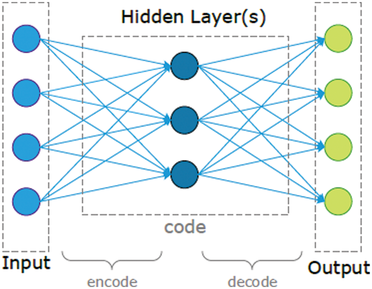
Figure 1: Structure of auto-encoders

To compress an image, the AE has some nodes in the hidden layer that is less than the number of pixels in the input layer. The code produced by the hidden layer is transmitted to the other side. The received code is decoded into the original image through the output layer, which has the same number of nodes as the input layer. Transferring data on the IoT network is an unsecured practice that requires a lot of effort to secure all stages. One of the techniques used to ensure privacy is image encryption. Image encryption algorithms have mainly been developed to change images before transmission through public networks. To use the transmitted image, it must be decrypted first.

4  Proposed Model

As mentioned earlier, the transfer of patient data through the internet faces two problems: the large size of the images and image hacking. Hence, here, a novel image encryption and compression technique using an auto-encoder is introduced. Image compression is applied first, followed by image encryption. As shown in Fig. 2, the other end of the network decrypts the image before decoding to retrieve the original image again.

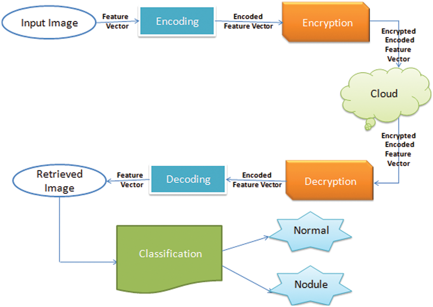
Figure 2: Proposed system diagram

Given its large size, the image (1) congests the network at transmission, (2) requires complex encryption techniques to guarantee privacy, and (3) consumes high encryption time. The proposed technique uses a neural network (an auto-encoder) for fast compression. The reduced-size image is then encrypted with a simple, and fast encryption technique. As the image is not the original one, any encryption technique will suffice to change the image into an unrecognizable one. The integration of the auto-encoder proceeds with an encryption method and is an efficient model for safe image transmission with a low overhead.

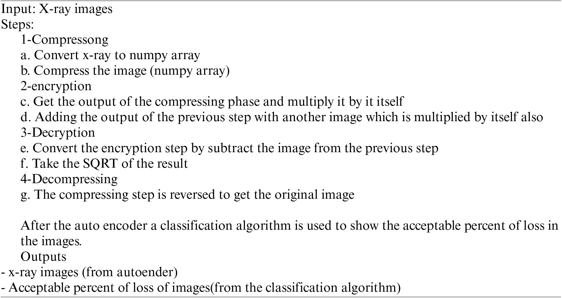
The algorithm steps for the compression and encryption of the image before it is sent over the internet are as follows:

1.    The image is compressed using an auto-encoder.

2.    A specific equation is applied to the output of the auto-encoder to encrypt the image.

The reverse of the previous step is then performed as follows:

1.    Calculate the square root of the vector and then subtract the added image (vector) from it.

2.    Decode to obtain the transferred image with some allowed loss.

To evaluate the loss and ensure that the content is not distorted, the reconstructed images are fed into a classifier to be recognized for medical diagnosis, as shown in Fig. 2.

Fig. 3 shows the modified auto-encoder, which has a 200 × 200 pixel in image size as the input to the encoder. The resulting feature vector from the encoder represents the input to the encryption block and yields the output as an encrypted feature vector. The transmitted vector is decrypted and then decoded to retrieve the original image. The hyperparameters of the auto-encoder affect the output image. Thus, a CNN with different numbers of layers (but the main model has three layers) was utilized to test the changes in the hyperparameters in the AE and the effect of the results on the classification stage. Our main auto-encoder consisted of three layers (three convolutions and two max pooling) as an encoder and another three for the decoder, as follows:

•   Layer 1: The first layer in the encoder was the input layer, consisting of 32 nodes, which had a 200 × 200 input image, with a (3, 3) filter. Each image had the same padding. The pooling layer for the first layer was a MaxPooling2D layer with a (2, 2) pool size.

•   Layer 2: The second layer had 64 nodes, used the ReLU activation function with a (3, 3) filter, and utilized the same padding for the image. Another MaxPooling2D layer with a (2, 2) pool size as the pooling layer for the second one.

•   Layer 3: The third layer is a convolution 2D (Conv2D) layer with the same criteria as the convolution layers but with 128 nodes.

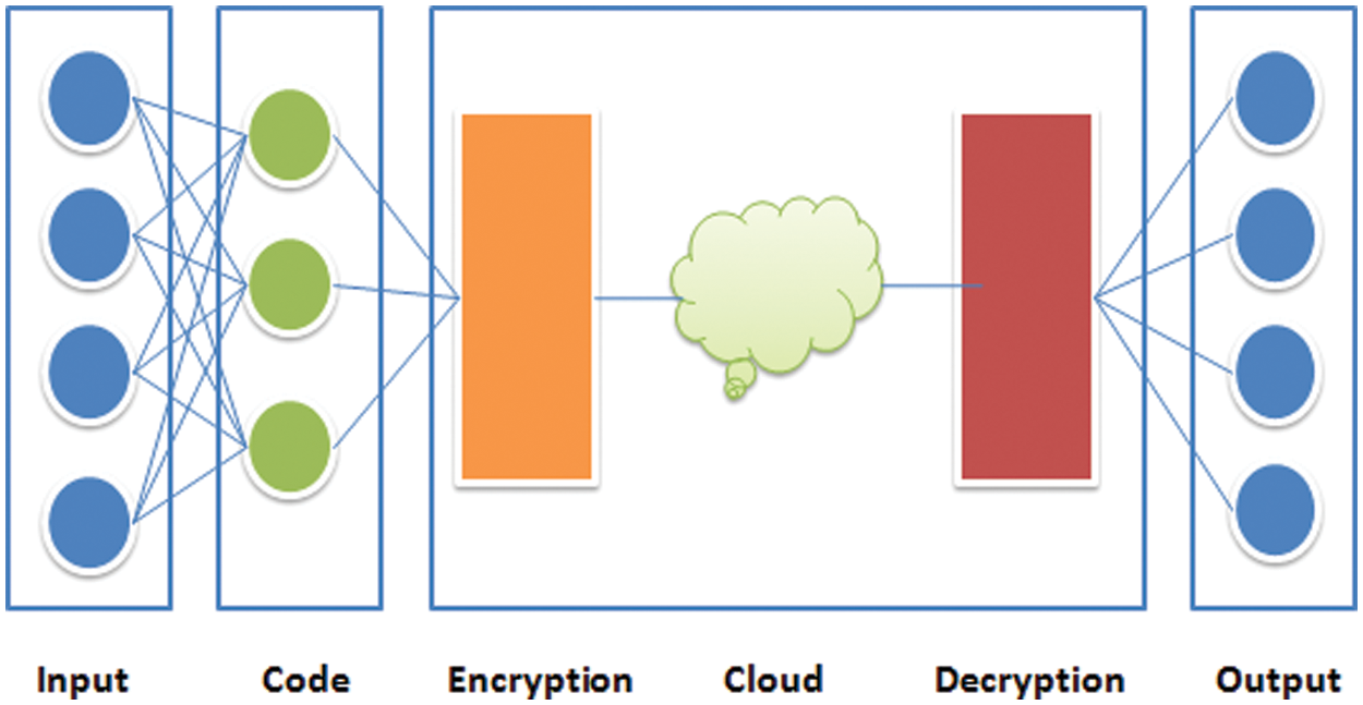
Figure 3: Modified auto-encoder

The decoder also consisted of three layers that were in reverse order to those of the encoder.

•   The first layer was the input layer of the decoder. The input of this layer was the feature vector that resulted from the encoder.

•   The second layer was a Conv2D layer with the same criteria as in the convolution layer in the encoder but with 128 nodes. Then, there was an UpSampling2D layer with a (2, 2) filter.

•   The third layer was the convolution layer but with 64 nodes, followed by an UpSampling2D layer. The final layer was the convolution layer, with 32 nodes and a sigmoid function.

The difference between the auto-encoder discussed in Fig. 1 and the proposed model is that there is an encryption-decryption phase between the encoding and decoding phases.

The encryption function between the encoder and the decoder takes the resulting feature vector from the encoder as an input. At this stage, another image is added to the original image to hide it, and then the square is calculated of the resulting feature vector, as shown in Fig. 4.

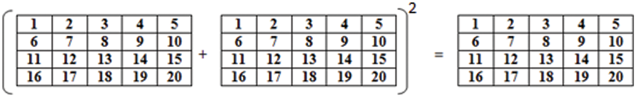
Figure 4: The equation used for encryption

The equation used for encryption is shown above. In the decryption step, the encrypted image (feature vector) is used and subtracted from the added image (vector). Then, the square root is calculated for the resultant vector. The resulting vector from the decryption step is the input vector to the decoder, which is used to retrieve the original image (Fig. 5).

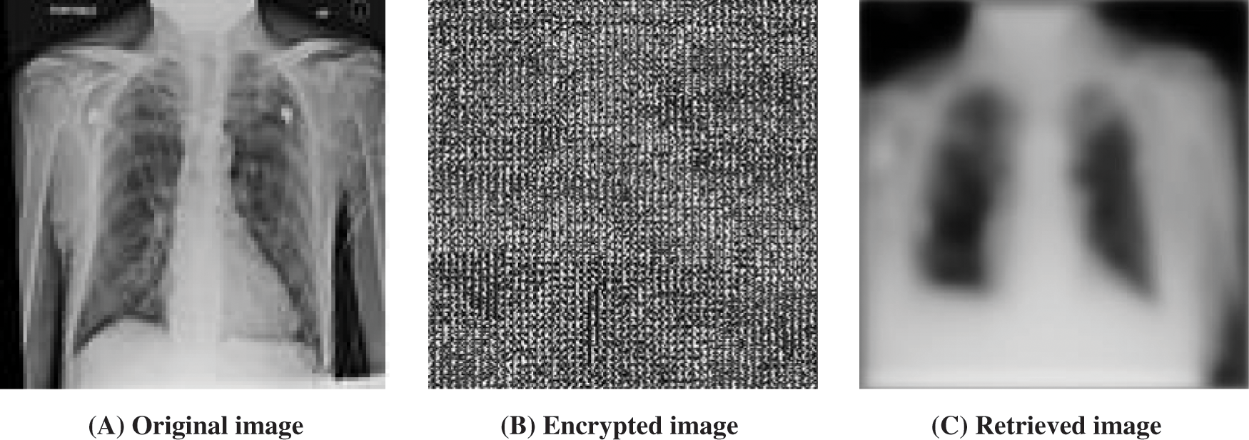
Figure 5: (A) shows the original image; (B) is the encrypted image after applying encoding and encryption; (C) is the retrieved equation after applying decryption and decoding

Our algorithm for the X-ray image can be summarized as follows:

1.    The X-ray image is decoded using a CNN auto-encoder.

2.    The encoder’s output, which is an encoded vector, is then encrypted by adding it to another image and using the power function on the feature vector.

3.    In the decryption step, the image (vector) is subtracted from the resulting vector, and then the power function is reversed using the square root function.

4.    The decrypted image is then decoded to retrieve the original image.

5  Experimental Results and Discussion

5.1 Dataset

Our dataset was extracted from the clinical PACS database within the National Institutes of Physical Fitness Clinical Center and consists of 60% of all informed chest X-rays in the hospital [21]. Therefore, this dataset is considered to be highly associated with the actual human patient population distributions and realistic. This dataset contains several images of healthy and non-healthy volunteers. We used 5000 images to train the auto-encoder and another 5000 to predict and train the classifier. As shown in Fig. 6, the number of negative cases was 5800 and the number of positive cases was 3200.

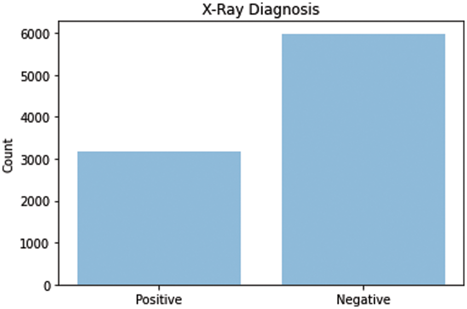
Figure 6: Positive and negative X-rays

5.2 Experiment

Some different hyperparameters were examined, such as the loss function, optimizers, number of layers, number of nodes, number of epochs, and activation function on the auto-encoder. Different measures of metrics were calculated. The source code can be found at the following link [22].

Fig. 7 shows the different metrics used to evaluate the auto-encoder, such as the mean square error (MSE) and the mean absolute error (MAE). The model with the combination of the loss function (mean square logarithmic error), optimizer (ADAM), activation function (ReLU), and 3-layer auto-encoder provided the best results, with a minimum MSE and MAE.

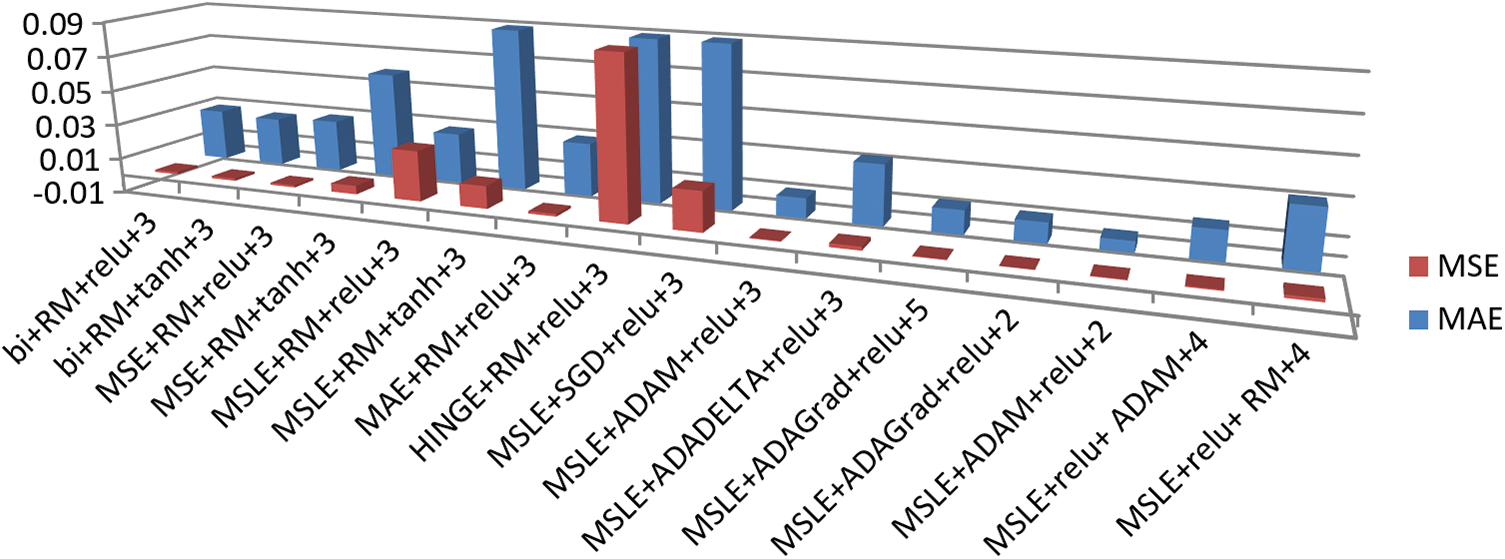
Figure 7: Mean square error (MSE) and mean absolute error (MEA) for the different hyperparameter combinations in the auto-encoder

Fig. 8 shows the loss function of the auto-encoder with different hyperparameters. This loss function occurs at 10, 25, and 50 epochs. As shown in the graph, more than one combination results in a minimum loss, as the last five combinations from the right. Fig. 8 shows some ups and downs, which indicates that the three combinations with the ups have the biggest values in the loss function with the least accurate model.

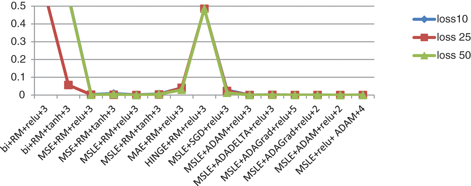
Figure 8: The loss function in different numbers of epochs (10, 25, 50) for the different hyperparameter combinations in the auto-encoder

After retrieving the image, we need to validate its resolution, specifically the use of different hyperparameters on the auto-encoder. Thus, the image was diagnosed using a classifier. Fig. 9 shows the different measures, such as recall, precision, F1, and area under the curve (AUC), of the classification algorithm for the use of different hyperparameters of the auto-encoder. The diagnostic classifier is another CNN classifier used to test the amount of image distortion caused by the application of different hyperparameters on the transmitted image. This was to demonstrate that the distortion was minimal, and thus acceptable, and that the image was diagnosed as required through a classification step.

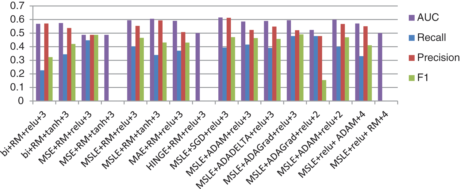
Figure 9: Recall, precision, F1 measure, and AUC for the classifier on the retrieved images after applying different hyperparameter combinations in the auto-encoder

After retrieving images from the auto encoder, a classification algorithm is utilized to show the acceptable amount of damage in the original image. Fig. 10 shows the training accuracy and the testing accuracy of the images resulting from changing auto encoder parameters. The best result is gotten from the third hyperpparameter combination; the last combination gives the worst. The details of the results of the effects of the different hyperparameters on the classification are as follows:

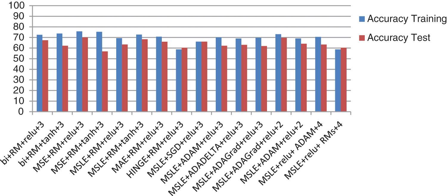
Figure 10: The training accuracy and test accuracy of the classifier on the retrieved images after applying different hyperparameter combinations to the auto-encoder

In Case 1, the best results are achieved for the auto-encoder with RMSprop as an optimizer, three layers for the encoder, and another reverse for the decoder, with ReLU as the activation function. Each epoch consumed takes 15 s to run. Table 1 shows the loss parameters of the training and validation iterations.

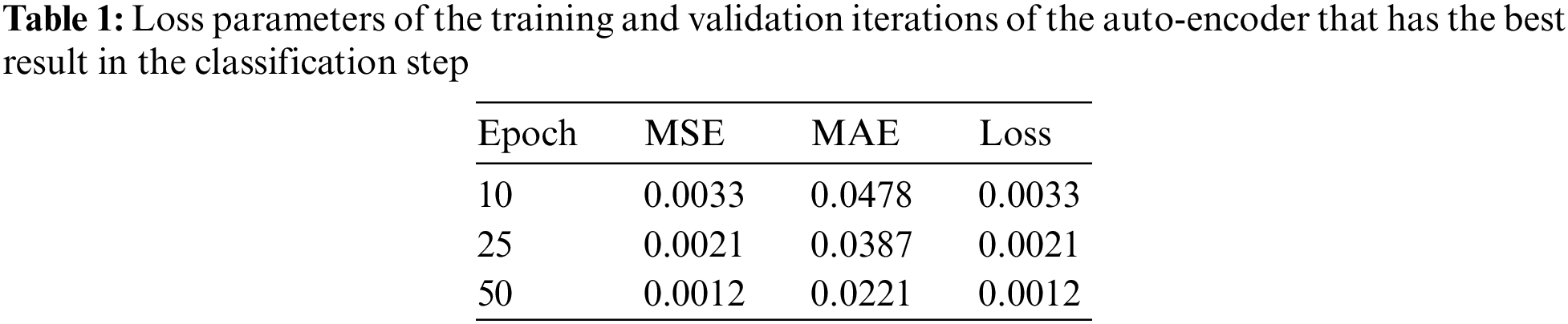
Table 1 shows the MSE, the MAE and the loss function with 10 epochs, 25 epochs and 50 epochs. This table shows that the increase in the epochs decreases the three evaluation functions. The training and validation sets decreased as the epochs increased. The parameters for the auto-encoder provided the best results in the classification model. Fig. 11 shows the training and testing loss function curves of the auto-encoder hyperparameter results for Case 1.

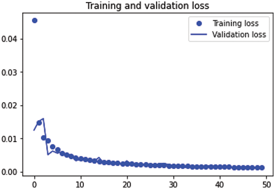
Figure 11: The training and testing loss functions

Table 2 shows the values of the following measures: training accuracy, test accuracy, precision, recall, F1-score, and AUC of the classifier. Table 2 shows the training accuracy, and the test accuracy, recall, precision, F1-score and AUC of the model in the first case. Case 1 shows the best evaluation matrices more than the other two cases.

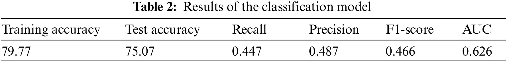
Fig. 12 shows the confusion matrix of the classification stage. The matrix presents the performance of the classification model and the relationship between the predicted and actual values. The first cell shows a false-negative result. The second cell shows the true-negative results, and the third one shows the percentage of the true results according to the whole result (which is 41e+03). In the second row, the first cell is the false positive. The second cell is the true positive. It also shows the iterations in the classification step vs. the loss function (the loss function increases and decreases according to the number of epochs until it remains slightly fixed).

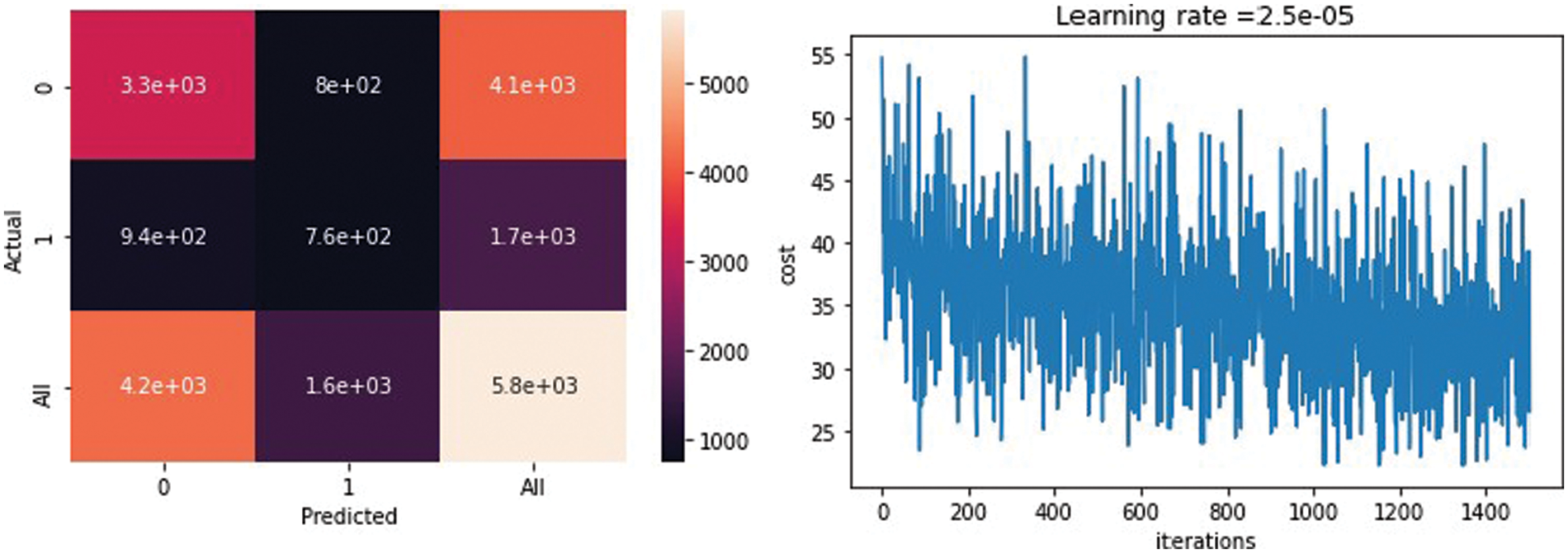
Figure 12: Left: The confusion matrix, and right: The iterations in the classification step

In Case 2, the results of the auto-encoder are not good as in Case 1. This case used mean square logarithmic error as the loss function, ADAGrad as an optimizer, two layers for the encoder, with another set of layers reversed for the decoder and ReLU as the activation function. Each epoch consumed 10 s.

Table 3 presents the auto-encoder evaluation parameters like MSE, MAE, and loss function. It shows that the evaluation function is not so good. The evaluation matrices decrease with the increase of the epoch’s numbers.

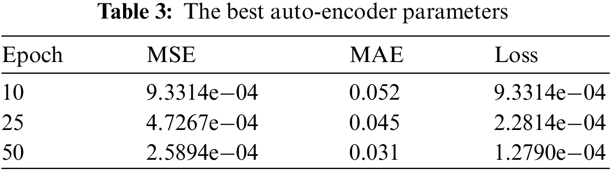
Fig. 13 shows the training and testing loss functions in the auto-encoder hyperparameter results in Case 2. It shows the decrease of the loss function during the increase in the epoch numbers.

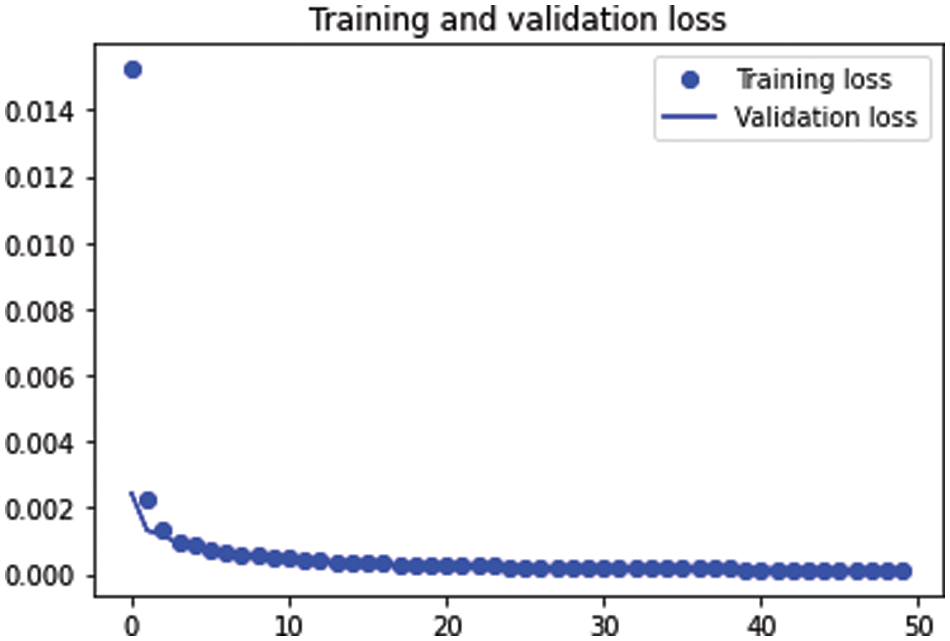
Figure 13: The training and testing loss function

Table 4 shows the different parameters of the classification, such as the training accuracy, test accuracy, precision, recall, F1-score, and AUC (which were not the best values). In Case 2, the results of the auto-encoder reflected on the evaluation of the classification algorithm.

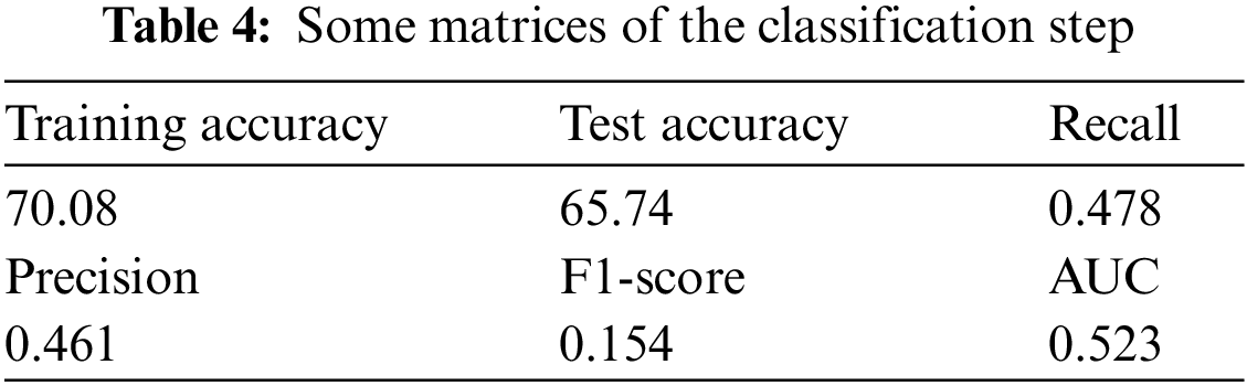
Fig. 14 shows the confusion matrix of the classification stage. The matrix presents the performance of the classification model and the relationship between the predicted and actual values. The first cell shows a false-negative result. The second cell shows the true-negative results, and the third one shows the percentage of the true results according to the whole result (which was 17e+03). In the second row, the first cell is a false positive. The second cell is the true positive. The figure also shows the iterations in the classification step vs. the loss function (the loss function increases and decreases according to the number of epochs until it remains slightly fixed).

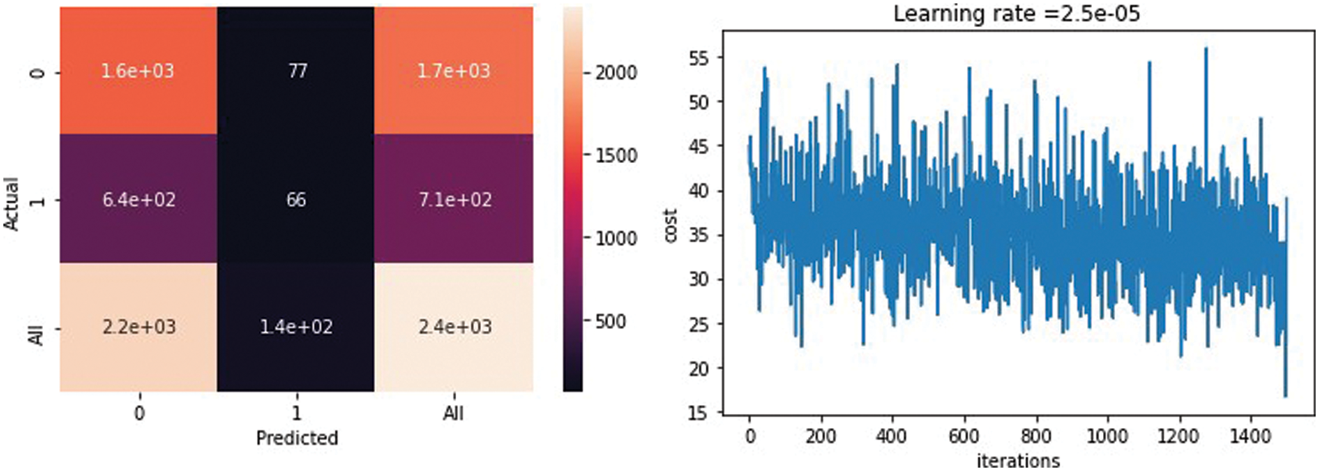
Figure 14: Confusion matrix and iterations in the classification step

Case 3 had the worst classification results after applying the auto-encoder that used hinge as the loss function, RMSprop as an optimizer, three layers for the encoder, with another set of layers reversed for the decoder, and ReLU as the activation function. The total run time for each epoch consumed was 14 s.

Table 5 shows the loss parameter of the training and validation iterations. All matrices remained the same with increasing epochs, even in the validation set, which indicates that there was no learning from the model side, even with increasing epoch numbers. This table shows the worst evaluation matrices in the auto-encoder algorithm.

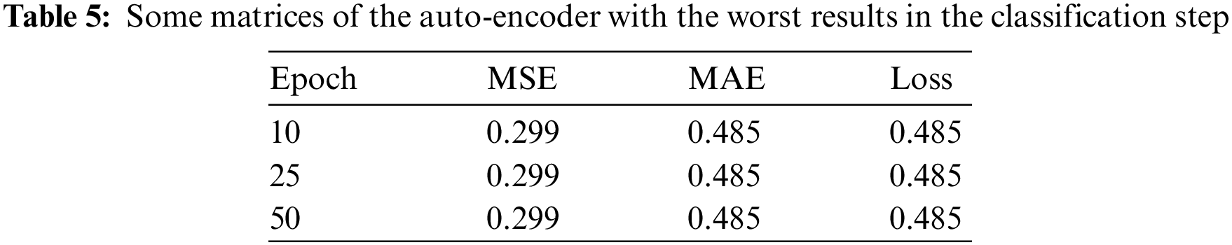
Fig. 15 shows the training and testing loss function in the auto-encoder hyperparameter results in Case 3. The training and testing loss function remain the same which means there is no earning during the training or the validation phases.

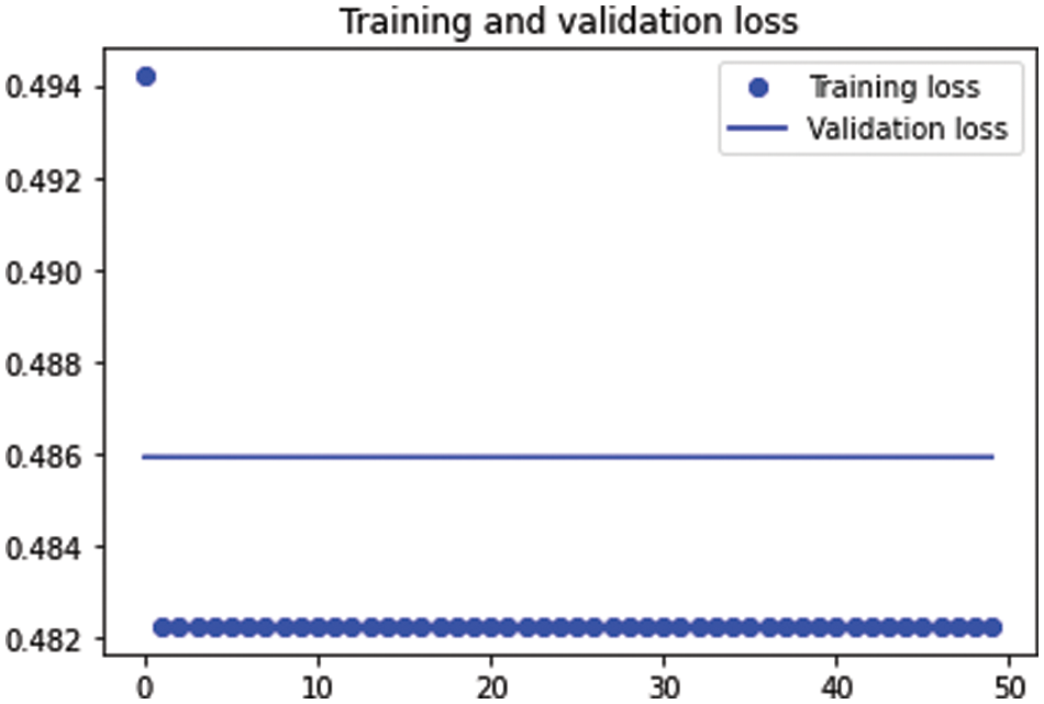
Figure 15: The training and testing loss function

Table 6 shows the different parameters of the classification, such as the training accuracy, test accuracy, precision, recall, F1-score, and AUC (which were the worst values). These matrices ensure the results of the autoenceder, which gives the worst case in all cases with zero recall, precision, and F1-score.

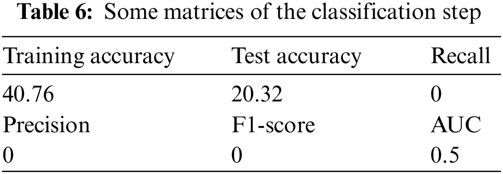
Fig. 16 shows the confusion matrix of the classification stage. The results of the predicted vs. the actual were not good; the expected results were not obtained. The figure also shows the iterations in the classification step vs. the loss function (the loss function did not yield any good results). The model of that combination of hyperparameters gives the worst retrieved image and that reflected on the classification algorithm results which are precision = 0, F1-score = 0, and recall = 0. The blank graph shows the classification model failure.

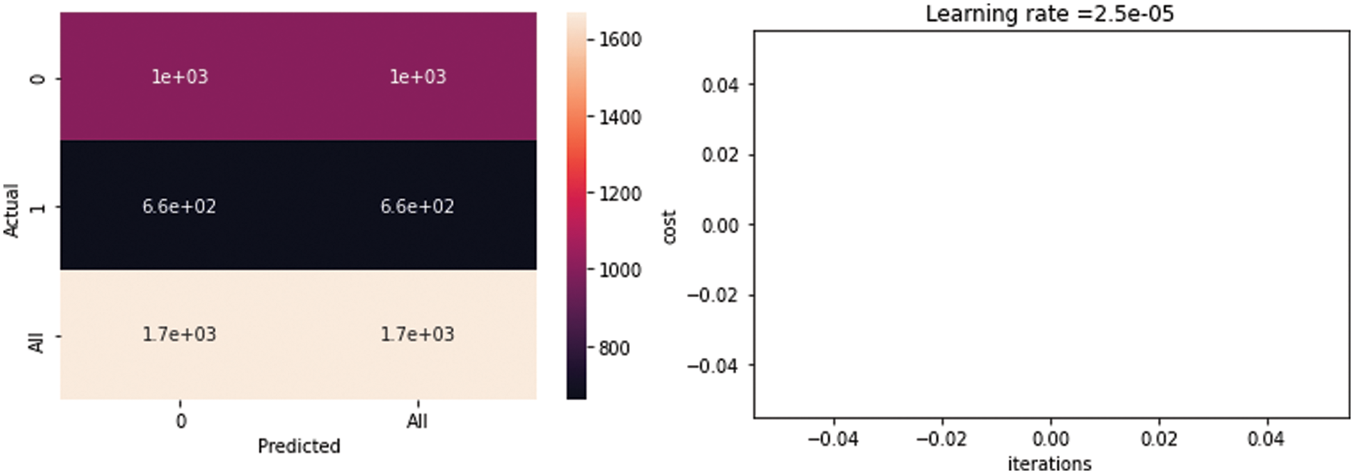
Figure 16: Confusion matrix and iterations in the classification step

Fig. 17 presents the ROC curve of the classification algorithm, reflecting the effects of various hyperparameters on the classification results. The combination of the mean square logarithmic error loss function, the ADAGrad optimizer, the ReLU activation function, and two CNNs (MSLE+ADAGrad+ReLU+2 layers) shows the best curve, compared to combining the mean square logarithmic error loss function. A combination of the mean square logarithmic error loss function, the ADAM optimizer, the ReLU activation function, and two CNN (MSLE+ADAM+ReLU+2 layers), or the mean square logarithmic error loss function, the ADAM optimizer, the ReLU activation function, and five CNN (MSLE+ADAM+ReLU+3 layers).

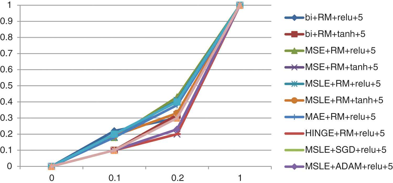
Figure 17: The ROC curve of the classifier on the retrieved images obtained by applying different hyperparameters in the auto-encoder

6  Conclusion

In this study, we provided some deep knowledge, describing various state-of-the-art auto-encoder architectures and showing the usefulness of compressing and encrypting medical images during transmission across an IoT system. We explained the auto-encoder and how different parameters can change its performance and the matrices of the classification algorithm. Based on our findings, we concluded that changing the algorithm hyperparameters may affect the algorithm matrices and the number of epochs. Our findings show that increasing the number of epochs decreases the loss function, while increasing the number of layers does not increase the evaluation matrices. Further, the optimizer ADAM and ADAGrad yielded the best results when applying the auto-encoder with the ReLU activation function and loss function mean square logarithmic error. Early stopping can also give good results. This paper presents a novel auto-encoder model for compressing and encrypting medical images during internet transfer. This model is very important because of the hacking processing over the internet, especially when transferring medical images. Compressing the images is important to speed up the process of transferring images. In future work, some other auto-encoder hyparameter permutations can be utilized. Another classification algorithm with a lot of critical structure can be used to get better results.

Acknowledgement: The authors extend their appreciation to The Institute for Research and Consulting Studies at King Khalid University through Corona Research (Fast Track).

Funding Statement: The funding was provided by the Institute for Research and Consulting Studies at King Khalid University through Corona Research (Fast Track) [Grant No. 3-103S-2020].

Conflicts of Interest: The authors declare that they have no conflicts of interest to report regarding the present study.

References

 1.  Hasan, M., Islam, M. M., Zarif, M. I. I., Hashem, M. M. A. (2019). Attack and anomaly detection in IoT sensors in IoT sites using machine learning approaches. Internet of Things, 7(20), 100059. DOI 10.1016/j.iot.2019.100059. [Google Scholar] [CrossRef]

 2.  Luo, T., Nagarajan, S. G. (2018). Distributed anomaly detection using auto-encoder neural networks in WSN for IoT. IEEE International Conference on Communications (ICC), pp. 1–6. [Google Scholar]

 3.  Chen, L., Guan, Q., Feng, B., Yue, H., Wang, J. et al. (2019). A multi-convolutional auto-encoder approach to multivariate geochemical anomaly recognition. Minerals, 9(5), 270. DOI 10.3390/min9050270. [Google Scholar] [CrossRef]

 4.  Díaz, M., Martín, C., Rubio, B. (2016). State-of-the-art, challenges, and open issues in the integration of Internet of Things and cloud computing. Journal of Network and Computer Applications, 67(7), 99–117. DOI 10.1016/j.jnca.2016.01.010. [Google Scholar] [CrossRef]

 5.  Bhat, S., Bhat, O., Gokhale, P. (2018). Applications of IoT and IoT: Vision 2020. International Advanced Research Journal in Science, Engineering and Technology, 5(1), 41–44. DOI 10.17148/IARJSET.2018.516. [Google Scholar] [CrossRef]

 6.  Maniyath, S. R., Thanikaiselvan, V. (2020). An efficient image encryption using deep neural network and chaotic map. Microprocessors and Microsystems, 77(12), 103134. DOI 10.1016/j.micpro.2020.103134. [Google Scholar] [CrossRef]

 7.  Ameen, S. Y., Othman, K. M., Al-Jammas, M. H. (2012). Neural network-based stream image encryption. Caledonian Journal of Computer, 8, 4–8. [Google Scholar]

 8.  Chauhan, M., Prajapati, R. (2014). Image encryption using chaotic based artificial neural network. International Journal of Scientific & Engineering Research, 5(6). [Google Scholar]

 9.  Elgeldawi, E., Sayed, A., Galal, A. R., Zaki, A. M. (2021). Hyperparameter tuning for machine learning algorithms used for arabic sentiment analysis. Informatics, 8(4), 79. DOI 10.3390/informatics8040079. [Google Scholar] [CrossRef]

10. Baldi, P. (2012). Auto-encoders, unsupervised learning, and deep architectures. Proceedings of ICML Workshop on Unsupervised and Transfer Learning. pp. 37–49. California, USA. [Google Scholar]

11. Wu, J., Chen, X. Y., Zhang, H., Xiong, L. D., Lei, H. et al. (2019). Hyperparameter optimization for machine learning models based on Bayesian optimization. Journal of Electronic Science and Technology, 17(1),26–40. DOI 10.11989/JEST.1674-862X.80904120. [Google Scholar] [CrossRef]

12. Kotsiantis, S. B., Zaharakis, I. D., Pintelas, P. E. (2006). Machine learning: A review of classification and combining techniques. Artificial Intelligence Review, 26(3), 159–190. DOI 10.1007/s10462-007-9052-3. [Google Scholar] [CrossRef]

13. Yang, X., Zhang, X., Ye, Y., Lau, R. Y., Lu, S. et al. (2020). Synergistic 2D/3D convolutional neural network for hyperspectral image classification. Remote Sensing, 12(12), 2033. DOI 10.3390/rs12122033. [Google Scholar] [CrossRef]

14. Hu, F., Wang, J., Xu, X., Pu, C., Peng, T. (2017). Batch image encryption using generated deep features based on stacked autoencoder network. Mathematical Problems in Engineering, 2017(1), 1–12. DOI 10.1155/2017/3675459. [Google Scholar] [CrossRef]

15. Thanikaiselvan, V., Mantripragada, N., Singh, A. P., Bhasin, N. (2019). Encrypting multiple images using stacked autoencoders. 2019 International Conference on Vision Towards Emerging Trends in Communication and Networking (ViTECoN), pp. 1–6. Vellore, India, IEEE. [Google Scholar]

16. Sushmit, A. S., Zaman, S. U., Humayun, A. I., Hasan, T., Bhuiyan, M. I. H. et al. (2019). X-ray image compression using convolutional recurrent neural networks. IEEE EMBS International Conference on Biomedical & Health Informatics (BHI), pp. 1–4. Chicago, IL, USA, IEEE. [Google Scholar]

17. Akyazi, P., Ebrahimi, T. (2019). Learning-based image compression using convolutional autoencoder and wavelet decomposition. IEEE Conference on Computer Vision and Pattern Recognition Workshops, London, UK. [Google Scholar]

18. Vu, L., Cao, V. L., Nguyen, Q. U., Nguyen, D. N., Hoang D. T. et al. (2020). Learning latent representation for IoT anomaly detection. IEEE Transactions on Cybernetics. DOI 10.1109/TCYB.2020.3013416. [Google Scholar] [CrossRef]

19. Ameen Suhail, K. M., Sankar, S. (2020). Image compression and encryption combining autoencoder and chaotic logistic map. Iranian Journal of Science and Technology, Transactions A: Science, 44(4), 1091–1100. DOI 10.1007/s40995-020-00905-4. [Google Scholar] [CrossRef]

20. Mohammadi, M., Al-Fuqaha, A., Sorour, S., Guizani, M. (2018). Deep learning for IoT big data and streaming analytics: A survey. IEEE Communications Surveys & Tutorials, 20(4), 2923–2960. DOI 10.1109/COMST.2018.2844341. [Google Scholar] [CrossRef]

21. Mooney, P. (2007). Data set. https://www.kaggle.com/paultimothymooney/chest-xray-pneumonia. [Google Scholar]

22. https://github.com/maiemahmoud/auto-encoder. 2020. [Google Scholar]