1 Introduction
Laminated materials are very often required in many engineering applications. In particular, an increasing need for structures with complex geometric shapes characterized by smart non-conventional fabrics is much more evident [1–4]. In this way, an optimization of the material properties can be obtained from the model, since the lamination scheme can be selected according to the structural needs, especially when the geometry cannot be varied due to architectural and functional requirements [5,6]. On the other hand, the introduction of curvature provides an optimization of the stress distribution. Nevertheless, classical models can lead to erroneous predictions due to an unusual structural behaviour coming from the absence of material and geometric symmetry planes [7–10]. In order to prevent the invalidation of the design process and exposing the final product to some safety risks, new simple but accurate methodologies should be developed. Furthermore, a proper mathematical modelling of complex appliances, embedding all the curvature effects and constitutive couplings, can be very cumbersome in its conception as well as computationally demanding, due to the huge number of variables occurring in the structural problem [11,12]. Three-dimensional elasticity solutions are the most accurate approaches for the correct prediction of a structural response [13–15]. However, in the case of anisotropic materials and complicated structural shapes, a closed-form solution can not be easily found. Therefore, a large numerical system should be developed with a significative number of Degrees of Freedom (DOFs). This is likely to come across several numerical issues like the computational stability. For this reason, simplified two-dimensional formulations have been developed throughout literature, so that the solution is found with a lower computational effort [16–20]. In particular, two main approaches can be traced, namely the Equivalent Single Layer (ESL) and Layer-Wise (LW) formulations [21–24]. According to ESL, the three-dimensional doubly-curved solid is reduced to a surface located in its middle thickness. In this way, a 2-manifold is derived with its geometric parameters describing the shape of the actual structure [25,26]. Moreover, the field variable, as well as the primary and secondary ones, are reduced to the surface at issue. A key aspect of this approach is the homogenization of the stacking sequence so that a set of equivalent properties can be computed. In contrast, the two-dimensional LW implementations account for a displacement field expansion within each lamina, thus providing an accurate local description of all the mechanical quantities. Furthermore, compatibility conditions are developed between two adjacent laminae so that the consistency of the whole model is assessed [27,28]. Within the LW approach, the accuracy of the solution may be increased if the order of the adopted interpolating polynomials gets higher, or equivalently if a generic lamina is divided in some virtual sub-layers following a local-global strategy, thus leading to sub-laminate formulations [29–36]. As far as the displacement field assumption is concerned, classical approaches provide a linear through-the-thickness assumption of the unknown in-plane field variables, whereas a rigid behaviour is assumed in the out-of-plane directions. In this way, no stretching effects can be predicted, as well as the softcore behaviour of the lamination scheme [37]. In addition, a smooth displacement field assumption does not fit the actual interlaminar deformation during the deflection of the structure. For this reason, a higher order axiomatic expression for the out-of-plane variable is crucial in both LW and ESL approaches, even though the latters should embed in themselves with the well-known zig-zag function in order to obtain accurate results [38–43]. A milestone for the assessment of the kinematic field variable is its unified description [44,45], which incorporates both higher order theories and classical approaches like the First Order Shear Deformation Theory (FSDT) and the Third Order Shear Deformation Theory (TSDT), outlined in references [46,47]. Since it allows the introduction of a generalized set of thickness functions in both in-plane and out-of-plane directions, polynomials, non-polynomials and trigonometric functions can be employed to this purpose [48–50], depending on the material properties and relative thickness of the laminae embedded in the structure. Moreover, it is possible to develop an advanced set of axiomatic thickness functions, whose expressions is obtained from the mechanical shear properties of the lamination scheme, leading to the so-called refined zig-zag theories [51–53].
The fundamental governing equations have been analytically solved only for simple geometries and lamination schemes, such as frames, plates, cylinders and spherical panel. On the other hand, only cross-ply orthotropic laminates can be adopted, otherwise no mathematical procedures are available at the moment for the solutions of such differential sets of equations. For this reason, in references [54,55] the ESL structural problem for structures with single and double curvatures accounting for a generally anisotropic lamination scheme is numerically developed by means of the Generalized Differential Quadrature (GDQ) method. We recall that such methodology discretizes directly the derivatives of a given function, thus allowing to solve the problem directly in the strong form, as it has been shown in references [56–60]. Belonging to the class of spectral collocation methods, it embeds a series of numerical techniques like the gaussian quadrature and the classical differential quadrature [61,62], accounting for a rectangular computational grid. The accuracy of the method comes from the proper selection of a set of discrete points from the physical domain, as well as the computation of the quadrature coefficients. In references [63,64] its accuracy has been compared to other numerical techniques. Moreover, it has been shown that it is a very reliable procedure for the analysis of lattice three-dimensional cells [65–67], as well as Functionally Graded Materials (FGMs) employing a reduced computational cost [68–71]. Moving from the above discussed GDQ procedure, the Generalized Integral Quadrature (GIQ) method turns out to be an effective strategy for the numerical implementation of integrals with a domain collocation strategy. In references [72,73], the interested reader can find an extended treatise on the topic.
In classical variational approaches like the well-known Finite Element Method (FEM), an axiomatic set of shape functions are provided, leading to a weak form of the governing equations [74–76]. However, this methodology induces some drawbacks in the solution due to the discrepancy between the geometry and the adopted interpolating function. As a matter of fact, this problem can be overcome if a domain is discretized with a fine mesh, which in turn increases the computational cost. In contrast, the Iso-Geometric Approach (IGA) adopts the actual geometry of the structure employed in the Computer Aided Design (CAD) procedure itself for the assessment of the unknown field variable of the governing equations. Starting from the pioneer works reported in reference [77], the IGA methodology has been successfully applied to several structural problems related to arbitrary shapes [78,79]. It has been shown that IGA is a very efficient methodology in the case of structures of arbitrary geometries, especially when a significative domain distortion is required. In particular, the best performances of such methodology are reached when Non-Uniform Rational Basis Spline (NURBS) curves with higher order basis functions are adopted because they show a significative computational stability. In references [80,81], the curves at issue are presented in a comprehensive way, together with an iterative procedure for their computation. Furthermore, in references [82–83], a meshfree Galerkin method is applied for the buckling analysis of shallow shells with single and double curvatures accounting for geometric interpolation functions for the assessment of the unknown field variable. In reference [84], the meshfree approach has been adopted for the finite rotation analysis of structures with different curvatures.
Another topic related to the analysis of shell structures relies on the computation of concentrated loads within the structural problem. In classic domain decomposition procedures like FEM, generalized forces are applied at a specific node of the domain mesh [85,86]. If the load is not applied in a computational point, a set of equivalent forces are derived by means of an interpolating procedure employing the adopted shape functions. The same approach can be found in references [87,88] where the GDQ algorithm has been adopted within each element in which the domain has been divided. As a consequence, a concentrated force pretends to be a boundary condition within the differential model. On the other hand, in the case of a problem developed within a single domain, in references [89–91], an interesting procedure based on GDQ and GIQ methods accounts for a differential-integral implementation on a rectangular plate under a concentrated load, taking into account the main features of the well-known Dirac-Delta function [92]. On the other hand, a concentrated load can be seen as a particular case of a surface pressure acting on a very small area. Nevertheless, the distribution governing parameters should be set according to the actual dimension of the structure object of analysis [93,94].
In the present manuscript, a LW formulation is derived for the static analysis of generally anisotropic shell structures with a double curvature under the action of concentrated loads. The unknown displacement field variable is described, within each layer, employing a generalized approach with different higher order thickness functions. Furthermore, the displacement compatibility conditions between two adjacent layers are fulfilled. The geometry of the shell is described with curvilinear principal coordinates and a mapping procedure is adopted for arbitrarily-shaped structures. A generally anisotropic elastic behaviour is considered within each lamina. The fundamental set of differential equations is derived following an energy approach, together with the kinematic and static boundary conditions by means of a strong formulation of the structural problem. Then, non-conventional external constraints are enforced within the two-dimensional model. The differential problem is tackled numerically with the GDQ method, accounting for the discretization of the derivatives of a generic order, whereas integrals are solved with the GIQ numerical algorithm. Since the numerical model embeds in itself a smooth variation of derivatives, both surface distributed and concentrated loads are modelled with a comprehensive set of bivariate distributions, whose governing parameters have been carefully calibrated. Furthermore, the Dirac-Delta function is adopted in its classical and generalized GDQ discrete version for the assessment of concentrated loads [95–97]. The main elements of novelty of the proposed method are the efficient numerical implementation of the concentrated load, which is a singularity among surface tractions, directly in the continuum model. Furthermore, the normalization of the distribution with respect to the surface area provides an effective calibration of the shape and position parameters. In the post-processing stage, an effective reconstruction of physical quantities throughout the entire shell thickness is assessed based on the three-dimensional static balance equations for a laminated anisotropic solid applied to each layer of the stacking sequence. A significative number of numerical investigations have been attached to the manuscript. The accuracy of the numerical predictions has been checked with respect to refined three-dimensional Finite Element models developed with a commercial package, showing a very good agreement between different approaches. Moreover, the inconsistency of higher order ESL formulations has been outlined for very thick structures characterized by very complex lamination schemes with a huge number of laminae with various material syngonies. Then, the solution has been checked for both single and double curvatures. The proposed higher order LW formulation has been added to the Differential Quadrature for Mechanics of Anisotropic Shells, Plates, Arches and Beams (DiQuMASPAB) project [98], a free research software which provides the static and the dynamic response of doubly-curved shell structures with various ESL and LW theories.
2 Doubly-Curved Shell Geometry
A doubly-curved shell is a three-dimensional solid within the Euclidean space (Fig. 1). For this reason, if e1,e2,e3 are the unit vectors of a global coordinate system, the position vector R(α1,α2,α3) of an arbitrary point of the structure can be described in terms of the following relation [21]:

Figure 1: Geometric assessment of a doubly-curved shell according to a LW approach. Representation of a generic thickness function of different orders defined in each k-th layer of the stacking sequence for k=1,…,l, being l the total number of laminae occurring in the lamination scheme
R(α1,α2,α3)=f1(α1,α2,α3)e1+f2(α1,α2,α3)e2+f3(α1,α2,α3)e3(1)
where f1,f2,f3 are functions of the variables α1,α2,α3. It should be said that Eq. (1) assumes a physical meaning if the variations αi0≤αi≤αi1 for i=1,2,3 are declared, being αi0,αi1 the extremes of the variation intervals. If a laminated structure composed by l laminae is considered, the overall thickness of the structure h can be computed as the sum of the widths hk of each layer, with k=1,…,l:
h=∑k=1lhk(2)
As a matter of fact, the association α3=ζ is performed so that the axis at issue is oriented alongside the thickness direction of the shell. Moreover, a reference surface r(α1,α2) is assessed, located in the middle thickness of the structure, whose parametric directions α1,α2 are defined from the principal geometric features of the shell. Referring to a generic k-th layer of a laminated structure, a unit vector set O′α1(k)α2(k)ζ(k) is introduced for k=1,…,l. On the other hand, if hk assumes a constant value throughout the entire structure, α1(k)α2(k) can be obtained from an affine transformation alongside ζ direction of α1,α2 in-plane coordinates of the shell reference surface, thus setting αi(k)=αi for i=1,2. As a consequence, a key relation for the LW geometric and mechanic computation is introduced [24], defining the differential variation of local and global thickness coordinates ζ(k) and ζ:
dζ(k)=dζ(3)
In this way, a reference surface r(k)(α1,α2) is defined in the middle thickness of each k-th layer of the stacking sequence starting from the global geometric quantity r(α1,α2) referred to the global curvilinear coordinate O′α1α2ζ according to the following expression [21], as shown in Fig. 1.
r(k)(α1,α2)=r(α1,α2)+ζk+1+ζk2n(α1,α2)(4)
where ζk,ζk+1 denote the extreme locations of the k-th layer along the shell thickness direction, whereas n(α1,α2) accounts for the normal unit vector of the reference surface r(α1,α2), defined as follows:
n(α1,α2)=r,1×r,2|r,1×r,2|(5)
where r,i=∂r/∂αi denotes the partial derivative of the shell reference surface with respect to the already introduced principal direction αi for i=1,2 [21]. Starting from Eq. (4), the thickness curvature parameter Hi(k)(α1,α2) referred to the αi=α1,α2 principal direction is computed:
Hi(k)=1+ζ(k)Ri(k)i=1,2(6)
Furthermore, the Lamé parameters Ai(k)(α1,α2) and the principal curvature radii Ri(k)(α1,α2) of the reference surface of the k-th layer can be computed as:
Ai(k)(α1,α2)=r,i(k)⋅r,i(k)=Ai(1+ζk+1+ζk2Ri)Ri(k)(α1,α2)=−r,i(k)⋅r,i(k)r,ii(k)⋅n=Ri+ζk+1+ζk2fori=1,2(7)
where n is the normal unit vector defined in Eq. (5), whereas r,i(k)=∂r(k)/∂αi and r,ii(k)=∂2r(k)/∂αi2 account for the first and the second order derivative of Eq. (4) with respect to αi=α1,α2, respectively. In addition, Ai=Ai(α1,α2) and Ri=Ri(α1,α2) for i=1,2 are referred to the surface r(α1,α2) located in the middle thickness of the entire laminated structure. From the main outcomes of the differential geometry, such quantities are calculated according to the following expressions, setting r,ii=∂2r/∂αi2 [21]:
Ai(α1,α2)=r,i⋅r,i,Ri(α1,α2)=−r,i⋅r,ir,ii⋅nfori=1,2(8)
Having in mind all these premises, the three-dimensional position vector R(k)(α1,α2,ζ) of a generic point belonging to the k-th layer can be referred to r(α1,α2) as follows (Fig. 1):
R(k)(α1,α2,ζ)=r(α1,α2)+(ζk+1+ζk2+hk2zk)n(α1,α2)(9)
being zk=2ζ(k)/hk a dimensionless thickness coordinate belonging to the interval [−1,1]. It is useful to compute the first order derivative of zk with respect to the local thickness coordinate ζ(k), so that:
∂zk∂ζ(k)=2ζk+1−ζk=2hk(10)
2.1 Arbitrarily-Shaped Shells
When the parametrization of the reference surface does not account for a curvilinear set of principal coordinates, the two-dimensional physical domain is distorted so that a rectangular dimensionless parent element is obtained, described in terms of the natural coordinates ξ1∈[−1,+1] and ξ2∈[−1,+1], as it has been schematically shown in Fig. 2. If we denote with (α1(i),α2(i)) the location of the i-th corner of the distorted geometry, for i=1,…,4, the blending functions presented in the following can be employed [21]:

Figure 2: Isogeometric mapping of the physical domain employing NURBS curves. Definition of the local reference system along the edges of the distorted shell for the assessment of boundary conditions. Derivation of the rectangular computational domain employing natural coordinates
α1(ξ1,ξ2)=12((1−ξ2)α¯1(1)(ξ1)+(1+ξ1)α¯1(2)(ξ2)+(1+ξ2)α¯1(3)(ξ1)+(1−ξ1)α¯1(4)(ξ2))+ −14((1−ξ1)(1−ξ2)α1(1)+(1+ξ1)(1−ξ2)α1(2)+(1+ξ1)(1+ξ2)α1(3)+(1−ξ1)(1+ξ2)α1(4))(11)
α2(ξ1,ξ2) =12((1−ξ2)α¯2(1)(ξ1)+(1+ξ1)α¯2(2)(ξ2)+(1+ξ2)α¯2(3)(ξ1)+(1−ξ1)α¯2(4)(ξ2))+ −14((1−ξ1)(1−ξ2)α2(1)+(1+ξ1)(1−ξ2)α2(2)+(1+ξ1)(1+ξ2)α2(3)+(1−ξ1)(1+ξ2)α2(4))(12)
In the previous equation, (α¯1(j),α¯2(j)) denotes the description in terms of α1,α2 of the j=1,…,4 edge of the structure. To describe a generic curve C(u) with a≤u≤b alongside the physical domain, a combination of n control points Pi for i=1,…,n is employed, as follows (Fig. 2):
C(u)=∑i=0nRi,p(u)Pi(13)
where Ri,p(u) is a rational B-Spline of p-th order which can be computed from the following expression, being wi a proper weighting coefficient:
Ri,p(u)=Ni,p(u)wi∑i=0nNi,p(u)wi(14)
Setting for simplicity [a,b]=[0,1] and introducing a predefined knot vector U=[a,…,a⏟p+1,up+1,…,um−p−1,b,…,b⏟p+1] a recursive relationship can be adopted to compute the B-Spline basis function Ni,p(u) of p-th order. Starting with p=0, it is [21]:
Ni,0(u)={1ifui≤u<ui+10otherwiseNi,p(u)=u−uiui+p−uiNi,p−1(u)+ui+p+1−uui+p+1−ui+1Ni+1,p−1(u)(15)
When arbitrarily-shaped structures are investigated, the fundamental relations, provided in terms of (α1,α2)∈[α10,α11]×[α20,α21], should be expressed in terms of ξ1,ξ2 coordinates within the interval [−1,1]×[−1,1]. If we denote with J the Jacobian matrix of the coordinate transformation α1=α1(ξ1,ξ2), α2=α2(ξ1,ξ2), it can be stated that:
[∂∂ξ1∂∂ξ2]=[∂α1∂ξ1∂α2∂ξ1∂α1∂ξ2∂α2∂ξ2][∂∂α1∂∂α2]=J[∂∂α1∂∂α2](16)
Accordingly, an inversion of Eq. (16) can be performed if det(J)=ξ1,α1ξ2,α2−ξ1,α2ξ2,α1≠0, leading to the definition of the inverse Jacobian matrix J−1:
[∂∂α1∂∂α2]=J−1[∂∂ξ1∂∂ξ2]=1det(J)[∂α2∂ξ2−∂α2∂ξ1−∂α1∂ξ2∂α1∂ξ1][∂∂ξ1∂∂ξ2](17)
Once Eqs. (11) and (12) have been assessed, it is possible to provide an expression to define the first order partial derivatives with respect to α1,α2 principal coordinates in terms of the natural ones ξ1(α1,α2) and ξ2(α1,α2), starting from the well-known derivation chain rule:
[∂∂α1∂∂α2]=[ξ1,α1ξ2,α1ξ1,α2ξ2,α2][∂∂ξ1∂∂ξ2](18)
being ξi,αj=∂ξi/∂αj for i,j=1,2. From a comparison of Eqs. (17) and (18), it is possible to provide the complete expression of ξi,αj coefficients, leading to [21]:
ξ1,α1=∂ξ1∂α1=1det(J)∂α2∂ξ2,ξ2,α1=∂ξ2∂α1=−1det(J)∂α2∂ξ1,ξ1,α2=∂ξ1∂α2=−1det(J)∂α1∂ξ2,ξ2,α2=∂ξ2∂α2=1det(J)∂α1∂ξ1(19)
Based on Eq. (18), it is possible to express the second order derivatives with respect to the principal coordinate α1,α2 in terms of ξ1,ξ2. One gets:
∂2∂α12=ξ1,α12∂2∂ξ12+ξ2,α12∂2∂ξ22+2ξ1,α1ξ2,α1∂2∂ξ1∂ξ2+ξ1,α1α1∂∂ξ1+ξ2,α1α1∂∂ξ2∂2∂α22=ξ1,α22∂2∂ξ12+ξ2,α22∂2∂ξ22+2ξ1,α2ξ2,α2∂2∂ξ1∂ξ2+ξ1,α2α2∂∂ξ1+ξ2,α2α2∂∂ξ2∂2∂α1∂α2=ξ1,α1ξ1,α2∂2∂ξ12+ξ2,α1ξ2,α2∂2∂ξ22+(ξ1,α1ξ2,α2+ξ1,α2ξ2,α1)∂2∂ξ1∂ξ2+ξ1,α1α2∂∂ξ1+ξ2,α1α2∂∂ξ2(20)
Eq. (20) assesses the dependence of the second order derivatives with respect to α1,α2 in terms of the first and second order derivatives with respect to ξ1,ξ2 natural coordinates. Accordingly, the equation at issue is not bi-linear in the present formulation. In the following, the interested reader can find the complete expression of coefficients introduced in Eq. (20):
ξ1,α1α1=1det(J)2(∂α2∂ξ2∂2α2∂ξ1∂ξ2−(∂α2∂ξ2)2det(J)ξ1det(J)−∂α2∂ξ1∂2α2∂ξ22+∂α2∂ξ1∂α2∂ξ2det(J)ξ2det(J))ξ2,α1α1=1det(J)2(−∂α2∂ξ2∂2α2∂ξ12+∂α2∂ξ2∂α2∂ξ1det(J)ξ1det(J)+∂α2∂ξ1∂2α2∂ξ1∂ξ2−(∂α2∂ξ1)2det(J)ξ2det(J))(21)
ξ1,α2α2=1det(J)2(∂α1∂ξ2∂2α1∂ξ1∂ξ2−(∂α1∂ξ2)2det(J)ξ1det(J)−∂α1∂ξ1∂2α1∂ξ22+∂α1∂ξ1∂α1∂ξ2det(J)ξ2det(J))ξ2,α2α2=1det(J)2(−∂α1∂ξ2∂2α1∂ξ12+∂α1∂ξ2∂α1∂ξ1det(J)ξ1det(J)+∂α1∂ξ1∂2α1∂ξ1∂ξ2−(∂α1∂ξ1)2det(J)ξ2det(J))(22)
ξ1,α1α2=1det(J)2(−∂α2∂ξ2∂2α1∂ξ1∂ξ2+∂α2∂ξ2∂α1∂ξ2det(J)ξ1det(J)+∂α2∂ξ1∂2α1∂ξ22−∂α2∂ξ1∂α1∂ξ2det(J)ξ2det(J))ξ2,α1α2=1det(J)2(−∂α2∂ξ1∂2α1∂ξ1∂ξ2+∂α1∂ξ2∂α1∂ξ1det(J)ξ1det(J)+∂α2∂ξ2∂2α1∂ξ12−∂α2∂ξ1∂α1∂ξ1det(J)ξ2det(J))(23)
The first order derivatives det(J)ξ1,det(J)ξ2 of the determinant det(J) of the Jacobian matrix introduced in Eq. (16) with respect to ξ1 and ξ2, respectively, read as follows:
det(J)ξ1=∂α1∂ξ1∂2α2∂ξ1∂ξ2−∂α2∂ξ1∂2α1∂ξ1∂ξ2+∂α2∂ξ2∂2α1∂ξ12−∂α1∂ξ2∂2α2∂ξ12det(J)ξ2=−∂α1∂ξ2∂2α2∂ξ1∂ξ2+∂α2∂ξ2∂2α1∂ξ1∂ξ2−∂α2∂ξ1∂2α1∂ξ22+∂α1∂ξ1∂2α2∂ξ22(24)
A useful nomenclature is now introduced, so that the edges of the physical domain can be univocally identified. Referring to the dimensionless rectangular parent element described in terms of the natural coordinates ξ1,ξ2, the following definitions [21] are outlined (Fig. 2):
West edge(W)→ξ2=−1→(α1,α2)=(α¯1(1)(ξ1),α¯2(1)(ξ1))South edge(S)→ξ1=1→(α1,α2)=(α¯1(2)(ξ2),α¯2(2)(ξ2))East edge(E)→ξ2=1→(α1,α2)=(α¯1(3)(ξ1),α¯2(3)(ξ1))North edge(N)→ξ1=−1→(α1,α2)=(α¯1(4)(ξ2),α¯2(4)(ξ2))(25)
3 Unified Formulations for Kinematic Relations
In the present section a unified assessment of the kinematic field variable is presented following the LW methodology. Referring to a generic k-th lamina of the laminate, each component U1(k)(α1,α2,ζ(k)) for i=1,…,3 of the three-dimensional displacement field column vector U(k)(α1,α2,ζ(k)) can be expanded up to an arbitrary N-th order, thus introducing for each τ=0,…,N+1 a generic function Fταi(k) for i=1,…,3 dependent from the local thickness coordinate ζ(k) [24]:
[U1(k)U2(k)U3(k)]=∑τ=0N+1[Fτα1(k)000Fτα2(k)000Fτα3(k)][u1(kτ)u2(kτ)u3(kτ)]↔U(k)(α1,α2,ζ(k))=∑τ=0N+1Fτ(k)u(kτ)(26)
where u1(kτ),u2(kτ),u3(kτ) are the generalized displacement field components defined for each τ-th kinematic expansion order lying on the r(k)(α1,α2) reference surface of the k-th lamina. In Fig. 1, one can find a graphic representation of Eq. (26).
Since a laminated doubly-curved shell structure is considered with k=1,…,l, where l is the total number of superimposed laminae, the displacement field variable should fulfil the interlaminar compatibility conditions. To this purpose, an interpolation methodology based on higher order polynomials is followed for the definition of Fταi(k) for τ=0,…,N+1. Accordingly, the dimensionless thickness coordinate zk introduced in Eq. (9) is considered:
Fταi(k)={1−zk2forτ=0Lτ(zk)forτ=1,…,N1+zk2forτ=N+1i=1,2,3(27)
where Lτ(zk) for τ=1,…,N is defined employing various interpolating polynomials. As can be seen, Eq. (27) refers to the three-dimensional displacement distribution throughout the thickness. As a consequence, the interlaminar compatibility conditions are directly satisfied by the axiomatic assumptions of the unknown field variable itself. The first order derivative of the generalized thickness functions introduced in Eq. (27) with respect to ζ(k) can be computed as:
∂Fταi(k)∂ζ(k)={−12∂zk∂ζ(k)forτ=0∂Lτ(zk)∂zk∂zk∂ζ(k)forτ=1,…,N12∂zk∂ζ(k)forτ=N+1(28)
As can be seen, the derivatives ∂zk/∂ζ(k) occurring in Eq. (28) are calculated according to Eq. (10).
If power functions are introduced in Eqs. (27) and (28), the following expressions should be adopted for each τ=1,…,N [24]:
Lτ(zk)=zkτ+1−zkτ−1→∂Lτ(zk)∂zk=(τ+1)zkτ−(τ−1)zkτ−2(29)
On the other hand, a formulation based on higher order Lagrange interpolating polynomials reads as follows:
Lτ(zk)=∏m=0,m≠τN+1(zk−zkm)(zkτ−zkm)→∂Lτ(zk)∂zk=∑r=0,r≠τN+1∏m=0,m≠r,τN+1(zk−zkm)∏m=0,m≠τN+1(zkτ−zkm)(30)
If trigonometric functions are adopted in Eq. (27), Fταi(k)=Lτ(zk) for each τ=1,…,N reads as:
Lτ(zk)=cos(−(−1)ττπ2zk+π4(1−(−1)τ+1))→∂Lτ(zk)∂zk=(−1)ττπ2sin(−(−1)ττπ2zk+π4(1−(−1)τ+1))(31)
Furthermore, the Jacobi orthogonal polynomials Jτ(γ,δ)(ζ(k)) can be employed to define the LW thickness function Fταi(k) for τ=1,…,N, leading to:
Fταi(k)=Lτ(zk)=Jτ+2(γ,δ)(zk)−Jτ−2(γ,δ)(zk)−(Jτ+2(γ,δ)(−1)−Jτ−2(γ,δ)(−1))zk+(Jτ+2(γ,δ)(1)−Jτ−2(γ,δ)(1))zk(32)
where Jτ(γ,δ)(ζ(k)) of characteristic parameters γ,δ are calculated employing a recursive procedure:
J1(γ,δ)(ζ(k))=1,J2(γ,δ)(ζ(k))=12(2(γ+1)+(γ+δ+2)(zk−1))Jτ(γ,δ)(ζ(k))=C(ABzk+γ2−δ2)Jτ−1(γ,δ)(ζ(k))−2(τ+γ−2)(τ+δ−2)AJτ−2(γ,δ)(ζ(k))D(33)
setting A=2τ+γ+δ−2, B=A−2, C=A−1 and D=2(τ−1)(τ+γ+δ−1)B. Accordingly, the first order derivative of Lτ(zk) of Eq. (32) with respect to ζ(k) occurring in Eq. (28) can be computed as:
∂Lτ(zk)∂zk=∂Jτ+2(γ,δ)∂zk−∂Jτ−2(γ,δ)∂zk−(Jτ+2(γ,δ)(−1)−Jτ−2(γ,δ)(−1))+(Jτ+2(γ,δ)(1)−Jτ−2(γ,δ)(1))(34)
Based on a LW higher order approach (26), the kinematic relations are derived starting from those referred to the three-dimensional solid described in Eq. (9), which are briefly recalled for the sake of completeness:
ε(k)=Dζ(k)(∑i=13DΩ(k)αi)U(k)fork=1,2,…,l(35)
where ε(k)=[ε1(k)ε2(k)γ12(k)γ13(k)γ23(k)ε3(k)]T are the three-dimensional strain vector referred to the k-th layer. Furthermore, the kinematic through-the-thickness differential operator Dζ(k) is defined as:
Dζ(k)=[1H1(k)0000000001H2(k)0000000001H1(k)1H2(k)0000000001H1(k)0∂∂ζ(k)00000001H2(k)0∂∂ζ(k)000000000∂∂ζ(k)](36)
whereas DΩ(k)αi for i=1,2,3 are defined so that they embed all the in-plane coordinates α1,α2 derivatives:
DΩ(k)α1=[D¯Ω(k)α100]DΩ(k)α2=[0D¯Ω(k)α20]DΩ(k)α3=[00D¯Ω(k)α3](37)
In Eq. (37) the differential vectors D¯Ω(k)αi have been introduced, whose extended version accounts as follows:
D¯Ω(k)α1=[(D¯Ω(k)α1)1(D¯Ω(k)α1)2(D¯Ω(k)α1)3(D¯Ω(k)α1)4(D¯Ω(k)α1)5(D¯Ω(k)α1)6(D¯Ω(k)α1)7(D¯Ω(k)α1)8(D¯Ω(k)α1)9]TD¯Ω(k)α2=[(D¯Ω(k)α2)1(D¯Ω(k)α2)2(D¯Ω(k)α2)3(D¯Ω(k)α2)4(D¯Ω(k)α2)5(D¯Ω(k)α2)6(D¯Ω(k)α2)7(D¯Ω(k)α2)8(D¯Ω(k)α2)9]TD¯Ω(k)α3=[(D¯Ω(k)α3)1(D¯Ω(k)α3)2(D¯Ω(k)α3)3(D¯Ω(k)α3)4(D¯Ω(k)α3)5(D¯Ω(k)α3)6(D¯Ω(k)α3)7(D¯Ω(k)α3)8(D¯Ω(k)α3)9]T(38)
Accordingly, coefficients (D¯Ω(k)αi)j with j=1,…,9 and αi=α1,α2,α3 read as:
(D¯Ω(k)α1)1=(D¯Ω(k)α2)3=(D¯Ω(k)α3)5=1A1(k)∂∂α1,(D¯Ω(k)α1)4=(D¯Ω(k)α2)2=(D¯Ω(k)α3)6=1A2(k)∂∂α2,(D¯Ω(k)α1)3=(D¯Ω(k)α2)1=−1A1(k)A2(k)∂A1(k)∂α2,(D¯Ω(k)α1)2=−(D¯Ω(k)α2)4=1A1(k)A2(k)∂A2(k)∂α1,(D¯Ω(k)α1)5=−(D¯Ω(k)α3)1=−1R1(k),(D¯Ω(k)α2)6=−(D¯Ω(k)α3)2=−1R2(k),(D¯Ω(k)α1)7=(D¯Ω(k)α2)8=(D¯Ω(k)α3)9=1,(D¯Ω(k)α1)6=(D¯Ω(k)α1)8=(D¯Ω(k)α1)9=(D¯Ω(k)α2)5=(D¯Ω(k)α2)7=(D¯Ω(k)α2)9=(D¯Ω(k)α3)3=(D¯Ω(k)α3)4=(D¯Ω(k)α3)7=(D¯Ω(k)α3)8=0(39)
The kinematic relation of the three-dimensional solid reported in Eq. (35), can be arranged if the unified LW displacement field assessment of Eq. (26) is substituted, leading to the introduction of the LW generalized strain vector ε(kτ)αi(α1,α2)=[ε1(kτ)αiε2(kτ)αiγ1(kτ)αiγ2(kτ)αiγ13(kτ)αiγ23(kτ)αiω13(kτ)αiω23(kτ)αiε3(kτ)αi]T, defined for each τ=0,…,N+1 and αi=α1,α2,α3 [24]:
ε(k)=∑τ=0N+1Dζ(k)(∑i=13DΩ(k)αi)Fτ(k)u(kτ)=∑τ=0N+1∑i=13Dζ(k)Fταi(k)DΩ(k)αiu(kτ)fork=1,…,l(40)
It is useful to introduce, for each αi=α1,α2,α3, the vector Z(kτ)αi referred to the τ-th kinematic expansion order, setting τ=0,…,N+1:
Z(kτ)αi=Dζ(k)Fταi(k)=[Fταi(k)H1(k)000000000Fταi(k)H2(k)000000000Fταi(k)H1(k)Fταi(k)H2(k)000000000Fταi(k)H1(k)0∂Fταi(k)∂ζ(k)0000000Fταi(k)H2(k)0∂Fταi(k)∂ζ(k)000000000∂Fταi(k)∂ζ(k)](41)
Eventually, Eq. (40) turns into:
ε(k)=∑τ=0N+1∑i=13Z(kτ)αiε(kτ)αifork=1,2,…,l(42)
being ε(kτ)αi=DΩ(k)αiu(kτ).
4 Anisotropic Constitutive LW Relations
We now focus on the elastic constitutive behaviour of a generic doubly-curved laminated structure. Thus, each k-th layer of the stacking sequence, for k=1,…,l, is modelled by means of a three-dimensional relationship valid for generally anisotropic materials. In this perspective, a local reference system denoted with O′α^1(k)α^2(k)ζ^(k) is derived from the direct application of the Neumann’s Principle to the periodic unit volume of each lamina. As a matter of fact, such material axes are intended to be featured so that one axis is parallel to the shell outward normal direction, namely ζ^(k)=ζ. If we denote with Eij(k) for i,j=1,…,6 the generic stiffness constant linking the i-th component of the three-dimensional stress vector σ^(k)=[σ^1(k)σ^2(k)τ^12(k)τ^13(k)τ^23(k)σ^3(k)]Treferred to the material reference system to the corresponding j-th element of the three-dimensional strain vectorε^(k)=[ε^1(k)ε^2(k)γ^12(k)γ^13(k)γ^23(k)ε^3(k)]T, the generally anisotropic behaviour of the k-th layer can be expressed as [21]:
σ^(k)=E(k)ε^(k)↔[σ^1(k)σ^2(k)τ^12(k)τ^13(k)τ^23(k)σ^3(k)]=[E11(k)E12(k)E16(k)E14(k)E15(k)E13(k)E12(k)E22(k)E26(k)E24(k)E25(k)E23(k)E16(k)E26(k)E66(k)E46(k)E56(k)E36(k)E14(k)E24(k)E46(k)E44(k)E45(k)E34(k)E15(k)E25(k)E56(k)E45(k)E55(k)E35(k)E13(k)E23(k)E36(k)E34(k)E35(k)E33(k)][ε^1(k)ε^2(k)γ^12(k)γ^13(k)γ^23(k)ε^3(k)]fork=1,…,l(43)
A key aspect of the present LW formulation is the assessment of all the fundamental governing relations into the geometric reference system of each layer oriented alongside the reference surface principal directions. To this purpose, an angle ϑk is identified in each k-th layer accounting for the deviation between α^1(k) and α1 material and geometric directions, respectively. If we denote with T(k)(ϑk) the rotation orthogonal matrix referred to each lamina of the structure, the constitutive relationship of Eq. (43) can be rotated with the following linear transformation so that it is referred to the geometric coordinate axes O′α1α2ζ of the reference surface of the structure thus leading to the rotated stiffness matrix E¯(k)=T(k)E(k)(T(k))T for each k=1,…,l, whose generic component is denoted with E¯ij(k) for i,j=1,..,6:
σ(k)=E¯(k)ε(k)⇔[σ1(k)σ2(k)τ12(k)τ13(k)τ23(k)σ3(k)]=[E¯11(k)E¯12(k)E¯16(k)E¯14(k)E¯15(k)E¯13(k)E¯12(k)E¯22(k)E¯26(k)E¯24(k)E¯25(k)E¯23(k)E¯16(k)E¯26(k)E¯66(k)E¯46(k)E¯56(k)E¯36(k)E¯14(k)E¯24(k)E¯46(k)E¯44(k)E¯45(k)E¯34(k)E¯15(k)E¯25(k)E¯56(k)E¯45(k)E¯55(k)E¯35(k)E¯13(k)E¯23(k)E¯36(k)E¯34(k)E¯35(k)E¯33(k)][ε1(k)ε2(k)γ12(k)γ13(k)γ23(k)ε3(k)]fork=1,…,l(44)
being σ(k)=[σ1(k)σ2(k)τ12(k)τ13(k)τ23(k)σ3(k)]T and ε(k)=[ε1(k)ε2(k)γ12(k)γ13(k)γ23(k)ε3(k)]T the three-dimensional stress and strain vectors, respectively, referred to the shell geometric reference system. Referring to the anisotropic stiffness matrix E(k) occurring in Eq. (43), it usually consists in the three-dimensional elastic coefficients Eij(k)=Cij(k) for i,j=1,…,6. In plane stress conditions (σ^3(k)=0) within the two-dimensional model in Eq. (43), the reduced elastic coefficients Eij(k)=Qij(k) are adopted. In particular, they are derived from a correction of the three-dimensional stiffness matrix, as follows:
Qij(k)=Cij(k)−Cj3(k)Ci3(k)C33(k)fori,j=1,…,6,k=1,…,l(45)
It should be remarked that the constitutive relationship of Eq. (44), expressed for each k-th layer, has a three-dimensional connotation. As a matter of fact, it should be reduced to the local reference surface introduced in Eq. (4). From the computation of the variation δΦk of the elastic strain energy of the doubly-curved solid for each k=1,…,l, one gets [21]:
δΦk=∫α1∫α2∫ζkζk+1(δε(k))Tσ(k)A1A2H1H2dα1dα2fork=1,…,l(46)
Introducing in the previous relation the unified assessment of the displacement field variable of Eq. (26) and the LW kinematic relation of Eq. (42), for each τ-th kinematic expansion order with τ=0,…,N+1 the generalized stress resultant vector S(kτ)αi(α1,α2)=[N1(kτ)αiN2(kτ)αiN12(kτ)αiN21(kτ)αiT1(kτ)αiT2(kτ)αiP1(kτ)αiP2(kτ)αiS3(kτ)αi]T is introduced, with αi=α1,α2,α3:
S(kτ)αi=∑η=0N+1∑j=13A(kτη)αiαjε(kη)αjforτ=0,…,N+1,αi=α1,α2,α3(47)
being A(kτη)αiαj the generalized constitutive operator, computed for each τ,η=0,…,N+1 and αi=α1,α2,α3 according to the following definition:
A(kτη)αiαj=∫ζkζk+1(Z(kτ)αi)TE¯(k)Z(kη)αjH1H2dζ(48)
In a more expanded form, A(kτη)αiαj matrix introduced in the previous equation reads, for each k-th layer, as:
A(kτη) αiαj=[ A(kτη)[00]αiαjA(kτη)[01]αiαjA(kτη)[10]αiαjA(kτη)[11]αiαj](49)
setting sub-matrices A(kτη)[00]αiαj,A(kτη)[01]αiαj,A(kτη)[10]αiαj,A(kτη)[11]αiαj as follows:
A(kτη)[00]αiαj=[A11(20)11(kτη)[00]αiαjA12(11)12(kτη)[00]αiαjA16(20)13(kτη)[00]αiαjA16(11)14(kτη)[00]αiαjA14(20)(kτη)[00]αiαjA15(11)(kτη)[00]αiαjA12(11)(kτη)[00]αiαjA22(02)(kτη)[00]αiαjA26(11)(kτη)[00]αiαjA26(02)(kτη)[00]αiαjA24(11)(kτη)[00]αiαjA25(02)(kτη)[00]αiαjA16(20)(kτη)[00]αiαjA26(11)(kτη)[00]αiαjA66(20)(kτη)[00]αiαjA66(11)(kτη)[00]αiαjA46(20)(kτη)[00]αiαjA56(11)(kτη)[00]αiαjA16(11)(kτη)[00]αiαjA26(02)(kτη)[00]αiαjA66(11)(kτη)[00]αiαjA66(02)(kτη)[00]αiαjA46(11)(kτη)[00]αiαjA56(02)(kτη)[00]αiαjA14(20)(kτη)[00]αiαjA24(11)(kτη)[00]αiαjA46(20)(kτη)[00]αiαjA46(11)(kτη)[00]αiαjA44(20)(kτη)[00]αiαjA45(11)(kτη)[00]αiαjA15(11)(kτη)[00]αiαjA25(02)(kτη)[00]αiαjA56(11)(kτη)[00]αiαjA56(02)(kτη)[00]αiαjA45(11)(kτη)[00]αiαjA55(02)(kτη)[00]αiαj](50)
A(kτη)[01]αiαj=[A14(10)(kτη)[01]αiαjA15(10)(kτη)[01]αiαjA13(10)(kτη)[01]αiαjA24(01)(kτη)[01]αiαjA25(01)(kτη)[01]αiαjA23(01)(kτη)[01]αiαjA46(10)(kτη)[01]αiαjA56(10)(kτη)[01]αiαjA36(10)(kτη)[01]αiαjA46(01)(kτη)[01]αiαjA56(01)(kτη)[01]αiαjA36(01)(kτη)[01]αiαjA44(10)(kτη)[01]αiαjA45(10)(kτη)[01]αiαjA34(10)(kτη)[01]αiαjA45(01)(kτη)[01]αiαjA55(01)(kτη)[01]αiαjA35(01)(kτη)[01]αiαj](51)
A(kτη)[10]αiαj=[A14(10)(kτη)[10]αiαjA24(01)(kτη)[10]αiαjA46(10)(kτη)[10]αiαjA46(01)(kτη)[10]αiαjA44(10)(kτη)[10]αiαjA45(01)(kτη)[10]αiαjA15(10)(kτη)[10]αiαjA25(01)(kτη)[10]αiαjA56(10)(kτη)[10]αiαjA56(01)(kτη)[10]αiαjA45(10)(kτη)[10]αiαjA55(01)(kτη)[10]αiαjA13(10)(kτη)[10]αiαjA23(01)(kτη)[10]αiαjA36(10)(kτη)[10]αiαjA36(01)(kτη)[10]αiαjA34(10)(kτη)[10]αiαjA35(01)(kτη)[10]αiαj](52)
A(kτη)[11]αiαj=[A44(00)(kτη)[11]αiαjA45(00)(kτη)[11]αiαjA34(00)(kτη)[11]αiαjA45(00)(kτη)[11]αiαjA55(00)(kτη)[11]αiαjA35(00)(kτη)[11]αiαjA34(00)(kτη)[11]αiαjA35(00)(kτη)[11]αiαjA33(00)(kτη)[11]αiαj](53)
The generic component of Eqs. (50)–(53) are obtained from a through-the-thickness homogenization of the mechanical properties of each k-th lamina according to the following expression, setting ∂0Fταi(k)/∂ζ(k)0=Fταi(k) and ∂0Fηαj(k)/∂ζ(k)0=Fηαj(k) [21]:
Anm(pq)(kτη)[fg]αiαj=∫−hk/2hk/2B¯nm(k)∂fFηαj(k)∂ζ(k)f∂gFταi(k)∂ζ(k)gH1(k)H2(k)(H1(k))p(H2(k))qdζ(k)forτ,η=0,…,N+1forn,m=1,…,6forp,q=0,1,2fork=1,…,lforαi,αj=α1,α2,α3forf,g=0,1(54)
In the previous relation, coefficient B¯nm(k) is defined so that B¯nm(k)=E¯nm(k) for each n,m=1,..,6. Accordingly, if the LW definition of the displacement field of Eq. (26) accounts for a constant out-of-plane displacement field assumption, such quantity should be corrected by means of the well-known shear correction factor κ(ζ)=5/6, namely:
B¯nm(k)={E¯nm(k)forn,m=1,2,3,6κ(ζ)E¯nm(k)forn,m=4,5(55)
Referring to a generic τ=0,…,N+1 and αi=α1,α2,α3, it is possible to express the higher order LW constitutive relationship of Eq. (47) in terms of the generalized displacement field vector u(kη)=[u1(kη)u2(kη)u3(kη)]T introduced in Eq. (26) for each reference surface of the k-th layer, taking into account the kinematic relation (40):
S(kτ)αi=∑η=0N+1∑j=13A(kτη)αiαjDΩ(k)αju(kη)=∑η=0N+1∑j=13O(kτη)αiαju(kη)forτ=0,…,N+1,αi=α1,α2,α3(56)
In Appendix A, an extended version of the components of the previously-introduced matrix O(kτη)αiαj can be found. It will be seen that the present version of the generalized elastic law is a key for the definition of both static and kinematic boundary conditions within the higher order LW framework.
5 Governing Equations
In the present section the fundamental relations of the static problem for a laminated doubly-curved structure are derived in the LW framework employing a higher order displacement field assumption. In particular, an energy approach will be followed, accounting for the curvature effects of the geometry. A generalized methodology is proposed for the assessment of surface loads acting on the structure, and an effective solution is provided for the implementation of concentrated loads. A consistent form of the fundamental governing equations is provided, together with the natural and non-conventional boundary conditions, characterized by three-dimensional capabilities.
5.1 External Loads
The present LW formulation considers a two-dimensional structural assessment for each layer of the laminated structure. Accordingly, a generic k-th lamina of constant thickness hk, with k=1,…,l, is intended to be loaded at its intrados (ζ(k)=−hk/2) by the static loads q¯1(k−),q¯2(k−),q¯3(k−), along α1,α2,α3 principal directions, whereas the tractions q¯1(k+),q¯2(k+),q¯3(k+) are applied at the extrados (ζ(k)=+hk/2). For the sake of conciseness, the vector q¯(k±)=[q¯1(k±)q¯2(k±)q¯3(k±)]T is introduced. Thus, its components assume the following general form so that a general load case ϕ(k±)(α1,α2) can be assigned to the structure [21]:
q¯i(k±)=qi(k±)ϕ(k±)(α1,α2)fori=1,2,3,k=1,…,l(57)
Accordingly, if a uniform load is applied to the arbitrary k-th lamina, Eq. (57) is computed so that:
ϕ(k±)(α1,α2)=1(58)
In addition, a Gaussian function has been implemented in the two-dimensional model, setting α1m(k),α2m(k) the position parameters, Δ1(k),Δ2(k)>0 the variances of the bivariate distribution and ρ12(k)∈[−1,1] the correlation factor:
ϕ(k±)(α1,α2)=exp(−12(1−(ρ12(k))2)((α1−α1m(k)(α11−α10)Δ1(k))2+(α2−α2m(k)(α21−α20)Δ2(k))2−2ρ12(k)α1−α1m(k)(α11−α10)Δ1(k)α2−α2m(k)(α21−α20)Δ2(k)))(59)
Furthermore, a Super-Elliptic shape of surface loads is introduced so that Δ1(k),Δ2(k) are the shape factors of the distribution of power coefficient n(k), whereas α1m(k),α2m(k) assume the role of position parameters and β(k) accounts for the orientation of the principal axes with dispersion:
ϕ(k±)(α1,α2)=exp(−(|α1−α1m(k)α11−α10cosβ(k)+α2−α2m(k)α21−α20sinβ(k)Δ1(k)|n(k)+|−α1−α1m(k)α11−α10sinβ(k)+α2−α2m(k)α21−α20cosβ(k)Δ2(k)|n(k)))(60)
As a matter of fact, for n(k)=2, Eq. (60) provides the well-known elliptic distribution. A general surface loading can be modelled also by means of a bivariate Fourier series in which n1(k)=n2(k) terms are assigned to the α1 and α2 direction, so that:
ϕ(k±)(α1,α2)=(∑l=1n1(k)2sin(lπα1m(k)−α10α11−α10)sin(lπα1−α10α11−α10))(∑r=1n2(k)2sin(rπα2m(k)−α20α21−α20)sin(rπα2−α20α21−α20))(61)
If the Jacobi polynomials Jl(γ(k),δ(k)) of governing parameters γ(k),δ(k) are employed for the assessment of general loads within each k-th lamina, the bivariate load distribution of Eq. (57) assumes the following form, setting k=1,…,l:
ϕ(k±)(α1,α2)=ϕ1(k±)(α1)ϕ2(k±)(α2)(62)
with ϕi(k±)(αi), for i=1,2, reading as:
ϕi(k±)(αi)=(∑l=1ni(k)+1p0i(k)εli(k)Jl(γi(k),δi(k))(2αim(k)−αi0αi1−αi0−1)Jl(γi(k),δi(k))(2αi−αi0αi1−αi0−1))fori=1,2(63)
The complete expression of p01(k),p02(k),εl1(k),εl2(k) can be computed as:
p0i(k)=(1−(2αim(k)−αi0αi1−αi0−1))γi(k)(1+(2αim(k)−αi0αi1−αi0−1))δi(k)fori=1,2(64)
εli(k)=2γi(k)+δi(k)+1Γ((l−1)+γi(k)+1)Γ((l−1)+δi(k)+1)(2(l−1)+γi(k)+δi(k)+1)Γ((l−1)+1)Γ((l−1)+γi(k)+δi(k)+1)fori=1,2(65)
Following the approach outlined in Eq. (57), a concentrated load can be embedded within the two-dimensional LW formulation by properly setting a load distribution. Let us consider for a generic k-th layer a concentrated load vector Q(k+)=[Q1(k+)Q2(k+)Q3(k+)]T of magnitude Q(k+) applied at ζ(k)=+hk/2 and a vector Q(k−)=[Q1(k−)Q2(k−)Q3(k−)]T referred to the layer bottom surface located at ζ(k)=−hk/2 of magnitude Q(k−). For the sake of conciseness, we will adopt the compact notation Q(k±)=[Q1(k±)Q2(k±)Q3(k±)]T. Accordingly, the deviation of the vector at issue from α1,α2,ζ shell principal directions is identified by means of the angles φ1(k±),φ2(k±),φ3(k±), respectively. As a matter of fact, each component Qi(k±) of Q(k±), is derived as follows [21]:
Qi(k±)=Q(k±)cosφi(k±)fori=1,2,3(66)
Thus, an equivalent surface traction q~i(k±) is provided for each i=1,2,3, defining the effects of the concentrated load components of Eq. (66):
q~i(k±)=Qi(k±)ϕ~(k±)(α1,α2)fori=1,2,3,k=1,…,l(67)
The surface tractions of Eq. (67) are conveniently arranged in the vector q~(k±)=[q~1(k±)q~2(k±)q~3(k±)]T. Generally speaking, the bivariate function ϕ~(k±)(α1,α2) occurring in the previous equation consists of the well-known Dirac-Delta function δ, namely:
ϕ~(k±)(α1,α2)=δ(α1−α1m(k),α2−α2m(k))=δ(α1−α1m(k))δ(α2−α2m(k))(68)
The function at issue has a singularity for (α1m(k),α2m(k)), accounting for the following properties:
δ(α1−α1m(k),α2−α2m(k))=0for(α1,α2)≠(α1m(k),α2m(k))∫−∞+∞∫−∞+∞δ(α1−α1m(k),α2−α2m(k))H1(k±)H2(k±)A1(k)A2(k)dα1dα2=∫α10α11∫α20α21δ(α1−α1m(k),α2−α2m(k))H1(k±)H2(k±)A1(k)A2(k)dα1dα2=1(69)
On the other hand, the numerical modelling of the δ function in the continuum smooth model can be quite difficult because no closed-form analytical expressions can be provided in Eq. (69). As a consequence, the physical meaning of concentrated load could be not properly interpreted. For this reason, the concentrated load is modelled as a particular case of surface load according to Eq. (57), as here applied to a very small area. Furthermore, the distribution is normalized with respect to the area of the extrados or intrados of the shell so that it perfectly fulfils the main properties of the Dirac-Delta function in Eq. (69).
When an arbitrary bivariate distribution ϕ(k±)(α1,α2) is selected for the description of a concentrated load among those reported in Eqs. (58)–(62), the following relation should be considered:
q~i(k±)=Qi(k±)ϕ~(k±)(α1,α2)=Qi(k±)ϕ(k±)(α1,α2)Iϕ(k±)fori=1,2,3,k=1,…,l(70)
where Iϕ(k±) denotes the surface integral of ϕ(k±)(α1,α2) performed on the top (+) or bottom (−) surface of the k-th layer calculated by means of the rectangular domain [α10,α11]×[α20,α21]:
Iϕ(k±)=∫α10α11∫α20α21ϕ(k±)(α1,α2)A1(k)A2(k)H1(k±)H2(k±)dα1dα2(71)
In this way, the surface integral of ϕ~(k±)(α1,α2) distribution employed in Eq. (67) fits the main features of the Dirac-Delta function already outlined in Eq. (69), thus giving:
∫α10α11∫α20α21ϕ~(k±)(α1,α2)A1(k)A2(k)H1(k±)H2(k±)dα1dα2=1(72)
In other words, Eq. (72) requires that the resultant of the corresponding pressure associated to the concentrated load should be equal to the three-dimensional applied vector Q(k±) in all its components. A surface pressure q⌣(k±)=[q⌣1(k±)q⌣2(k±)q⌣3(k±)]T is introduced for each αi=α1,α2,α3 principal direction, consisting in a contribution referred to the generally-shaped load q¯(k±)=[q¯1(k±)q¯2(k±)q¯3(k±)]T assessed in Eq. (57) and the vector q~(k±)=[q~1(k±)q~2(k±)q~3(k±)]T embedding the effects of concentrated loads:
q⌣(k±)=q¯(k±)+q~(k±)(73)
Since a higher order displacement field assumption has been considered according to Eq. (26) in each layer of the structure, the Static Equivalence Principle is applied so that the computation of the virtual work associated to the vectors q⌣(k+)=[q⌣1(k+)q⌣2(k+)q⌣3(k+)]T and q⌣(k+)=[q⌣1(k−)q⌣2(k−)q⌣3(k−)]T gets into the derivation of a generalized surface load vector q(kτ)=[q1(kτ)q2(kτ)q3(kτ)]T defined within the reference surface of all the layers of the stacking sequence for k=1,…,l. One gets:
qi(kτ)=q⌣i(k−)Fταi(k−)H1(k−)H2(k−)+q⌣i(k+)Fταi(k+)H1(k+)H2(k+)fori=1,2,3(74)
In the previous equation, Fταi(k±) refers to the computation of the thickness function Fταi(k) at the top and bottom, respectively, of the k-th layer. In the same way, the main curvature parameters H1(k±) and H2(k±) are introduced within the generic lamina. As a matter of fact, in all the simulations reported in the present manuscript, a perfect bonding between two adjacent laminae is assumed, therefore the structure can be loaded, according to Eq. (74), only at its top and bottom surfaces, located at ζ=+h/2 and ζ=−h/2, respectively.
5.2 Fundamental Relations
We now account for the energy procedure employing the well-known Minimum Potential Energy Principle [21] for the determination of the static response of the structure under the action of static loads. According to the LW approach, a stationary configuration of the potential energy Π of the shell is computed, taking into account the variation of the total elastic strain energy δΦ and virtual external work δLe:
δΠ=δΦ−δLe=0(75)
Integrating by parts, the following equilibrium relations are derived in terms of S(kτ)αi and q(kτ), reading as [21]:
∑i=13DΩ∗(k)αiS(kτ)αi+q(kτ)=0for τ=0,…,N+1,k=1,…,l(76)
The differential operators DΩ∗(k)αi=DΩ∗(k)α1,DΩ∗(k)α2,DΩ∗(k)α3 are defined for each k-th layer as:
DΩ∗(k)α1=[D¯Ω∗(k)α100],DΩ∗(k)α2=[0D¯Ω∗(k)α20],DΩ∗(k)α3=[00D¯Ω∗(k)α3](77)
setting the following definitions:
D¯Ω∗(k)α1=[(D¯Ω∗(k)α1)1(D¯Ω∗(k)α1)2(D¯Ω∗(k)α1)3(D¯Ω∗(k)α1)4(D¯Ω∗(k)α1)5(D¯Ω∗(k)α1)6(D¯Ω∗(k)α1)7(D¯Ω∗(k)α1)8(D¯Ω∗(k)α1)9]D¯Ω∗(k)α2=[(D¯Ω∗(k)α2)1(D¯Ω∗(k)α2)2(D¯Ω∗(k)α2)3(D¯Ω∗(k)α2)4(D¯Ω∗(k)α2)5(D¯Ω∗(k)α2)6(D¯Ω∗(k)α2)7(D¯Ω∗(k)α2)8(D¯Ω∗(k)α2)9]D¯Ω∗(k)α3=[(D¯Ω∗(k)α3)1(D¯Ω∗(k)α3)2(D¯Ω∗(k)α3)3(D¯Ω∗(k)α3)4(D¯Ω∗(k)α3)5(D¯Ω∗(k)α3)6(D¯Ω∗(k)α3)7(D¯Ω∗(k)α3)8(D¯Ω∗(k)α3)9](78)
An extended version of the components of the vectors introduced in Eq. (78) has been now reported:
(D¯Ω∗(k)α1)1=(D¯Ω∗(k)α2)3=(D¯Ω∗(k)α3)5=1A1(k)∂∂α1+1A1(k)A2(k)∂A2(k)∂α1,(D¯Ω∗(k)α1)4=(D¯Ω∗(k)α2)2=(D¯Ω∗(k)α3)6=1A2(k)∂∂α2+1A1(k)A2(k)∂A1(k)∂α2,(D¯Ω∗(k)α1)3=−(D¯Ω∗(k)α2)1=1A1(k)A2(k)∂A1(k)∂α2,(D¯Ω∗(k)α1)2=−(D¯Ω∗(k)α2)4=−1A1(k)A2(k)∂A2(k)∂α1,(D¯Ω∗(k)α1)5=−(D¯Ω∗(k)α3)1=1R1(k),(D¯Ω∗(k)α2)6=−(D¯Ω∗(k)α3)2=1R2(k),(D¯Ω∗(k)α1)7=(D¯Ω∗(k)α2)8=(D¯Ω∗(k)α3)9=−1,(D¯Ω∗(k)α1)6=(D¯Ω∗(k)α1)8=(D¯Ω∗(k)α1)9=(D¯Ω∗(k)α2)5=(D¯Ω∗(k)α2)7=(D¯Ω∗(k)α2)9=(D¯Ω∗(k)α3)3=(D¯Ω∗(k)α3)4=(D¯Ω∗(k)α3)7=(D¯Ω∗(k)α3)8=0(79)
The fundamental relations for the static assessment of an anisotropic doubly-curved shell in terms of generalized displacement components u1(kτ),u2(kτ),u3(kτ) are easily derived from Eq. (76) combined with Eq. (42) and (47), leading to an expression referred to a generic τ-th kinematic expansion order [21]:
∑η=0N+1L(kτη)u(kη)+q(kτ)=0forτ=0,…,N+1,k=1,…,l(80)
where the fundamental operator L(kτη) is defined for each τ,η-th in a generic k-th layer with k=1,…,l as follows:
L(kτη)=∑i=13∑j=13DΩ∗(k)αiA(kτη)αiαjDΩ(k)αj=[L11(kτη)α1α1L12(kτη)α1α2L13(kτη)α1α3L21(kτη)α2α1L22(kτη)α2α2L23(kτη)α2α3L31(kτη)α3α1L32(kτη)α3α2L33(kτη)α3α3](81)
The complete expression of Lij(kτη)αiαj with τ,η=0,…,N+1 and i,j=1,2,3 can be found in Appendix B.
Starting from the physical interpretation of the kinematic variables introduced in Eq. (27), it should be recalled that the generalized displacement field vectors corresponding to τ=0 and τ=N+1 are defined in such a way that the compatibility conditions that should be enforced between two adjacent layers are implicitly enforced, namely:
u(k(N+1))=u((k+1)0)forτ=0,…,N+1,k=1,…,l−1(82)
being u(k(N+1)) and u((k+1)0) the generalized displacement field vectors associated to the extrados and intrados of the k-th and the (k+1)-th layer, respectively. Furthermore, Eq. (80) is assembled so that all the expansion orders of the kinematic assumption in Eq. (26) are considered, leading to the final fundamental relation:
[L(k00)⋯L(k0(N+1))000⋮⋱⋮000L(k(N+1)0)⋯L(k(N+1)(N+1))00000I−I00000L((k+1)00)⋯L((k+1)0(N+1))000⋮⋱⋮000L((k+1)(N+1)0)⋯L((k+1)(N+1)(N+1))][u(k0)⋮u(k(N+1))u((k+1)0)⋮u((k+1)(N+1))]+[q(k0)⋮q(k(N+1))q((k+1)0)⋮q((k+1)(N+1))]=[0⋮00⋮0](83)
Note that the interlaminar compatibility conditions of Eq. (82) are modelled in Eq. (83) by means of the identity matrix I located in the proper position of the fundamental operator. In this way, an independent equation is added for each k-th layer so that the generalized displacement field associated to τ=0 is the same to the (k+1)-th lamina, referred to a kinematic expansion order τ=N+1.
From the present energy formulation it is also possible to derive the conventional external constraints associated to the boundaries of the physical domain. If a generalized displacement field component is assigned within each k-th layer of the laminate, the following relations should be enforced at the shell edges [21]:
u1(kτ)=u¯1(kτ),u2(kτ)=u¯2(kτ),u3(kτ)=u¯3(kτ)atα1=α10orα1=α11u1(kτ)=u¯1(kτ),u2(kτ)=u¯2(kτ),u3(kτ)=u¯3(kτ)atα2=α20orα2=α21forτ=0,…,N+1,k=1,…,l(84)
where u¯1(kτ),u¯2(kτ),u¯3(kτ) are the prescribed values of the generalized displacement components. On the other hand, a prescribed set of generalized stress resultants leads to the definition of the following boundary conditions within each k-th layer, for k=1,…,l [21]:
N1(kτ)=N¯1(kτ),N12(kτ)=N¯12(kτ),T1(kτ)=T¯1(kτ)atα1=α10orα1=α11N21(kτ)=N¯21(kτ),N2(kτ)=N¯2(kτ),T2(kτ)=T¯2(kτ)atα2=α20orα2=α21forτ=0,…,N+1,k=1,…,l(85)
with N¯1(kτ),N¯12(kτ),T¯1(kτ) enforced at α1=α1i with i=0,1, whereas N¯21(kτ),N¯2(kτ),T¯2(kτ) are referred to α2=α2i for i=0,1. As a particular case of what exerted in Eq. (84), a fully clamped (C) configuration is outlined when all the generalized displacement field components are neglected for each k=1,…,l and τ=0,…,N+1:
u1(kτ)=u2(kτ)=u3(kτ)=0atα1=α10orα1=α11u1(kτ)=u2(kτ)=u3(kτ)=0atα2=α20orα2=α21forτ=0,…,N+1,k=1,…,l(86)
In a similar way, the free (F) edge boundary condition moves from Eq. (85) as follows:
N1(kτ)=0,N12(kτ)=0,T1(kτ)=0atα1=α10orα1=α11N21(kτ)=0,N2(kτ)=0,T2(kτ)=0atα2=α20orα2=α21forτ=0,…,N+1,k=1,…,l(87)
Referring to Eq. (85), the generalized stress resultants employed for the assessment of boundary conditions are enforced if the components of a boundary stress vector σ¯(k)=[σ¯1(k)σ¯2(k)τ¯12(k)τ¯13(k)τ¯23(k)σ¯3(k)]T are applied at the edges of the structure. Accordingly, σ¯(k) is intended to be obtained from the sum of a prescribed stress vector σ~(k)=[σ~1(k)σ~2(k)τ~12(k)τ~13(k)τ~23(k)σ~3(k)]T and a vector σ⌣(k)=[σ⌣1(k)σ⌣2(k)τ⌣12(k)τ⌣13(k)τ⌣23(k)σ⌣3(k)]T dependent from the three-dimensional displacement field vector U(k)=[U1(k)U2(k)U3(k)]T:
σ¯(k)=σ~(k)+σ⌣(k)(U1(k),U2(k),U3(k))fork=1,…,l(88)
Referring to the shell sides located at α1=α1s for s=0,1 within the physical domain, the following definitions can be outlined in each k-th layer of the stacking sequence [21]:
N¯1(kτ)α1(α1s,α2)=β(α1s,α2)∫ζkζk+1σ¯1(k)λ¯Fτα1(k)H2(k)dζN¯12(kτ)α2(α1s,α2)=β(α1s,α2)∫ζkζk+1τ¯12(k)λ¯Fτα2(k)H2(k)dζfork=1,…,l,s=0,1T¯1(kτ)α3(α1s,α2)=β(α1s,α2)∫ζkζk+1τ¯13(k)λ¯Fτα3(k)H2(k)dζ(89)
where λ¯=λ¯(ζ) accounts for a generalized through-the-thickness normalized distribution of stress components, whereas β(α1s,α2) denotes the in-plane distribution of prescribed stresses. In the same way, the static boundary conditions are applied at α2=α2s for s=0,1 and α1∈[α10,α11] at each k-th lamina, with k=1,…,l, according to the following expressions:
N¯21(kτ)α1(α1,α2s)=β(α1,α2s)∫ζkζk+1τ¯12(k)λ¯Fτα1(k)H1(k)dζN¯2(kτ)α2(α1,α2s)=β(α1,α2s)∫ζkζk+1σ¯2(k)λ¯Fτα2(k)H1(k)dζfork=1,…,l,s=0,1T¯2(kτ)α3(α1,α2s)=β(α1,α2s)∫ζkζk+1τ¯23(k)λ¯Fτα3(k)H1(k)dζ(90)
being β(α1,α2s) the axiomatic assumed in-plane stress distribution. In the present formulation, a general distribution λ¯ of applied stresses has been considered for each shell edge acting along the thickness h of the structure according to Eq. (2). For instance, a constant dispersion has been modelled so that λ¯=1. Moreover, a linear dispersion can be assessed as:
λ¯(ζ)=2hζ(91)
Furthermore, a parabolic stress distribution accounts for a polynomial expression of λ¯:
λ¯(ζ)=1−(2hζ)2(92)
Starting from Eqs. (89) and (90), a generalized set of non-conventional boundary conditions and prescribed stresses is developed if general in-plane univariate distributions β(α1s,α2)=βs(α2) and β(α1,α2s)=βs(α1) with s=0,1, are associated to the components of the applied stresses vector σ¯(k) for k=1,…,l. To this purpose, a dimensionless coordinate ξ¯r with r=1,2 is introduced within the closed interval [0,1] for a smart assessment of general boundary conditions, namely:
ξ¯r=αr−αr0αr1−αr0forr=1,2(93)
In the case of constant in-plane distribution of stresses, the relation βs(αr)=1 for r=1,2 is assumed. Furthermore, two different analytical univariate expressions for βs(αr)=βs((αr1−αr0)ξ¯r)=βs(ξ¯r) have been provided. A Double–Weibull (W) distribution accounts as follows:
βs(ξ¯r)=1−e−(ξ¯rξ¯m)p+e−(ξ~rξ~m)p(94)
where ξ~r=1−ξ¯r, whereas ξ¯m,ξ~m∈[0,1] and p refer to the position and shape parameters, respectively. In addition, a Super-Elliptic (S) dispersion has been modelled according to the following expression:
βs(ξ¯r)=e−|ξ¯r−ξ¯mξ~m|p(95)
By the way, based on Eqs. (89) and (90) a set of non-conventional constraints can be enforced to the model if the stress components of σ⌣(k) are provided in each point of the three-dimensional shell edge by a series of linear elastic springs. Referring to the regions located at α1=α1s for s=0,1, it can be said that [21]:
σ⌣1(k)(α1s,α2,ζ(k))=−k1f(k)α1sU1(k)(α1s,α2,ζ(k))τ⌣12(k)(α1s,α2,ζ(k))=−k2f(k)α1sU2(k)(α1s,α2,ζ(k))τ⌣13(k)(α1s,α2,ζ(k))=−k3f(k)α1sU3(k)(α1s,α2,ζ(k))fors=0,1(96)
where k1f(k)α1s,k2f(k)α1s and k3f(k)α1s are the stiffness of the springs in the α1,α2,α3 directions, respectively. Accordingly, the corresponding relations for α2=α2s for s=0,1 read as:
τ⌣12(k)(α1,α2s,ζ(k))=−k1f(k)α2sU1(k)(α1,α2s,ζ(k))σ⌣2(k)(α1,α2s,ζ(k))=−k2f(k)α2sU2(k)(α1,α2s,ζ(k))τ⌣23(k)(α1,α2s,ζ(k))=−k3f(k)α2sU3(k)(α1,α2s,ζ(k))fors=0,1(97)
being U1(k),U2(k),U3(k) the three-dimensional displacement field associated to the k-th layer with respect to the geometric principal reference system. Eqs. (96) and (97) are, thus, embedded in the LW framework if the unified assessment of the displacement field of Eq. (26) with higher order theories is taken into account. Eq. (96) turns into:
σ⌣1(k)(α1s,α2,ζ(k))=−k1f(k)α1s∑η=0N+1Fηα1(k)(ζ(k))u1(kη)(α1s,α2)τ⌣12(k)(α1s,α2,ζ(k))=−k2f(k)α1s∑η=0N+1Fηα2(k)(ζ(k))u2(kη)(α1s,α2)τ⌣13(k)(α1s,α2,ζ(k))=−k3f(k)α1s∑η=0N+1Fηα3(k)(ζ(k))u3(kη)(α1s,α2)fors=0,1(98)
whereas Eq. (97) assumes the following form:
τ⌣12(k)(α1,α2s,ζ(k))=−k1f(k)α2s∑η=0N+1Fηα1(k)(ζ(k))u1(kη)(α1,α2s)σ⌣2(k)(α1,α2s,ζ(k))=−k2f(k)α2s∑η=0N+1Fηα2(k)(ζ(k))u2(kη)(α1,α2s)τ⌣23(k)(α1,α2s,ζ(k))=−k3f(k)α2s∑η=0N+1Fηα3(k)(ζ(k))u3(kη)(α1,α2s)fors=0,1(99)
As a consequence, for each τ-th kinematic expansion order with τ=0,…,N+1, two different sets of generalized stress resultants are derived which are associated to σ~(k) and σ⌣(k) stress components, according to the following definitions:
N¯1(kτ)α1(α1s,α2)=N~1(kτ)α1+N⌣1(kτ)α1(U(k))N¯12(kτ)α2(α1s,α2)=N~12(kτ)α2+N⌣12(kτ)α2(U(k))forτ=0,…,N+1,s=0,1T¯1(kτ)α3(α1s,α2)=T~1(kτ)α3+T⌣1(kτ)α3(U(k))(100)
The generalized boundary stress resultants acting at α2=α2s for s=0,1 read as follows:
N¯21(kτ)α1(α1,α2s)=N~21(kτ)α1+N⌣21(kτ)α1(U(k))N¯2(kτ)α2(α1,α2s)=N~2(kτ)α2+N⌣2(kτ)α2(U(k))forτ=0,…,N+1,s=0,1T¯2(kτ)α3(α1,α2s)=T~2(kτ)α3+T⌣2(kτ)α3(U(k))(101)
Referring to Eq. (100), the contribution coming from the applied stresses and linear springs can be arranged in the following compact matrix form:
[N¯1(kτ)α1N¯12(kτ)α2T¯1(kτ)α3]=[N~1(kτ)α1N~12(kτ)α2T~1(kτ)α3]+∑η=0N+1[L1(2)α1sfb(kτη)α1000L2(2)α1sfb(kτη)α2000L3(2)α1sfb(kτη)α2][u1(kη)u2(kη)u3(kη)]fors=0,1(102)
In the same way, the following relation for α2=α2s can be assessed starting from Eq. (101):
[N¯21(kτ)α1N¯2(kτ)α2T¯2(kτ)α3]=[N~21(kτ)α1N~2(kτ)α2T~2(kτ)α3]+∑η=0N+1[L1(1)α2sfb(kτη)α1000L2(1)α2sfb(kτη)α2000L3(1)α2sfb(kτη)α3][u1(kη)u2(kη)u3(kη)]fors=0,1(103)
Fundamental coefficients Li(p)αnsfb(kτη)αi occurring in Eqs. (102) and (103) are computed for each k-th layer and τ,η=0,…,N+1, according to the following effective expression:
Li(p)αnsfb(kτη)αi=−∫ζkζk+1kif(k)αnsFηαi(k)Fταi(k)Hp(k)dζform=0,1,i=1,2,3,n,p=1,2(104)
In the case of arbitrarily-shaped domains, the application of the blending functions of Eqs. (11) and (12) requires a rearrangement of natural boundary conditions assessed in Eqs. (86) and (87). To this purpose, a right-handed reference system is introduced from the geometric properties of a generic curve lying on the r(α1,α2) reference surface. The corresponding unit vectors, denoted with nn, ns and nζ, read as [21]:
nn=[nn1nn2nn3]Tns=[ns1ns2ns3]Tnζ=[nζ1nζ2nζ3]T(105)
where nri for i=1,2,3 and with r=n,s,ζ are the components of the vectors at issue with respect to the shell geometric reference system O′α1α2ζ. In particular, since nr with r=n,s,ζ stands for the local principal directions of an arbitrary curve belonging to the reference surface r(α1,α2), it should be said that nn3=ns3=nζ1=nζ2=0 and nζ3=1. Referring to a particular τ-th kinematic expansion order, for τ=0,…,N+1, the generalized displacement field vector u(τ) can be expressed with respect to such coordinate system according to the following transformation relation:
un(kτ)=nn1u1(kτ)+nn2u2(kτ)us(kτ)=ns1u1(kτ)+ns2u2(kτ)uζ(kτ)=u3(kτ)(106)
being un(kτ),us(kτ),uζ(kτ) the components of u(τ) referred to nn, ns and nζ directions, respectively. In the same way, static boundary conditions can be enforced on a distorted domain in terms of generalized higher order stresses Nn(kτ)α1, Nns(kτ)α2 and Tζ(kτ)α3 referred to the local coordinate system at issue:
Nn(kτ)α1=N1(kτ)α1nn12+N2(kτ)α1nn22+N12(kτ)α1nn1nn2+N21(kτ)α1nn1nn2Nns(kτ)α2=N1(kτ)α2nn1ns1+N2(kτ)α2nn2ns2+N12(kτ)α2nn1ns2+N21(kτ)α2nn2ns1Tζ(kτ)α3=T1(kτ)α3nn1+T2(kτ)α3nn2(107)
For prescribed displacements u¯n(kτ),u¯s(kτ),u¯ζ(kτ) or stresses N¯n(kτ)α1,N¯ns(kτ)α2,T¯ζ(kτ)α3 alongside the edges of an arbitrarily-shaped shell, the mechanical and kinematic constraints reported in the following are derived from the minimum potential energy principle [21]:
Nn(kτ)α1=N¯n(kτ)α1orun(kτ)=u¯n(kτ)Nns(kτ)α2=N¯ns(kτ)α2orus(kτ)=u¯s(kτ)forτ=0,…,N+1,k=1,…,lTζ(kτ)α3=T¯ζ(kτ)α3oruζ(kτ)=u¯ζ(kτ)(108)
6 Equivalent Single Layer Theory
In the present manuscript a LW formulation is presented for laminated anisotropic doubly-curved shells. Since a generalized approach has been followed, the structure can be geometrically described in terms of r(α1,α2) referring to the global curvilinear coordinate system O′α1,α2ζ assessed in Eq. (1). As a consequence, the three-dimensional position vector can be expressed as [21]:
R(α1,α2,ζ)=r(α1,α2)+ζn(α1,α2)(109)
where r(α1,α2) is located in the middle thickness of the entire structure. The geometric Lamè parameters A1(α1,α2),A2(α1,α2), of the shell, as well as the main curvature radii R1(α1,α2), R2(α1,α2), are thus calculated by means of Eq. (8).
As far as the unified formulation of the displacement field is concerned, a set of u(τ) generalized vectors for τ=0,…,N+1 is defined on the reference surface r(α1,α2), thus turning Eq. (26) into the following one:
U(α1,α2,ζ)=∑τ=0N+1Fτu(τ)(110)
The thickness function matrix F(τ) is defined employing a power expansion for the displacement field. In the case of laminated structures, the Murakami’s function is adopted. For more details on the topic, the interested reader can refer to reference [24]. For concentrated and surface loads within the ESL formulation, the generalized distributions of Eqs. (58)–(62) become independent from the k-th lamina.
7 Numerical Implementation with the GDQ Method
In the present section the LW model for anisotropic doubly-curved shells outlined in the manuscript is numerically tackled by means of the GDQ method. Belonging to the class of spectral collocation algorithms, the GDQ approach represents a quadrature procedure to discretize the n-th order derivatives of an arbitrary function. Referring to a generic univariate function f=f(x) with x∈[a,b], it gives [21]:
f(n)(xi)=∂nf(x)∂xn|x=xi≅∑j=1INςij(n)f(xj)i=1,2,…,IN(111)
where N>n due to the consequences of the Weierstrass Interpolation Theorem. The weighting coefficients occurring in Eq. (111) are calculated from the following recursive procedure:
ςij(1)=L(1)(xi)(xi−xj)L(1)(xj),ςij(n)=n(ςij(1)ςii(n−1)−ςij(n−1)xi−xj)i≠jςii(n)=−∑j=1j≠iINςij(n)i=j(112)
Accordingly, in the present manuscript the computational domain has been discretized in IN and IM points along α1,α2 principal directions, respectively, according to the non-uniform Chebyshev-Gauss-Lobatto (CGL) harmonic distribution [21]. Referring to a dimensionless domain [−1,1], the generic point xi of the distribution with i=1,…IQ is introduced so that:
xi=−cos(i−1IQ−1π),i=1,…,IQ,forxi∈[−1,1](113)
Starting from the GDQ rule in Eq. (111), the well-known GIQ method is assessed so that integrations restricted to a generic interval [xi,xj] of a univariate function f=f(x) can be numerically tackled, setting xk discrete points, with k=1,…,l:
∫xixjf(x)dx=∑k=1INwkijf(xk)(114)
GIQ weighting coefficients wkij=wjk−wik are computed following the procedure reported in reference [21]. We now focus on the numerical assessment of the concentrated loads within the computational domain by means of the Dirac-Delta function according to what exerted in Eq. (69). Following the procedure suggested by references [90,91], the GDQ and GIQ rules are adopted for the implementation of the concentrated load in the present strong form problem according to Eq. (69), assuming that the vector at issue is applied in one of the selected discrete computational points. The GDQ algorithm of Eq. (111) for the discretization of the fundamental differential relations of Eq. (83) is adopted for all the internal discrete points of the computational domain, whereas the static and kinematic external constraints are numerically enforced at boundaries. Referring to the inner nodes of the IN×IM two-dimensional grid, it gives for r=2,…,IN−1 and s=2,…,IM−1:
qi(rs)(k±)=Qi(k±)wrα1wsα2A1(rs)(k)A2(rs)(k)forr≠sqi(rs)(k±)=0forr=s(115)
where A1(rs)(k),A2(rs)(k) are evaluated in each point of the computational grid according to Eq. (7), whereas the integral properties of the Dirac-Delta function of Eq. (69) are then adopted for the discretization of the fundamental governing equations in the computational point corresponding to that of the physical domain, denoted with (α1m(k),α2m(k)), where the concentrated load has been applied according to Eq. (66). Some remarks are reported in references [85,90] for more details.
Furthermore, the Dirac-Delta function of Eq. (68) has been also implemented according to the generalized approach in reference [89]. Moving from the methodology presented in Eq. (115), the concentrated load application point (α1m(k),α2m(k)) can be selected regardless the nature of the computational grid. In particular, a procedure based on the Lagrange interpolating Polynomials is followed so that the applied load is transferred to the IN×IM discrete set of point starting from an arbitrary location within the physical domain. One gets for r=2,…,IN−1 and s=2,…,IM−1 [90]:
qi(rs)(k±)=Qi(k±)lrα1(α1m(k))lsα2(α1m(k))wrα1wsα2A1(rs)(k)A2(rs)(k)forn≠mqi(rs)(k±)=0forn=m(116)
being
lrα1(α1m(k))=∏q=1,q≠nINα1m(k)−α1qα1r−α1qforr=2,…,IN−1lsα2(α2n(k))=∏q=1,q≠nIMα2n(k)−α2qα1s−α2qfors=2,…,IM−1(117)
Once the fundamental differential problem outlined in Eq. (83) has been implemented by means of the GDQ method according to Eq. (111), the overcoming computational problem is efficiently solved by means of a proper condensation of the linear system. To this purpose, the unknown DOFs, embedded in the vector δ, are arranged so that δb and δd are referred to the boundary (“b” points) and the inner nodes (“d” points), respectively [21]. One gets:
[KbbKbdKdbKdd][δbδd]−[fbfd]=[00](118)
where fb,fd are the external load vectors associated to the “b” and “d” points, respectively. If Eq. (118) is expressed only in terms of δd vector, the following reduced linear system is obtained:
(Kdd−Kdb(Kbb)−1Kbd)δd=fd−Kdb(Kbb)−1fb→K¯δd=f¯(119)
8 Post-Processing
The present formulation accounts the static structural assessment of laminated doubly-curved shell structures employing a two-dimensional formulation by LW approach. Since the solution is located at the middle surface of each k-th layer, the higher order displacement field assumption of Eq. (26) can be adopted for the derivation of the three-dimensional response of the solid. On the other hand, the results may not fulfil the external tractions applied at the intrados and the extrados of each lamina. For this reason, a correction of stresses should be performed.
From the closed interval [−hk/2,hk/2], representing the k-th lamina thickness, a set of IT points is selected, whose generic one ζ(g)(k) with g=1,…,IT is derived from the CGL harmonic distribution of Eq. (113). Then, the three-dimensional displacement field vector is U(ijg)(k) evaluated in each (α1(i),α2(j),ζ(g)(k)) point of the three-dimensional solid, for i=1,…,IN, j=1,…,IM and g=1,…,IT, employing the unified approach of Eq. (26):
U(ijg)(k)=∑τ=0N+1Fτ(g)(k)u(ij)(τ)⇔[U1(ijg)(k)(α1(i),α2(j),ζ(g)(k))U2(ijg)(k)(α1(i),α2(j),ζ(g)(k))U3(ijg)(k)(α1(i),α2(j),ζ(g)(k))]=∑τ=0N+1[Fτ(g)α1(k)(ζ(g)(k))000Fτ(g)α2(k)(ζ(g)(k))000Fτ(g)α3(k)(ζ(g)(k))][u1(ij)(τ)(α1(i),α2(j))u2(ij)(τ)(α1(i),α2(j))u3(ij)(τ)(α1(i),α2(j))](120)
In the same way, the discrete form ε(ijg)(k)=[ε1(ijg)(k)ε2(ijg)(k)γ12(ijg)(k)γ13(ijg)(k)γ23(ijg)(k)ε3(ijg)(k)]T of the three-dimensional strain vector is calculated according to Eq. (35), setting i=1,…,IN, j=1,…,IM and g=1,…,IT:
ε(ijg)(k)=Dζ(ijg)(k)(∑i=13DΩ(ijg)(k)αi)U(ijg)(k)(121)
Starting from the previous equation, it is possible to derive in the arbitrary point located at (α1(i),α2(j),ζ(g)(k)) the corresponding membrane stresses σ1(ijg)(k),σ2(ijg)(k),τ12(ijg)(k), for each k-th layer, according to the elastic constitutive law of Eq. (44), leading to:
[σ1(ijg)(k)σ2(ijg)(k)τ12(ijg)(k)]=[E¯11(ijg)(k)E¯12(ijg)(k)E¯16(ijg)(k)E¯14(ijg)(k)E¯15(ijg)(k)E¯13(ijg)(k)E¯12(ijg)(k)E¯22(ijg)(k)E¯26(ijg)(k)E¯24(ijg)(k)E¯25(ijg)(k)E¯23(ijg)(k)E¯16(ijg)(k)E¯26(ijg)(k)E¯66(ijg)(k)E¯46(ijg)(k)E¯56(ijg)(k)E¯36(ijg)(k)][ε1(ijg)(k)ε2(ijg)(k)γ12(ijg)(k)γ13(ijg)(k)γ23(ijg)(k)ε3(ijg)(k)](122)
At this point, the three-dimensional equilibrium equations of a doubly-curved solid written in curvilinear principal coordinates should be recalled, remembering that dζ=dζ(k):
[∂∂ζ+1R1(k)+ζ(k)+1R2(k)+ζ(k)000∂∂ζ+1R1(k)+ζ(k)+1R2(k)+ζ(k)000∂∂ζ+1R1(k)+ζ(k)+1R2(k)+ζ(k)][τ13(k)τ23(k)σ3(k)]=[a(k)b(k)c(k)](123)
with a(k),b(k),c(k) reading as:
a(k)=−1A1(k)(1+ζ(k)/R1(k))∂σ1(k)∂α1+σ2(k)−σ1(k)A1(k)A2(k)(1+ζ(k)/R2(k))∂A2(k)∂α1+−1A2(k)(1+ζ(k)/R2(k))∂τ12(k)∂α2−2τ12(k)A1(k)A2(k)(1+ζ(k)/R1(k))∂A1(k)∂α2b(k)=−1A2(k)(1+ζ(k)/R2(k))∂σ2(k)∂α2+σ1(k)−σ2(k)A1(k)A2(k)(1+ζ(k)/R1(k))∂A1(k)∂α2+−1A1(k)(1+ζ(k)/R1(k))∂τ12(k)∂α1−2τ12(k)A1(k)A2(k)(1+ζ(k)/R2(k))∂A2(k)∂α1c(k)=−1A1(k)(1+ζ(k)/R1(k))∂τ13(k)∂α1−τ13(k)A1(k)A2(k)(1+ζ(k)/R2(k))∂A2(k)∂α1+−1A2(k)(1+ζ(k)/R2(k))∂τ23(k)∂α2−τ23(k)A1(k)A2(k)(1+ζ(k)/R1(k))∂A1(k)∂α2+σ1(k)R1(k)+ζ(k)+σ2(k)R2(k)+ζ(k)(124)
From the three-dimensional relations reported in Eq. (123), the out-of-plane stress components τ13(ijg)(k),τ23(ijg)(k) are derived for each (α1(i),α2(j),ζ(g)(k)) point, once the in-plane stresses are computed in Eq. (122), and their first order derivatives are calculated by means of the GDQ method of Eq. (111). Furthermore, two different loading conditions have been considered for each k-th lamina, leading to prescribed values of τ13(k),τ23(k) at the top and the bottom surfaces of the layer. Nevertheless, only the tractions referred to ζ(k)=+hk/2 can be enforced. With particular reference to the first lamina k=1, if q⌣1(ij)(1−),q⌣2(ij)(1−) denote the in-plane components of the load vector already defined in Eq. (73) for each (α1(i),α2(j)), applied at ζ(1)=−h1/2, one gets:
τ~13(ij1)(1)=q⌣1(ij)(1−)τ~23(ij1)(1)=q⌣2(ij)(1−)(125)
Since a perfect bonding has been considered at the interlaminar level, the following relations should be considered too:
τ~13(ijIT)(k)=τ~13(ij1)(k+1)τ~23(ijIT)(k)=τ~23(ij1)(k+1)fork=1,…,l−1(126)
The values of τ13(k),τ23(k) shear stresses obtained from Eq. (123) can now be corrected so that the in-plane loading conditions referred to the l-th lamina are fulfilled, namely τ13(ijIT)(l)=q⌣1(ij)(l+) and τ23(ijIT)(l)=q⌣2(ij)(l+). To this end, two vectors τ~13(ij),τ~23(ij) of IL=l⋅IT components are introduced at each (α1(i),α2(j)) point with i=1,…,IN and j=1,…,IM, setting s=k⋅g:
τ~13(ij)=[τ~13(ij1)(1)⋯τ~13(ijIT)(1)τ~13(ij1)(2)⋯τ~13(ijIT)(2)⋯τ~13(ij1)(k)⋯τ~13(ijIT)(k)⋯τ~13(ij1)(l)⋯τ~13(ijIT)(l)]Tτ~23(ij)=[τ~23(ij1)(1)⋯τ~23(ijIT)(1)τ~23(ij1)(2)⋯τ~23(ijIT)(2)⋯τ~23(ij1)(k)⋯τ~23(ijIT)(k)⋯τ~23(ij1)(l)⋯τ~23(ijIT)(l)]T(127)
Each element of the vectors at issue can now be corrected so that out-of-plane shear stresses fulfil the in-plane loading conditions at the top surface of the shell [21]:
τ13(ijs)=τ~13(ijs)+(ζs+h2)q⌣1(ij)(l+)−τ~13(ijIL)hτ23(ijs)=τ~23(ijs)+(ζs+h2)q⌣2(ij)(l+)−τ~23(ijIL)hfors=1,…,IL(128)
where τ~13(ijg)(k)=τ~13(ijs) and τ~23(ijg)(k)=τ~23(ijs). Taking into account the recovered stress of Eq. (128), from the third relation of Eq. (123) the actual dispersion of the pressure along ζ direction is provided, enforcing the compatibility conditions between two adjacent laminae σ~3(ijIT)(k)=σ~3(ij1)(k+1) for k=1,…,l−1, together with the loading conditions at the intrados of the structure:
σ~3(ij1)(1)=q⌣3(ij)(1−)(129)
In the same way of what defined in Eq. (127), the vector σ~3 of normal stresses is introduced:
σ~3=[σ~3(ij1)(1)⋯σ~3(ijIT)(1)σ~3(ij1)(2)⋯σ~3(ijIT)(2)⋯σ~3(ij1)(k)⋯σ~3(ijIT)(k)⋯σ~3(ij1)(l)⋯σ~3(ijIT)(l)]T(130)
If the notation σ~3(ijg)(l)=σ~3(ijs) is adopted with s=k⋅g=1,…,IL=l⋅IT, the out-of-plane normal stress satisfies the load boundary condition enforced at the shell top surface if the following correction of σ~3 components is performed [21]:
σ3(ijs)=σ~3(ijg)+(ζs+h2)q⌣3(ij)(l+)−σ~3(ijIL)hfors=1,…,IL(131)
Furthermore, the out-of-plane three-dimensional strain components profile can now be adjusted employing the recovered distributions of out-of-plane stresses τ~13(ijs),τ~23(ijs),σ~3(ijs) for s=1,…,IL. The following relations are adopted for each k-th layer:
γ13(ijg)(k)=1detA(ijg)(k)(E¯33(ijg)(k)E¯55(ijg)(k)−(E¯35(ijg)(k))2)(τ13(ijg)(k)−E¯14(ijg)(k)ε1(ijg)(k)−E¯24(ijg)(k)ε2(ijg)(k)−E¯46(ijg)(k)γ12(ijg)(k))++1detA(ijg)(k)(E¯34(ijg)(k)E¯35(ijg)(k)−E¯33(ijg)(k)E¯45(ijg)(k))(τ23(ijg)(k)−E¯15(ijg)(k)ε1(ijg)(k)−E¯25(ijg)(k)ε2(ijg)(k)−E¯56(ijg)(k)γ12(ijg)(k))++1detA(ijg)(k)(E¯35(ijg)(k)E¯45(ijg)(k)−E¯34(ijg)(k)E¯55(ijg)(k))(σ3(ijg)(k)−E¯13(ijg)(k)ε1(ijg)(k)−E¯23(ijg)(k)ε2(ijg)(k)−E¯36(ijg)(k)γ12(ijg)(k))γ23(ijg)(k)=1detA(ijg)(k)(E¯34(ijg)(k)E¯35(ijg)(k)−E¯33(ijg)(k)E¯45(ijg)(k))(τ13(ijg)(k)−E¯14(ijg)(k)ε1(ijg)(k)−E¯24(ijg)(k)ε2(ijg)(k)−E¯46(ijg)(k)γ12(ijg)(k))++1detA(ijg)(k)(E¯33(ijg)(k)E¯44(ijg)(k)−(E¯34(ijg)(k))2)(τ23(ijg)(k)−E¯15(ijg)(k)ε1(ijg)(k)−E¯25(ijg)(k)ε2(ijg)(k)−E¯56(ijg)(k)γ12(ijg)(k))++1detA(ijg)(k)(E¯34(ijg)(k)E¯45(ijg)(k)−E¯35(ijg)(k)E¯44(ijg)(k))(σ3(ijg)(k)−E¯13(ijg)(k)ε1(ijg)(k)−E¯23(ijg)(k)ε2(ijg)(k)−E¯36(ijg)(k)γ12(ijg)(k))ε3(ijg)(k)=1detA(ijg)(k)(E¯35(ijg)(k)E¯45(ijg)(k)−E¯34(ijg)(k)E¯55(ijg)(k))(τ13(ijg)(k)−E¯14(ijg)(k)ε1(ijg)(k)−E¯24(ijg)(k)ε2(ijg)(k)−E¯46(ijg)(k)γ12(ijg)(k))++1detA(ijg)(k)(E¯34(ijg)(k)E¯45(ijg)(k)−E¯35(ijg)(k)E¯44(ijg)(k))(τ23(ijg)(k)−E¯15(ijg)(k)ε1(ijg)(k)−E¯25(ijg)(k)ε2(ijg)(k)−E¯56(ijg)(k)γ12(ijg)(k))++1detA(ijg)(k)(E¯44(ijg)(k)E¯55(ijg)(k)−(E¯45(ijg)(k))2)(σ3(ijg)(k)−E¯13(ijg)(k)ε1(ijg)(k)−E¯23(ijg)(k)ε2(ijg)(k)−E¯36(ijg)(k)γ12(ijg)(k))(132)
where detA(ijg)(k) reads as:
detA(ijg)(k)=E¯33(ijg)(k)E¯44(ijg)(k)E¯55(ijg)(k)+2E¯34(ijg)(k)E¯35(ijg)(k)E¯45(ijg)(k)−E¯44(ijg)(k)(E¯35(ijg)(k))2−E¯33(ijg)(k)(E¯45(ijg)(k))2−E¯55(ijg)(k)(E¯34(ijg)(k))2(133)
The complete procedure for the derivation of the recovered γ13(ijg)(k),γ23(ijg)(k),ε3(ijg)(k) strain profiles is explained in reference [21].
9 Applications and Results
In the present section the LW formulation presented in the manuscript is applied to some structures of different curvature and materials, subjected to various load cases. In particular, the advantages of the present formulation compared with other trustworthy models are outlined. At a first stage, a fully-clamped beam subjected to a central concentrated load is considered, and the governing parameters of the load distributions presented in Eqs. (58)–(70) are calibrated with respect to a closed-form analytical solution. After that, the static deflection of some thick shells characterized by zero, single and double curvature are calculated under different kinds of loads and boundary conditions. Furthermore, different kinds of lamination schemes have been considered, accounting for various numbers of laminae with both softcore and hardcore behaviours. In this way, the inconsistency of higher order ESL theories is outlined when such structures are employed, whereas the proposed higher order LW formulation provides very good performances with respect to three-dimensional refined solutions.
9.1 Validation for Concentrated Load Distributions
Let us consider a beam of length Lx=10m characterized by a rectangular cross section of dimensions b=1m and h=0.1m made of isotropic Aluminium (E=70GPa,ν=0.3,ρ=2707kg/m3). The structure is clamped at its extremities, and it is subjected to a concentrated vertical load Q3(+)=−1000N applied at its mid-span (Fig. 3). A reference value for the maximum deflection of the structure has been calculated from the well-known Euler-Bernoulli Theory (EBT) according to the following expression:


Figure 3: Calibration of the parameters of the distribution employed for the assessment of concentrated loads on the two-dimensional physical domain starting from a clamped beam subjected to a concentrated force at the middle span. A reference value of the maximum deflection has been calculated with the EBT closed-form solution. Accuracy of the numerical assessment of the Dirac-Delta function and the Generalized Dirac-Delta function (a). Accuracy of the results obtained when the Gaussian and the Super-Elliptic distribution are employed (b). Sensitivity analysis of a Jacobi polynomials-based modelling of the concentrated load (c). In (d), the precision of a two-dimensional model employing various numbers of Fourier series terms is outlined
wmaxEBT=FLx3192EI(134)
being I=bh3/12 the moment of inertia of the rectangular cross section. The same structure has been analysed with the GDQ method by means of Eq. (83) employing in Eq. (110) the FSDT kinematic field assumptions. In this way, the structure has been investigated based on the ESL two-dimensional approach. For each investigation, the percentage error e% of the solution with respect to wmaxEBT has been plotted, computed by means of the following expression:
e%=|u3(0)−wmaxEBT|wmaxEBT⋅100%(135)
As a matter of fact, in this case the boundary conditions are assigned so that a FCFC configuration is obtained according to Eqs. (86) and (87), following the nomenclature of Eq. (25). Thus, a parametric study has been performed so that the sensitivity of the main governing parameters of the concentrated load distributions presented in this manuscript is shown.
In Fig. 3a, the Dirac-Delta function of Eq. (68) has been adopted for the two-dimensional simulations according to the GDQ approach presented in Eq. (115). Moreover, the generalized version of the dispersion at issue has been studied employing the reduction to the computational nodes of the applied load according to the procedure of Eq. (116). Setting IM=31 for the numerical assessment of the two-dimensional model, the number IN of points along the beam length has been varied, showing that an increased grid dimension leads to more accurate results. More specifically, when a specific point of the computational grid is located in the middle span of the structure, i.e., an even number IN is adopted, a percentage error (135) lower than 1% is obtained with a very reduced number of points. On the other hand, when a higher order interpolation procedure is required, at least IN=24 discrete points are required to obtain stable and accurate results. This is due to the fact that the procedure based on a higher order interpolation of the Dirac-Delta function performs a reduction of the applied load to the adopted grid points, therefore a small accuracy loss is noticed. On the other hand, the GDQ-based integral-differential procedure for the numerical implementation of the Dirac-Delta function do not require any interpolation since the load is applied directly at the grid points.
In Figs. 3b–3d, the sensitivity of the continuous distribution parameters is checked, setting IN=IM=31. In particular, it has been shown that the Gaussian distribution of Eq. (59) provides a very good agreement with analytical solutions if the variance parameters Δ1(k)=Δ2(k) are set equal to 2%. In the case of Super-Elliptic distributions (60) of various power exponents (Fig. 3b), an increase of n(k) does not lead to an improvement of precision of the simulation. In any case, stable results are reached if Δ1(k)=Δ2(k)=3%. This means that concentrated loads can be effectively described without any loss of accuracy if an equivalent pressure is applied to an area with a radius smaller than 3% of one edge of the physical domain. The efficiency of the formulation for concentrated loads by means of the Jacobi polynomials of Eq. (63) is shown in Fig. 3c, where the percentage error of Eq. (135) is shown for different γ(k) and δ(k) so that various polynomials belonging to the class at issue are employed. A sensitivity analysis with respect to n1(k)=n2(k) is shown in Fig. 3c. In particular, it is shown that for γ(k)=δ(k)=−0.5 stable results with negligible errors are reached for n1(k)=n2(k)=70, whereas other polynomials require higher order polynomials. When γ(k)=δ(k)=1, the proposed formulation is not capable of providing good results in any case. When the concentrated loads are implemented by means of a Fourier series expansion according to Eq. (61), at least 300 terms are required in the truncated series, as it has been shown in Fig. 3d, telling that the singularity can be properly modelled with the superimposition of at least 300 sinusoidal functions.
Once the distribution of the main governing parameters are checked in Fig. 3, the percentage error of Eq. (135) has been computed with respect to the discretization of the physical domain for all the continuous distributions presented in this manuscript (Fig. 4). As it has been shown in the previous simulations, the employment of the Dirac-Delta function in its discrete form for the assessment of concentrated loads provides an excellent agreement with closed-form solutions even though a significative reduced number of DOFs are employed in the model. Among continuous functions, if the Super-Elliptic distribution of Eq. (60) is adopted, a fast stabilization of results with an excellent level of accuracy is seen regardless the selection of the distribution governing parameter. For this case, a constant value δ=0.02 has been selected, whereas the order of the distribution has been varied from n(k)=2 to n(k)=10. In a similar way, the Gaussian distribution of Eq. (59), corrected according to Eq. (70), provides very good results even with IN=11 grid points. The employment of the Fourier function of Eq. (61) with n(k)=315 terms rapidly leads to reduced values of e% even though an oscillation is seen by varying the dimension IN of the discrete computational grid. Furthermore, for a Jacobi distribution, high values of IN are required to obtain a stable behaviour. The sensitivity of the computational grid has been checked for two different Jacobi polynomials of order n(k)=71, namely the Legendre polynomials (γ(k)=δ(k)=0), and the Chebyshev polynomials of I kind, characterized by γ(k)=δ(k)=−0.5. As can be seen, the best agreement with respect to the closed-form solution of Eq. (134) is achieved when the Legendre polynomials are employed.

Figure 4: Parametric investigation of a clamped beam subjected to a concentrated load applied at the middle span of the structure. The discrepancy error has been calculated between the maximum deflection provided by the closed-form EBT and the numerical implementation proposed in the manuscript. The sensitivity of the computational grid has been outlined with respect to each load distribution
9.2 Validation of the LW Formulation
Once the governing parameters of the load distributions have been validated, the proposed LW methodology has been employed for the analysis of some structures of different features subjected to various loads and non-conventional boundary conditions. Accordingly, the examples of investigations have been selected so that the main advantages of the LW solutions are checked with respect to more simplified two-dimensional ESL methodologies.
In all simulations presented in this section, concentrated loads have been modelled by means of the Dirac-Delta function in Eq. (68), according to the numerical GDQ procedure. Furthermore, the three-dimensional static response of the structures at issue has been calculated from refined three-dimensional simulations employing a classical 3D FEM. In this way, a reference solution is provided for validation purposes of the proposed methodology. The results have been provided in terms of the through-the-thickness dispersion of the three-dimensional kinematic and mechanical quantities in some points of the structure.
Different laminated structures have been considered, accounting for various stacking sequences with both hardcore and softcore behaviours. To this end, different classes of materials have been employed, i.e., anisotropic, orthotropic and isotropic materials. For the first class we consider a Triclinic material [95], whose stiffness matrix is defined with respect to the material symmetry planes according to conventions Eq. (43):
E(k)=[E11(k)E12(k)E16(k)E14(k)E15(k)E13(k)E12(k)E22(k)E26(k)E24(k)E25(k)E23(k)E16(k)E26(k)E66(k)E46(k)E56(k)E36(k)E14(k)E24(k)E46(k)E44(k)E45(k)E34(k)E15(k)E25(k)E56(k)E45(k)E55(k)E35(k)E13(k)E23(k)E36(k)E34(k)E35(k)E33(k)]=[98.8453.920.031.05−0.150.7853.9299.190.030.55−0.1850.870.030.0322.55−0.040.250.021.050.55−0.0421.10.071.03−0.1−0.180.250.0721.14−0.1850.7850.870.021.03−0.1887.23]GPa(136)
For the sake of completeness, the density of the material has been taken equal to ρ(k)=7750kg/m3. In order to provide a generally anisotropic material with softcore features, the so-called Triclinic-Soft material has been derived from Eq. (136), setting each stiffness constants equal to 1/1000 of the original one.
Referring to the group of orthotropic materials, the material stiffness properties have been expressed employing the well-known engineering constants, namely the three elastic moduli E1(k),E2(k),E3(k), the shear moduli G12(k),G13(k),G23(k) and the Poisson coefficients ν12(k),ν13(k),ν23(k). The relationship between the quantities at issue and the three-dimensional stiffness constants Eij(k) for i,j=1,…,6 can be found in reference [21]. In the following, the material properties of an orthotopic Carbon Fibre Reinforced Polymer (CFRP) of density ρ(k)=1824kg/m3 have been collected [95]:
E1(k)=138.90GPaE2(k)=8.27GPaE3(k)=8.27GPaG12(k)=4.12GPaG13(k)=4.96GPaG23(k)=4.96GPaν12(k)=0.26ν13(k)=0.26ν23(k)=0.34(137)
The orthotropic Graphite-Carbon Epoxy (ρ(k)=1760kg/m3) reads as follows:
E1(k)=173.06GPaE2(k)=33.09GPaE3(k)=33.50GPaG12(k)=9.38GPaG13(k)=8.27GPaG23(k)=3.24GPaν12(k)=0.036ν13(k)=0.250ν23(k)=0.171(138)
In addition, the following lattice material named 3D Augmented Re-entrant Cellular Structure (3D ARCS), with density ρ(k)=66.468kg/m3, has been considered:
E1(k)=0.179GPaE2(k)=0.179GPaE3(k)=0.654GPaG12(k)=0.408MPaG13(k)=0.773MPaG23(k)=0.773MPaν12(k)=−0.27ν13(k)=0.124ν23(k)=0.124(139)
Among the isotropic materials, a foam of density ρ(k)=320kg/m3 has been considered characterized by an elastic modulus E(k)=0.232GPa and a Poisson’s coefficient ν(k)=0.2. Moreover, the Aluminium-Soft elastic modulus is E(k)=70MPa, whereas the Poisson’s coefficient is ν(k)=0.3 and the density has been set equal to ρ(k)=2707kg/m3.
The first example consists of a squared plate of dimensions Lx=Ly=1m composed by five laminates of equal thickness hk=0.02m for k=1,…,5 made of Triclinic material (first, third and fifth lamina) and Triclinic-Soft material (second and fourth lamina) of general orientations, namely (30/45/65/90). A concentrated load of reference value Q(5+)=−1500N and orientations φ1(5+)=φ2(5+)=π/2 and φ3(5+)=0 is applied at the top surface of the structure at the point located at (0.25(α11−α10),0.50(α21−α20)). The external constraints have been defined so that the West edge is fully-clamped, whereas the East one is constrained only for a half, setting a three-dimensional linear springs dispersion characterized by k1f(k)ξ21=k2f(k)ξ21=k3f(k)ξ21=1⋅1021N/m3 with λ¯=1 and an in-plane Super-Elliptic distribution with ξ¯m=1,ξ~m=0.53,n=1000, according to what exerted in Eq. (95). The static response of the structure has been calculated by means of the well-known FSDT and TSDT theories following the ESL approach of Eq. (110), together with the EDZ4 theory. Moreover, the employment of the Murakami’s zigzag function [21] has been checked too. Then, the analysis has been performed with the present LW formulation, accounting for various kinematic expansion orders employing Legendre polynomials. The choice of such interpolating function is based on the main outcomes of reference [24], where the sensitivity of the interpolating polynomials has been investigated with respect to the free vibration analysis. For an effective identification of the assumed thickness function, the nomenclature LD−N is adopted, where “L” tells identify the LW approach, “D” refers to the fact that the present formulation is displacement-based, whereas “N” denotes the maximum expansion order within Eq. (26).
In Figs. 5–7, the through-the thickness dispersions of the three-dimensional displacement field components, strains and stresses has been reported, respectively. These results refer to the point of the reference surface located at (0.75(α11−α10),0.75(α21−α20)) within the physical domain. Accordingly, the quantities at issue all refer to the previously discussed geometric reference system O′α1α2ζ. Referring to Fig. 5, it can be seen that the behaviour of the lamination scheme at issue cannot be well predicted by classical ESL approaches for both in-plane and out-of-plane coordinates. The EDZ4 theory provides a good agreement with the 3D FEM outcomes for the in-plane displacement field, but only the LD3 and LD4 are capable of best matching the previsions of the 3D FEM regarding vertical deflections. Similar considerations can be repeated for the strain components plotted in Fig. 6.


Figure 5: Through-the-thickness dispersion of the three-dimensional displacement field components Ui(α1,α2,ζ) for i=1,2,3 of a laminated anisotropic rectangular plate subjected to a concentrated load equal to Q3(+)=−1500N and enforced with non-conventional boundary conditions. The results have been provided employing classical ESL theories and LW formulations of various orders. Thickness plots have been provided for the point of the reference surface located at (0.75(α11−α10),0.75(α21−α20))


Figure 6: Through-the-thickness dispersion of the three-dimensional strain vector ε(α1,α2,ζ) of a laminated anisotropic rectangular plate subjected to a concentrated load equal to Q3(+)=−1500N and enforced with non-conventional boundary conditions. The results have been provided employing classical ESL theories and LW formulations of various orders. Thickness plots have been provided for the point of the reference surface located at (0.75(α11−α10),0.75(α21−α20))


Figure 7: Through-the-thickness dispersion of the three-dimensional stress vector σ(α1,α2,ζ) of a laminated anisotropic rectangular plate subjected to a concentrated load equal to Q3(+)=−1500N and enforced with non-conventional boundary conditions. The results have been provided employing classical ESL theories and LW formulations of various orders. Thickness plots have been provided for the point of the reference surface located at (0.75(α11−α10),0.75(α21−α20))
Despite a higher order displacement field assumption (EDZ4) well predicts the in-plane axial and shear deformation unlike classical FSDT theory, a higher order LW theory is needed for the out-of-plane distortions. The coupling effects and non-conventional behaviour of the selected stacking sequence is very clear in Fig. 7, where the three-dimensional stress components are collected. As can be seen, all the simulation based on the LW model are capable, with a reduced number of DOFs, to predict the three-dimensional response of the structure provided by a huge computationally demanding formulation. In this way, very accurate results are provided for both in-plane and out-of-plane three-dimensional stress components starting from a two-dimensional formulation. It is also shown that higher order ESL theories with refined thickness functions does not lead good results, due to the complexity of the lamination scheme that can be found in the structure. Furthermore, the averaging method embedded in the 3D FEM for the extraction of the σ3 out-of-plane normal pressure lead to a dispersion of results, whereas the proposed post-processing methodology provides a perfect fulfilment of the three-dimensional loading conditions.
Another simulation has been performed on an arbitrarily-shaped plate of five generally oriented layers composed by two external orthotropic sheets of Graphite-Carbon Epoxy material and a soft region characterized by two layers of Triclinic-Soft material and a central part made of isotropic foam. The distortion of the physical domain has been assessed by means of the blending functions presented in Eqs. (11) and (12), in which the boundary edges have been described by means of NURBS curves according to Eq. (13). The complete set of knots, weights and control points is reported in Fig. 8.

Figure 8: Geometric and mechanical properties of an arbitrarily-shaped plate composed by five anisotropic layers subjected to a surface load and a prescribed set of boundary stress. A three-dimensional set of linear elastic springs has been adopted for the assessment of non-conventional external constraints
The structure is loaded from its top by a constant surface load and a distribution of stresses applied from one of its edges. The thickness distributions of the three-dimensional displacement field, strain and stress components have been depicted in Figs. 9–11.

Figure 9: Through-the-thickness dispersion of the three-dimensional displacement field components Ui(α1,α2,ζ) for i=1,2,3 of a laminated anisotropic rectangular plate of arbitrary shape subjected to a uniformly distributed load q3(+)=−5000Pa and a uniform distribution of boundary stress τ~13(k)=−5000Pa for k=1,…,5 applied at the South (S) side of the physical domain. The structure has been enforced with non-conventional boundary conditions. The results have been provided employing classical ESL theories and LW formulations of various orders. Thickness plots have been provided for the point of the reference surface located at (0.50(ξ11−ξ10),0.50(ξ21−ξ20))

Figure 10: Through-the-thickness dispersion of the three-dimensional strain vector ε(α1,α2,ζ) of a laminated anisotropic rectangular plate of arbitrary shape subjected to a uniformly distributed load q3(+)=−5000Pa and a uniform distribution of boundary stress τ~13(k)=−5000Pa for k=1,…,5 applied at the South (S) side of the physical domain. The structure has been enforced with non-conventional boundary conditions. The results have been provided employing classical ESL theories and LW formulations of various orders. Thickness plots have been provided for the point of the reference surface located at (0.50(ξ11−ξ10),0.50(ξ21−ξ20))

Figure 11: Through-the-thickness dispersion of the three-dimensional stress vector σ(α1,α2,ζ) of a laminated anisotropic rectangular plate of arbitrary shape subjected to a uniformly distributed load q3(+)=−5000Pa and a uniform distribution of boundary stress τ~13(k)=−5000Pa for k=1,…,5 applied at the South (S) side of the physical domain. The structure has been enforced with non-conventional boundary conditions. The results have been provided employing classical ESL theories and LW formulations of various orders. Thickness plots have been provided for the point of the reference surface located at (0.50(ξ11−ξ10),0.50(ξ21−ξ20))
As can be seen, the in-plane displacement components are characterized by a zigzag effect, whereas the out-of-plane one accounts for a constant through-the-thickness behaviour, as can be seen from Fig. 9. Moreover, the LD4 two-dimensional approach best fits the previsions of the 3D FEM simulations in both in-plane and out-of-plane variables. If one refers to the strain components of Fig. 10, is evident that the ESL approach is not capable of predicting the out-of-plane deformation and distortions of the central soft area of the laminated structure. In the same way, the three-dimensional stresses reported in Fig. 11 provided by 3D FEM are well predicted for both in-plane and out-of-plane components if a higher order displacement field assumption is taken, due to the complexity of the lamination scheme, as well as the relative thickness of the structure. Furthermore, the results also show a perfect fulfilment of stress compatibility conditions at the interlaminar stage, even for the cases of adjacent layers of different stiffnesses.
Two validation examples are now presented (Fig. 12) in which the accuracy of the present LW theory has been checked also for the presence of the structural curvature. Accordingly, a singly-curved and a doubly-curved thick shell, namely a cylindrical and a spherical panel have been investigated. Referring to the cylindrical structure, the following parametrization of the global reference surface r(α1,α2) has been adopted [21]:
r(α1,α2)=atanα11+tan2α1e1−α2e2+b(1−11+tan2α1)e3(140)
with a=b=1m. Thus, the physical domain has been described in principal coordinates so that (α1,α2)∈[α10,α11]×[α20,α21], setting α10=π/6, α11=3α10, α20=0 and α21=1. The structure is made by three layers, with a lamination scheme defined according to the (45/0/30) orientation sequence. In particular, the two external layers of constant thickness h1=h3=0.03m are made of a Triclinic material as presented in Eq. (136), whereas the central thick layer of thickness h2=0.05m is composed by Triclinic-Soft material.

Figure 12: Geometric and mechanical main features of a singly-curved circular cylinder and a doubly-curved spherical panel made of generally anisotropic materials of softcore and hardcore behaviour subjected to general loads and boundary conditions
A concentrated load with a reference value equal to Q(3+)=−2000N has been applied at the central point of the physical domain, located at (0.50(α11−α10),0.50(α21−α20)). Its orientation with respect to α1,α2,ζ has been defined so that φ1(3+)=φ2(3+)=π/2 and φ3(3+)=0. The external constraints, denoted with BSSSKCBSSSKF employing a condensed notation, account for the adoption of the in-plane Super-Elliptic distribution of Eq. (95), setting n=1000 and the position parameters equal to ξ¯m=0,ξ~m=0.25 for the West edge, whereas ξ¯m=0,ξ~m=0.53 is adopted in the East side of the structure. A CGL two-dimensional grid has been adopted, setting IN=IM=31. The three-dimensional response of the structure has been reported in Figs. 13–15. It is evident that the predictions of the 3D FEM model regarding the displacement field can be matched only by LW approaches, among the two-dimensional formulations considered in this work (Fig. 13). Moreover, an increased accuracy can be seen if the kinematic expansion order gets higher, especially for the out-of-plane displacement field components. Fig. 14 shows the inconsistency of both classical and higher order ESL theories for the prediction of the three-dimensional strain components. Accordingly, the EDZ4 simulation does not fit the 3D FEM solution in the soft layer of the stacking sequence, whereas a perfectly matching can be seen when the LD4 theory is adopted for the out-of-plane elongation. Similar considerations can be made for the three-dimensional stress profiles, which have been all collected in Fig. 15. Classical approaches like FSDT and TSDT do not provide good results with respect to the reference solution in any case, whereas for the in-plane stress components the higher order ESL theory can be adopted. However, for a correct prediction of the out-of-plane stress components in both hardcore and softcore layers the LW theory with N=4 is required.


Figure 13: Through-the-thickness dispersion of the three-dimensional displacement field components Ui(α1,α2,ζ) for i=1,2,3 of a laminated anisotropic circular cylinder subjected to a concentrated load equal to Q3(+)=−2000N and enforced with non-conventional boundary conditions. The results have been provided employing classical ESL theories and LW formulations of various orders. Thickness plots have been provided for the point of the reference surface located at (0.25(α11−α10),0.25(α21−α20))


Figure 14: Through-the-thickness dispersion of the three-dimensional strain vector ε(α1,α2,ζ) of a laminated anisotropic circular cylinder subjected to a concentrated load equal to Q3(+)=−2000N and enforced with non-conventional boundary conditions. The results have been provided employing classical ESL theories and LW formulations of various orders. Thickness plots have been provided for the point of the reference surface located at (0.25(α11−α10),0.25(α21−α20))


Figure 15: Through-the-thickness dispersion of the three-dimensional stress vector σ(α1,α2,ζ) of a laminated anisotropic circular cylinder subjected to a concentrated load equal to Q3(+)=−2000N and enforced with non-conventional boundary conditions. The results have been provided employing classical ESL theories and LW formulations of various orders. Thickness plots have been provided for the point of the reference surface located at (0.25(α11−α10),0.25(α21−α20))
The structural response of the spherical panel has been collected in Figs. 16–18. Accordingly, the geometry of the structure (Fig. 12) has been obtained from a parametrization of the shell reference surface r(α1,α2) obtained from the expression of a revolution surface characterized by a circular meridian [21], reading as:

Figure 16: Through-the-thickness dispersion of the three-dimensional displacement field components Ui(α1,α2,ζ) for i=1,2,3 of a laminated anisotropic spherical panel subjected to a concentrated load equal to Q3(+)=−2000N and a surface pressure q3(+)=−5000Pa applied in a specified region of the physical domain. Non-conventional boundary conditions have been enforced to the structure. The results have been provided employing classical ESL theories and LW formulations of various orders. Thickness plots have been provided for the point of the reference surface located at (0.50(α11−α10),0.75(α21−α20))

Figure 17: Through-the-thickness dispersion of the three-dimensional strain vector ε(α1,α2,ζ) of a laminated anisotropic spherical panel subjected to a concentrated load equal to Q3(+)=−2000N and a surface pressure q3(+)=−5000Pa applied in a specified region of the physical domain. Non-conventional boundary conditions have been enforced to the structure. The results have been provided employing classical ESL theories and LW formulations of various orders. Thickness plots have been provided for the point of the reference surface located at (0.50(α11−α10),0.75(α21−α20))

Figure 18: Through-the-thickness dispersion of the three-dimensional stress vector σ(α1,α2,ζ) of a laminated anisotropic spherical panel subjected to a concentrated load equal to Q3(+)=−2000N and a surface pressure q3(+)=−5000Pa applied in a specified region of the physical domain. Non-conventional boundary conditions have been enforced to the structure. The results have been provided employing classical ESL theories and LW formulations of various orders. Thickness plots have been provided for the point of the reference surface located at (0.50(α11−α10),0.75(α21−α20))
r(α1,α2)=(R0(α1)cosα2)e1−(R0(α1)sinα2)e2+(a−a2−(R0(α1)−Rb)2)e3(141)
where R0(α1) is defined for this example according to the following expression:
R0(α1)=Rb+atanα11+tan2α1(142)
being α1∈[α10,α11] and α2∈[α20,α21]. In the present simulation, the parameters a=1m and Rb=0m have been selected. Moreover, the physical domain has been defined so that α10=π/9, α11=π/2, α20=0 and α21=2π/3. Four layers of equal thickness h1=h2=h3=h4=0.04m are considered. In particular, the two external layers are made of Triclinic material, whereas the second and the third layers are obtained from isotropic Aluminium-soft and foam, respectively. The external load, applied at the top surface of the shell, has been obtained from the superimposition of a distributed and a concentrated load. In particular, we consider a concentrated load applied at (0.50(α11−α10),0.50(α21−α20)) with the reference value equal to Q(4+)=−2000N. The external load components are calculated from Eq. (66) assuming φ1(4+)=φ2(4+)=π/2, φ3(4+)=0. A surface load is then applied to a specific region of the structure according to the Super-Elliptic distribution of Eq. (60). The spherical shell has been constrained with non-conventional boundary conditions, defined by means of the in-plane Super-Elliptic distribution. The thickness plots calculated at (0.50(α11−α10),0.75(α21−α20)) within the physical domain have been reported in Figs. 16–18. A reference solution has been calculated from the 3D FEM model from Fig. 12. Referring to the three-dimensional displacement field components of Fig. 16, it is shown that the LD4 theory perfectly matches the results provided by the high computationally demanding simulation in both in-plane and out-of-plane directions, showing the complex zigzag dispersion occurring for each component. The present LW formulation is capable of giving proper results for both in-plane and out-of-plane deformations with respect to 3D FEM collected in Fig. 17, with the advantage of a very reduced number of DOFs. Moreover, the out-of-plane strain components are predicted, among two-dimensional theories, only by higher order LW simulations, since classical approaches and the EDZ4 theory do not predict the actual structural behaviour of the soft layers of the selected shell. Referring to the three-dimensional stress components of Fig. 18, it is clear that the coupling effects occurring along the thickness of the shell cannot be predicted by higher order ESL theories, due to the fact that the lamination scheme is characterized by the superimposition of layers of different stiffnesses and equal thickness.
The last simulation has been performed on a doubly-curved shell structure, namely a Super-Elliptic panel, a revolution surface whose parametrization has been reported in Fig. 19. Five layers of different thicknesses have been superimposed, accounting for two hardcore external laminae of orthotropic and generally anisotropic syngonies. The softcore area has been obtained with an isotropic foam, a Triclinic-soft material and an orthotropic pantographic layer of 3D ARCS, whose homogenized engineering constants have been reported in Eq. (139). The structure is loaded with a concentrated load pressure applied at the centre of the structure, namely at the point (0.50(α11−α10),0.50(α21−α20)) of the physical domain. A Super-Elliptic distribution of linear elastic springs is applied so that a portion of the East side of the structure is clamped. In Fig. 19 the deflection of the structure along some meaningful parametric lines have been reported employing a CGL grid with IN=IM=25 point and a LD4 displacement field assumption.


Figure 19: Geometric representation and mechanical properties of an anisotropic thick Super-Elliptic Panel subjected to a concentrated load and to non-conventional external constraints. Representation of the deflection of the structure under a concentrated static load
The three-dimensional response of the structure has been obtained employing the equilibrium-based recovery procedure for the point located at (0.25(α11−α10),0.25(α21−α20)), and it has been collected in Figs. 20–22. The employment of different kinematic expansion orders within the present LW formulation does not significantly affect the results in terms of displacement field components as it is evident from Fig. 20, unlike classical and higher order ESL theories which are significantly affected by the selection of the field variable within the unified formulation. Similar considerations can be made for the three-dimensional strain components collected in Fig. 21, where the LW results are in perfect agreement with each other, whereas the ESL approach is subjected to a certain instability in the results. In Fig. 22, the results in terms of stress components have been provided, showing that the LW methodology provides an accurate description of the zigzag curve. In particular, referring to the out-of-plane shear components, the softcore region, characterized by three different parts, provides a change in the inclination that ESL theories are not capable of predicting at all.


Figure 20: Through-the-thickness dispersion of the three-dimensional displacement field components Ui(α1,α2,ζ) for i=1,2,3 of a laminated anisotropic Super-Elliptic Panel subjected to a concentrated load equal to Q3(+)=−5000N applied at the central point of the physical domain. Non-conventional boundary conditions have been enforced to the structure. The results have been provided employing classical ESL theories and LW formulations of various orders. Thickness plots have been provided for the point of the reference surface located at (0.25(α11−α10),0.25(α21−α20))


Figure 21: Through-the-thickness dispersion of the three-dimensional strain vector ε(α1,α2,ζ) of a laminated anisotropic Super-Elliptic Panel subjected to a concentrated load equal to Q3(+)=−5000N applied at the central point of the physical domain. Non-conventional boundary conditions have been enforced to the structure. The results have been provided employing classical ESL theories and LW formulations of various orders. Thickness plots have been provided for the point of the reference surface located at (0.25(α11−α10),0.25(α21−α20))


Figure 22: Through-the-thickness dispersion of the three-dimensional stress vector σ(α1,α2,ζ) of a laminated anisotropic Super-Elliptic Panel subjected to a concentrated load equal to Q3(+)=−5000N applied at the central point of the physical domain. Non-conventional boundary conditions have been enforced to the structure. The results have been provided employing classical ESL theories and LW formulations of various orders. Thickness plots have been provided for the point of the reference surface located at (0.25(α11−α10),0.25(α21−α20))
To sum up, it is clear that in the case of lamination scheme employing a meaningful number of superimposed laminae, the static deflection is characterized by a non-conventional behaviour due to a series of warping and coupling effects occurring between two adjacent laminae. For this reason, among two-dimensional theories, the LW implementation turns out to be a key for the determination of the three-dimensional response of the structure object of investigation.
10 Conclusions
In the present work, an innovative two-dimensional formulation has been proposed, based on the LW approach, for the linear static assessment of laminated doubly-curved shell structures made of generally anisotropic materials with arbitrary orientation. The displacement field variable has been described based on a unified formulation and higher order expansion employing different interpolating polynomials. An effective procedure has been provided for the assessment of general dispersions of surface loads applied at each layer of the laminated structure. Furthermore, the concentrated load has been successfully modelled with the Dirac-Delta function, accounting for the shell curvature effects. Moreover, a normalization of an arbitrary smooth function has been proposed, so that the singularities can be effectively simulated within the continuum model. The fundamental governing equations, derived by means of the Minimum Potential Energy Principle, have been tackled numerically in the strong form with the GDQ procedure. Then, the three-dimensional response of the structure has been recovered starting from the three-dimensional equilibrium equations. Some examples of investigations have been explored in the manuscript, in which the validity of the proposed LW approach has been validated with respect to refined three-dimensional trustworthy simulations based on the FEM, showing an excellent accuracy. Moreover, the present LW approach has allowed to properly catch a series of interlaminar coupling effects occurring in the lamination scheme, as well as several issues related to the presence of the curvature, employing a significantly reduced computational cost.
Funding Statement: The authors received no specific funding for this study.
Conflicts of Interest: The authors declare that they have no conflicts of interest to report regarding the present study.
References
1. Gay, D., Hoa, S. V., Tsai, S. W. (2003). Composite materials: Design and applications. Boca Raton: CRC Press. [Google Scholar]
2. Mangalgiri, P. D. (1999). Composite materials for aerospace applications. Bulletin of Materials Science, 22(3), 657–664. DOI 10.1007/BF02749982. [Google Scholar] [CrossRef]
3. Barbero, E. J. (2010). Introduction to composite materials design. Boca Raton: CRC Press. [Google Scholar]
4. Gardan, J. (2019). Smart materials in additive manufacturing: State of the art and trends. Virtual and Physical Prototyping, 14(1), 1–18. DOI 10.1080/17452759.2018.1518016. [Google Scholar] [CrossRef]
5. Nielsen, M. W. D., Johnson, K. J., Rhead, A. T., Butler, R. (2017). Laminate design for optimised in-plane performance and ease of manufacture. Composite Structures, 177(1), 119–128. DOI 10.1016/j.compstruct.2017.06.061. [Google Scholar] [CrossRef]
6. Chopra, I. (2002). Review of state of art of smart structures and integrated systems. AIAA Journal, 40(11), 2145–2187. DOI 10.2514/2.1561. [Google Scholar] [CrossRef]
7. Kraus, H. (1967). Thin elastic shells: An introduction to the theoretical foundations and the analysis of their static and dynamic behaviour. London: Wiley. [Google Scholar]
8. Gould, P. L. (1999). Analysis of plates and shells. Upper Saddle River: Prentice-Hall. [Google Scholar]
9. Reddy, J. N., RobbinsJr, D. H. (1994). Theories and computational models for composite laminates. Applied Mechanics Reviews, 47(6), 147–169. DOI 10.1115/1.3111076. [Google Scholar] [CrossRef]
10. Reddy, J. N. (1997). Mechanics of laminated composite plates and shells: Theory and analysis. Boca Raton: CRC Press. [Google Scholar]
11. Sokolnikoff, I. S., Specht, R. D. (1956). Mathematical theory of elasticity. New York: McGraw-Hill. [Google Scholar]
12. Aghalovyan, L. A. (2015). Asymptotic theory of anisotropic plates and shells. Singapore: World Scientific. [Google Scholar]
13. Pagano, N. J. (1969). Exact solutions for composite laminates in cylindrical bending. Journal of Composite Materials, 3(3), 398–411. DOI 10.1177/002199836900300304. [Google Scholar] [CrossRef]
14. Brischetto, S., Tornabene, F., Fantuzzi, N., Viola, E. (2016). 3D exact and 2D generalized differential quadrature models for free vibration analysis of functionally graded plates and cylinders. Meccanica, 51(9), 2059–2098. DOI 10.1007/s11012-016-0361-y. [Google Scholar] [CrossRef]
15. Wu, C. P., Liu, Y. C. (2016). A review of semi-analytical numerical methods for laminated composite and multilayered functionally graded elastic/piezoelectric plates and shells. Composite Structures, 147(1), 1–15. DOI 10.1016/j.compstruct.2016.03.031. [Google Scholar] [CrossRef]
16. Reddy, J. N. (1993). An evaluation of equivalent-single-layer and layerwise theories of composite laminates. Composite Structures, 25(1–4), 21–35. DOI 10.1016/0263-8223(93)90147-I. [Google Scholar] [CrossRef]
17. Abrate, S., di Sciuva, M. (2017). Equivalent single layer theories for composite and sandwich structures: A review. Composite Structures, 179(1), 482–494. DOI 10.1016/j.compstruct.2017.07.090. [Google Scholar] [CrossRef]
18. Liu, B., Ferreira, A. J. M., Xing, Y. F., Neves, A. M. A. (2016). Analysis of functionally graded sandwich and laminated shells using a layerwise theory and a differential quadrature finite element method. Composite Structures, 136(1), 546–553. DOI 10.1016/j.compstruct.2015.10.044. [Google Scholar] [CrossRef]
19. Ferreira, A. J. M., Carrera, E., Cinefra, M., Roque, C. M. C. (2011). Analysis of laminated doubly-curved shells by a layerwise theory and radial basis functions collocation, accounting for through-the-thickness deformations. Computational Mechanics, 48(1), 13–25. DOI 10.1007/s00466-011-0579-4. [Google Scholar] [CrossRef]
20. Naumenko, K., Eremeyev, V. A. (2017). A layer-wise theory of shallow shells with thin soft core for laminated glass and photovoltaic applications. Composite Structures, 178(1), 434–446. DOI 10.1016/j.compstruct.2017.07.007. [Google Scholar] [CrossRef]
21. Tornabene, F., Bacciocchi, M. (2018). Anisotropic doubly-curved shells. Higher-order strong and weak formulations for arbitrarily shaped shell structures. Bologna: Esculapio. [Google Scholar]
22. Tornabene, F., Viscoti, M., Dimitri, R., Reddy, J. N. (2021). Higher order theories for the vibration study of doubly-curved anisotropic shells with a variable thickness and isogeometric mapped geometry. Composite Structures, 267(1), 113829. DOI 10.1016/j.compstruct.2021.113829. [Google Scholar] [CrossRef]
23. Tornabene, F., Viscoti, M., Dimitri, R. (2022). Generalized higher order layerwise theory for the dynamic study of anisotropic doubly-curved shells with a mapped geometry. Engineering Analysis with Boundary Elements, 134(1), 147–183. DOI 10.1016/j.enganabound.2021.09.017. [Google Scholar] [CrossRef]
24. Tornabene, F. (2016). General higher-order layer-wise theory for free vibrations of doubly-curved laminated composite shells and panels. Mechanics of Advanced Materials and Structures, 23(9), 1046–1067. DOI 10.1080/15376494.2015.1121522. [Google Scholar] [CrossRef]
25. Berger, M., Gostiaux, B. (2012). Differential geometry: Manifolds, curves, and surfaces. New York: Springer Science & Business Media. [Google Scholar]
26. Tu, L. W. (2017). Differential geometry: Connections, curvature, and characteristic classes. Medford: Springer. [Google Scholar]
27. Dimitri, R., Tornabene, F., Zavarise, G. (2018). Analytical and numerical modelling of the mixed-mode delamination process for composite moment-loaded double cantilever beams. Composite Structures, 187(1), 535–553. DOI 10.1016/j.compstruct.2017.11.039. [Google Scholar] [CrossRef]
28. Dimitri, R., Tornabene, F., Reddy, J. N. (2020). Numerical study of the mixed-mode behavior of generally-shaped composite interfaces. Composite Structures, 237(1), 111935. DOI 10.1016/j.compstruct.2020.111935. [Google Scholar] [CrossRef]
29. D’Ottavio, M. (2016). A sublaminate generalized unified formulation for the analysis of composite structures. Composite Structures, 142(1), 187–199. DOI 10.1016/j.compstruct.2016.01.087. [Google Scholar] [CrossRef]
30. Robbins Jr, D. H., Reddy, J. N. (1993). Modelling of thick composites using a layerwise laminate theory. International Journal for Numerical Methods in Engineering, 36(4), 655–677. [Google Scholar]
31. Barbero, E. J., Reddy, J. N., Teply, J. (1990). An accurate determination of stresses in thick laminates using a generalized plate theory. International Journal for Numerical Methods in Engineering, 29(1), 1–14. [Google Scholar]
32. Averill, R. C., Yip, Y. C. (1996). Thick beam theory and finite element model with zig-zag sublaminate approximations. AIAA Journal, 34(8), 1627–1632. DOI 10.2514/3.13281. [Google Scholar] [CrossRef]
33. Cho, Y. B., Averill, R. C. (2000). First-order zig-zag sublaminate plate theory and finite element model for laminated composite and sandwich panels. Composite Structures, 50(1), 1–15. DOI 10.1016/S0263-8223(99)00063-X. [Google Scholar] [CrossRef]
34. Plagianakos, T. S., Saravanos, D. A. (2009). Higher-order layerwise laminate theory for the prediction of interlaminar shear stresses in thick composite and sandwich composite plates. Composite Structures, 87(1), 23–35. DOI 10.1016/j.compstruct.2007.12.002. [Google Scholar] [CrossRef]
35. Lee, C. Y., Chen, J. M. (1996). Interlaminar shear stress analysis of composite laminate with layer reduction technique. International Journal for Numerical Methods in Engineering, 39(5), 847–865. DOI 10.1002/(ISSN)1097-0207. [Google Scholar] [CrossRef]
36. Szekrényes, A. (2021). Higher-order semi-layerwise models for doubly curved delaminated composite shells. Archive of Applied Mechanics, 91(1), 61–90. DOI 10.1007/s00419-020-01755-7. [Google Scholar] [CrossRef]
37. Garg, A., Chalak, H. D., Zenkour, A. M., Belarbi, M. O., Sahoo, R. (2022). Bending and free vibration analysis of symmetric and unsymmetric functionally graded CNT reinforced sandwich beams containing softcore. Thin-Walled Structures, 170(1), 108626. DOI 10.1016/j.tws.2021.108626. [Google Scholar] [CrossRef]
38. Filippi, M., Carrera, E. (2016). Bending and vibrations analyses of laminated beams by using a zig-zag-layer-wise theory. Composites Part B: Engineering, 98(1), 269–280. DOI 10.1016/j.compositesb.2016.04.050. [Google Scholar] [CrossRef]
39. Cho, M., Kim, K. O., Kim, M. H. (1996). Efficient higher-order shell theory for laminated composites. Composite Structures, 34(2), 197–212. DOI 10.1016/0263-8223(95)00145-X. [Google Scholar] [CrossRef]
40. Karami, B., Janghorban, M., Tounsi, A. (2018). Variational approach for wave dispersion in anisotropic doubly-curved nanoshells based on a new nonlocal strain gradient higher order shell theory. Thin-Walled Structures, 129(1), 251–264. DOI 10.1016/j.tws.2018.02.025. [Google Scholar] [CrossRef]
41. Carrera, E., Brischetto, S. (2009). A survey with numerical assessment of classical and refined theories for the analysis of sandwich plates. Applied Mechanics Reviews, 62(1), 10803. DOI 10.1115/1.3013824. [Google Scholar] [CrossRef]
42. Toledano, A., Murakami, H. (1987). A high-order laminated plate theory with improved in-plane responses. International Journal of Solids and Structures, 23(1), 111–131. DOI 10.1016/0020-7683(87)90034-5. [Google Scholar] [CrossRef]
43. Murakami, H. (1986). Laminated composite plate theory with improved in-plane responses. ASME Journal of Applied Mechanics, 53(3), 661–666. DOI 10.1115/1.3171828. [Google Scholar] [CrossRef]
44. Washizu, K. (1975). Variational methods in elasticity and plasticity. Oxford: Pergamon Press. [Google Scholar]
45. Reddy, J. N. (1987). A generalization of two-dimensional theories of laminated composite plates. Communications in Applied Numerical Methods, 3(3), 173–180. DOI 10.1002/(ISSN)1555-2047. [Google Scholar] [CrossRef]
46. Reddy, J. N., Liu, C. (1985). A higher-order shear deformation theory of laminated elastic shells. International Journal of Engineering Science, 23(3), 319–330. DOI 10.1016/0020-7225(85)90051-5. [Google Scholar] [CrossRef]
47. Benson, D. J., Bazilevs, Y., Hsu, M. C., Hughes, T. (2010). Isogeometric shell analysis: The Reissner-Mindlin shell. Computer Methods in Applied Mechanics and Engineering, 199(5–8), 276–289. DOI 10.1016/j.cma.2009.05.011. [Google Scholar] [CrossRef]
48. Filippi, M., Petrolo, M., Valvano, S., Carrera, E. (2016). Analysis of laminated composites and sandwich structures by trigonometric, exponential and miscellaneous polynomials and a MITC9 plate element. Composite Structures, 150(1), 103–114. DOI 10.1016/j.compstruct.2015.12.038. [Google Scholar] [CrossRef]
49. Yarasca, J., Mantari, J. L., Petrolo, M., Carrera, E. (2017). Multiobjective Best Theory Diagrams for cross-ply composite plates employing polynomial, zig-zag, trigonometric and exponential thickness expansions. Composite Structures, 176(1), 860–876. DOI 10.1016/j.compstruct.2017.05.055. [Google Scholar] [CrossRef]
50. Sayyad, A. S., Ghugal, Y. M., Naik, N. S. (2015). Bending analysis of laminated composite and sandwich beams according to refined trigonometric beam theory. Curved and Layered Structures, 2(1), 279–289. DOI 10.1515/cls-2015-0015. [Google Scholar] [CrossRef]
51. Tessler, A. (2015). Refined zigzag theory for homogeneous, laminated composite, and sandwich beams derived from Reissner’s mixed variational principle. Meccanica, 50(10), 2621–2648. DOI 10.1007/s11012-015-0222-0. [Google Scholar] [CrossRef]
52. Tessler, A., di Sciuva, M., Gherlone, M. (2010). A consistent refinement of first-order shear deformation theory for laminated composite and sandwich plates using improved zigzag kinematics. Journal of Mechanics of Materials and Structures, 5(2), 341–367. DOI 10.2140/jomms.2010.5.341. [Google Scholar] [CrossRef]
53. Di Sciuva, M., Gherlone, M., Iurlaro, L., Tessler, A. (2015). A class of higher-order C0 composite and sandwich beam elements based on the refined zigzag theory. Composite Structures, 132(1), 784–803. DOI 10.1016/j.compstruct.2015.06.071. [Google Scholar] [CrossRef]
54. Tornabene, F., Fantuzzi, N., Viola, E., Carrera, E. (2014). Static analysis of doubly-curved anisotropic shells and panels using CUF approach, differential geometry and differential quadrature method. Composite Structures, 107(1), 675–697. DOI 10.1016/j.compstruct.2013.08.038. [Google Scholar] [CrossRef]
55. Tornabene, F. (2011). 2-D GDQ solution for free vibrations of anisotropic doubly-curved shells and panels of revolution. Composite Structures, 93(7), 1854–1876. DOI 10.1016/j.compstruct.2011.02.006. [Google Scholar] [CrossRef]
56. Tornabene, F., Fantuzzi, N., Ubertini, F., Viola, E. (2015). Strong formulation finite element method based on differential quadrature: A survey. ASME Applied Mechanics Reviews, 67(2), 20801. DOI 10.1115/1.4028859. [Google Scholar] [CrossRef]
57. Shu, C., Du, H. (1997). Implementation of clamped and simply supported boundary conditions in the GDQ free vibration analysis of beams and plates. International Journal of Solids and Structures, 34(7), 819–835. DOI 10.1016/S0020-7683(96)00057-1. [Google Scholar] [CrossRef]
58. Shu, C., Richards, B. E. (1992). Application of generalized differential quadrature to solve two-dimensional incompressible Navier-Stokes equations. International Journal for Numerical Methods in Fluids, 15(7), 791–798. DOI 10.1002/(ISSN)1097-0363. [Google Scholar] [CrossRef]
59. Tornabene, F., Viola, E., Inman, D. J. (2009). 2-D differential quadrature solution for vibration analysis of functionally graded conical, cylindrical shell and annular plate structures. Journal of Sound and Vibration, 328(3), 259–290. DOI 10.1016/j.jsv.2009.07.031. [Google Scholar] [CrossRef]
60. Tornabene, F., Viola, E. (2007). Vibration analysis of spherical structural elements using the GDQ method. Computers & Mathematics with Applications, 53(10), 1538–1560. DOI 10.1016/j.camwa.2006.03.039. [Google Scholar] [CrossRef]
61. Bert, C. W., Malik, M. (1996). Differential quadrature method in computational mechanics: A review. Applied Mechanics Reviews, 49(1), 1–28. DOI 10.1115/1.3101882. [Google Scholar] [CrossRef]
62. Shu, C., Chew, Y. T. (1998). On the equivalence of generalized differential quadrature and highest order finite difference scheme. Computer Methods in Applied Mechanics and Engineering, 155(3–4), 249–260. DOI 10.1016/S0045-7825(97)00150-3. [Google Scholar] [CrossRef]
63. Fazzolari, F. A., Viscoti, M., Dimitri, R., Tornabene, F. (2021). 1D-Hierarchical Ritz and 2D-GDQ Formulations for the free vibration analysis of circular/elliptical cylindrical shells and beam structures. Composite Structures, 258(1), 113338. DOI 10.1016/j.compstruct.2020.113338. [Google Scholar] [CrossRef]
64. Ng, C. H. W., Zhao, Y. B., Wei, G. (2004). Comparison of discrete singular convolution and generalized differential quadrature for the vibration analysis of rectangular plates. Computer Methods in Applied Mechanics and Engineering, 193(23–26), 2483–2506. DOI 10.1016/j.cma.2004.01.013. [Google Scholar] [CrossRef]
65. Tornabene, F., Viscoti, M., Dimitri, R., Aiello, M. A. (2021). Higher-order modeling of anisogrid composite lattice structures with complex geometries. Engineering Structures, 244(1), 112686. DOI 10.1016/j.engstruct.2021.112686. [Google Scholar] [CrossRef]
66. Tornabene, F., Viscoti, M., Dimitri, R. (2021). Higher Order Formulations for doubly-curved shell structures with a honeycomb core. Thin-Walled Structures, 164(1), 107789. DOI 10.1016/j.tws.2021.107789. [Google Scholar] [CrossRef]
67. Abdollahi, M., Saidi, A. R., Bahaadini, R. (2021). Aeroelastic analysis of symmetric and non-symmetric trapezoidal honeycomb sandwich plates with FG porous face sheets. Aerospace Science and Technology, 119(1), 107211. DOI 10.1016/j.ast.2021.107211. [Google Scholar] [CrossRef]
68. Tornabene, F., Liverani, A., Caligiana, G. (2011). FGM and laminated doubly curved shells and panels of revolution with a free-form meridian: A 2-D GDQ solution for free vibrations. International Journal of Mechanical Sciences, 53(6), 446–470. DOI 10.1016/j.ijmecsci.2011.03.007. [Google Scholar] [CrossRef]
69. Tornabene, F., Reddy, J. N. (2013). FGM and laminated doubly-curved and degenerate shells resting on nonlinear elastic foundations: A GDQ solution for static analysis with a posteriori stress and strain recovery. Journal of Indian Institute of Science, 93(4), 635–688. [Google Scholar]
70. Hong, C. C. (2019). GDQ computation for thermal vibration of thick FGM plates by using fully homogeneous equation and TSDT. Thin-Walled Structures, 135(1), 78–88. DOI 10.1016/j.tws.2018.10.032. [Google Scholar] [CrossRef]
71. Nejati, M., Asanjarani, A., Dimitri, R., Tornabene, F. (2017). Static and free vibration analysis of functionally graded conical shells reinforced by carbon nanotubes. International Journal of Mechanical Sciences, 130(1), 383–398. DOI 10.1016/j.ijmecsci.2017.06.024. [Google Scholar] [CrossRef]
72. Shu, C., Chew, Y. T., Richards, B. E. (1995). Generalized differential and integral quadrature and their application to solve boundary layer equations. International Journal for Numerical Methods in Fluids, 21(9), 723–733. [Google Scholar]
73. Shu, C. (2000). Differential quadrature and its application in engineering. Berlin, Heidelberg: Springer Science & Business Media. [Google Scholar]
74. Zienkiewicz, O. C., Taylor, R. L., Nithiarasu, P., Zhu, J. Z. (1977). The finite element method. London: McGraw-Hill. [Google Scholar]
75. Oden, J. T., Reddy, J. N. (2012). An introduction to the mathematical theory of finite elements. New York: Dover Publications Inc. [Google Scholar]
76. MacNeal, R. H. (1998). Perspective on finite elements for shell analysis. Finite Elements in Analysis and Design, 30(3), 175–186. DOI 10.1016/S0168-874X(98)00005-5. [Google Scholar] [CrossRef]
77. Cottrell, J. A., Hughes, T. J., Bazilevs, Y. (2009). Isogeometric analysis: Toward integration of CAD and FEA. Chichester: John Wiley & Sons. [Google Scholar]
78. Tornabene, F., Fantuzzi, N., Bacciocchi, M. (2016). The GDQ method for the free vibration analysis of arbitrarily shaped laminated composite shells using a NURBS-based isogeometric approach. Composite Structures, 154(1), 190–218. DOI 10.1016/j.compstruct.2016.07.041. [Google Scholar] [CrossRef]
79. Jeong, J. W., Oh, H. S., Kang, S., Kim, H. (2013). Mapping techniques for isogeometric analysis of elliptic boundary value problems containing singularities. Computer Methods in Applied Mechanics and Engineering, 254(1), 334–352. DOI 10.1016/j.cma.2012.09.009. [Google Scholar] [CrossRef]
80. Piegl, L., Tiller, W. (1996). The NURBS book. Berlin, Heidelberg: Springer Science & Business Media. [Google Scholar]
81. Piegl, L., Tiller, W. (1987). Curve and surface constructions using rational B-splines. Computer-Aided Design, 19(9), 485–498. DOI 10.1016/0010-4485(87)90234-X. [Google Scholar] [CrossRef]
82. Sadamoto, S., Ozdemir, M., Tanaka, S., Taniguchi, K., Yu, T. T. et al. (2017). An effective meshfree reproducing kernel method for buckling analysis of cylindrical shells with and without cutouts. Computational Mechanics, 59(6), 919–932. DOI 10.1007/s00466-017-1384-5. [Google Scholar] [CrossRef]
83. Ozdemir, M., Sadamoto, S., Tanaka, S., Okazawa, S., Yu, T. T. et al. (2018). Application of 6-DOFs meshfree modeling to linear buckling analysis of stiffened plates with curvilinear surfaces. Acta Mechanica, 229(12), 4995–5012. DOI 10.1007/s00707-018-2275-3. [Google Scholar] [CrossRef]
84. Sadamoto, S., Ozdemir, M., Tanaka, S., Bui, T. Q., Okazawa, S. (2020). Finite rotation meshfree formulation for geometrically nonlinear analysis of flat, curved and folded shells. International Journal of Non-Linear Mechanics, 119(1), 103300. DOI 10.1016/j.ijnonlinmec.2019.103300. [Google Scholar] [CrossRef]
85. de Faria, A. R., Oguamanam, D. C. D. (2004). Finite element analysis of the dynamic response of plates under traversing loads using adaptive meshes. Thin-Walled Structures, 42(10), 1481–1493. DOI 10.1016/j.tws.2004.03.012. [Google Scholar] [CrossRef]
86. Vlasov, V. Z. (1964). General theory of shells and its application in engineering. Washington DC: NASA TT F-99. [Google Scholar]
87. Viola, E., Tornabene, F., Ferretti, E., Fantuzzi, N. (2013). On static analysis of composite plane state structures via GDQFEM and cell method. Computer Method in Engineering Science, 94(5), 421–458. [Google Scholar]
88. Eftekhari, S. (2015). A note on mathematical treatment of the Dirac-Delta function in the differential quadrature bending and forced vibration analysis of beams and rectangular plates subjected to concentrated loads. Applied Mathematical Modelling, 39(20), 6223–6242. DOI 10.1016/j.apm.2015.01.063. [Google Scholar] [CrossRef]
89. Eftekhari, S. A. (2015). A differential quadrature procedure with regularization of the Dirac-Delta function for numerical solution of moving load problem. Latin American Journal of Solids and Structures, 12(7), 1241–1265. DOI 10.1590/1679-78251417. [Google Scholar] [CrossRef]
90. Eftekhari, S. A. (2020). An accurate differential quadrature procedure for the numerical solution of the moving load problem. Journal of the Brazilian Society of Mechanical Sciences and Engineering, 42(5), 1–14. DOI 10.1007/s40430-020-2247-0. [Google Scholar] [CrossRef]
91. Eftekhari, S. A. (2016). A differential quadrature procedure for linear and nonlinear steady state vibrations of infinite beams traversed by a moving point load. Meccanica, 51(10), 2417–2434. DOI 10.1007/s11012-016-0373-7. [Google Scholar] [CrossRef]
92. Wang, X., Jin, C. (2016). Differential quadrature analysis of moving load problems. Advances in Applied Mathematics and Mechanics, 8(4), 536–555. DOI 10.4208/aamm.2014.m844. [Google Scholar] [CrossRef]
93. Tornabene, F., Fantuzzi, N., Bacciocchi, M., Viola, E. (2015). A new approach for treating concentrated loads in doubly-curved composite deep shells with variable radii of curvature. Composite Structures, 131(1), 433–452. DOI 10.1016/j.compstruct.2015.05.049. [Google Scholar] [CrossRef]
94. Tornabene, F., Fantuzzi, N., Bacciocchi, M. (2016). On the mechanics of laminated doubly-curved shells subjected to point and line loads. International Journal of Engineering Science, 109(1), 115–164. DOI 10.1016/j.ijengsci.2016.09.001. [Google Scholar] [CrossRef]
95. Zhang, Z., Zhong, Z. (2008). Bending analysis of Kirchhoff plates by wavelet-based differential quadrature method. Chinese Journal of Computational Mechanics, 25(6), 863–867. [Google Scholar]
96. Wang, X., Wang, Y., Xu, S. (2012). DSC analysis of a simply supported anisotropic rectangular plate. Composite Structures, 94(8), 2576–2584. DOI 10.1016/j.compstruct.2012.03.005. [Google Scholar] [CrossRef]
97. Zhang, L. H., Lai, S. K., Wang, C., Yang, J. (2021). DSC regularized Dirac-delta method for dynamic analysis of FG graphene platelet-reinforced porous beams on elastic foundation under a moving load. Composite Structures, 255(1), 112865. DOI 10.1016/j.compstruct.2020.112865. [Google Scholar] [CrossRef]
98. Tornabene, F., Fantuzzi, N., Bacciocchi, M. (2018). DiQuMASPAB: Differential quadrature for mechanics of anisotropic shells, plates, arches and beams. Bologna: Esculapio. [Google Scholar]
Appendix A. Generalized coefficients for the assessment of boundary conditions
We report the complete expression for coefficients of matrix O(kτη)αiαj employed in Eq. (56), defined for each k-th layer of the laminated structure, setting k=1,…,l and αi,αj=α1,α2. Accordingly, they relate the generalized stress resultants referred to the τ-th kinematic expansion order to the displacement field components of the η-th higher order assumptions, accounting for the anisotropic behaviour of each lamina and the shell curvature effects.
O11(kτη)αiα1=A11(20)(kτη)[00]αiα1A1(k)∂∂α1+A12(11)(kτη)[00]αiα1A1(k)A2(k)∂A2(k)∂α1−A16(20)(kτη)[00]αiα1A1(k)A2(k)∂A1(k)∂α2+A16(11)(kτη)[00]αiα1A2(k)∂∂α2−A14(20)(kτη)[00]αiα1R1(k)+A14(10)(kτη)[01]αiα1(A.1)
O12(kτη)αiα1=A12(11)(kτη)[00]αiα1A1(k)∂∂α1+A22(02)(kτη)[00]αiα1A1(k)A2(k)∂A2(k)∂α1−A26(11)(kτη)[00]αiα1A1(k)A2(k)∂A1(k)∂α2+A26(02)(kτη)[00]αiα1A2(k)∂∂α2−A24(11)(kτη)[00]αiα1R1(k)+A24(01)(kτη)[01]αiα1(A.2)
O13(kτη)αiα1=A16(20)(kτη)[00]αiα1A1(k)∂∂α1+A26(11)(kτη)[00]αiα1A1(k)A2(k)∂A2(k)∂α1−A66(20)(kτη)[00]αiα1A1(k)A2(k)∂A1(k)∂α2+A66(11)(kτη)[00]αiα1A2(k)∂∂α2−A46(20)(kτη)[00]αiα1R1(k)+A46(10)(kτη)[01]αiα1(A.3)
O14(kτη)αiα1=A16(11)(kτη)[00]αiα1A1(k)∂∂α1+A26(02)(kτη)[00]αiα1A1(k)A2(k)∂A2(k)∂α1−A66(11)(kτη)[00]αiα1A1(k)A2(k)∂A1(k)∂α2+A66(02)(kτη)[00]αiα1A2(k)∂∂α2−A46(11)(kτη)[00]αiα1R1(k)+A46(01)(kτη)[01]αiα1(A.4)
O15(kτη)αiα1=A14(20)(kτη)[00]αiα1A1(k)∂∂α1+A24(11)(kτη)[00]αiα1A1(k)A2((k)∂A2(k)∂α1−A46(20)(kτη)[00]αiα1A1(k)A2(k)∂A1(k)∂α2+A46(11)kτη)[00]αiα1A2(k)∂∂α2−A44(20)(kτη)[00]αiα1R1(k)+A44(10)(kτη)[01]αiα1(A.5)
O16(kτη)αiα1=A15(11)(kτη)[00]αiα1A1(k)∂∂α1+A25(02)(kτη)[00]αiα1A1(k)A2(k)∂A2(k)∂α1−A56(11)kτη)[00]αiα1A1(k)A2(k)∂A1(k)∂α2+A56(02)((kτη)[00]αiα1A2(k)∂∂α2−A45(11)(kτη)[00]αiα1R1(k)+A45(01)(kτη)[01]αiα1(A.6)
O17(kτη)αiα1=A14(10)(kτη)[10]αiα1A1(k)∂∂α1+A24(01)(kτη)[10]αiα1A1(k)A2(k)∂A2(k)∂α1−A46(10)(kτη)[10]αiα1A1(k)A2(k)∂A1(k)∂α2+A46(01)(kτη)[10]αiα1A2(k)∂∂α2−A44(10)(kτη)[10]αiα1R1(k)+A44(00)(kτη)[11]αiα1(A.7)
O18(kτη)αiα1=A15(10)(kτη)[10]αiα1A1(k)∂∂α1+A25(01)(kτη)[10]αiα1A1(k)A2(k)∂A2(k)∂α1−A56(10)(kτη)[10]αiα1A1(k)A2(k)∂A1(k)∂α2+A56(01)kτη)[10]αiα1A2(k)∂∂α2−A45(10)(kτη)[10]αiα1R1(k)+A45(00)(kτη)[11]αiα1(A.8)
O19(kτη)αiα1=A13(10)(kτη)[10]αiα1A1(k)∂∂α1+A23(01)(kτη)[10]αiα1A1(k)A2(k)∂A2(k)∂α1−A36(10)(kτη)[10]αiα1A1(k)A2(k)∂A1(k)∂α2+A36(01)(kτη)[10]αiα1A2((k)∂∂α2−A34(10)(kτη)[10]αiα1R1(k)+A34(00)(kτη)[11]αiα2(A.9)
O21(kτη)αiα2=A11(20)(kτη)[00]αiα2A1(k)A2(k)∂A1(k)∂α2+A12(11)(kτη)[00]αiα2A2(k)∂∂α2−A16(20)(kτη)[00]αiα2A1(k)∂∂α1+A16(11)(kτη)[00]αiα2A1(k)A2(k)∂A2(k)∂α1−A15(11)(kτη)[00]αiα2R2(k)+A15(10)(kτη)[01]αiα1(A.10)
O22(kτη)αiα2=A12(11)(kτη)[00]αiα2A1(k)A2(k)∂A1(k)∂α2+A22(02)(kτη)[00]αiα2A2(k)∂∂α2−A26(11)(kτη)[00]αiα2A1(k)∂∂α1+A26(02)(kτη)[00]αiα2A1(k)A2(k)∂A2(k)∂α1−A25(02)(kτη)[00]αiα2R2(k)+A25(01)(kτη)[01]αiα2(A.11)
O23(kτη)αiα2=A16(20)(kτη)[00]αiα2A1(k)A2(k)∂A1(k)∂α2+A26(11)(kτη)[00]αiα2A2(k)∂∂α2+A66(20)(kτη)[00]αiα2A1(k)∂∂α1−A66(11)(kτη)[00]αiα2A1(k)A2(k)∂A2(k)∂α1−A56(11)(kτη)[00]αiα2R2(k)+A56(10)(kτη)[01]αiα2(A.12)
O24(kτη)αiα2=A16(11)(kτη)[00]αiα2A1(k)A2(k)∂A1(k)∂α2+A26(02)(kτη)[00]αiα2A2(k)∂∂α2+A66(11)(kτη)[00]αiα2A1(k)∂∂α1−A66(02)(kτη)[00]αiα2A1(k)A2(k)∂A2(k)∂α1−A56(02)(kτη)[00]αiα2R2(k)+A56(01)(kτη)[01]αiα2(A.13)
O25(kτη)αiα2=A14(20)(kτη)[00]αiα2A1(k)A2(k)∂A1(k)∂α2+A24(11)(kτη)[00]αiα2A2(k)∂∂α2+A46(20)(kτη)[00]αiα2A1(k)∂∂α1−A46(11)(kτη)[00]αiα2A1(k)A2(k)∂A2(k)∂α1−A45(11)(kτη)[00]αiα2R2(k)+A45(10)(kτη)[01]αiα2(A.14)
O26(kτη)αiα2=A15(11)(kτη)[00]αiα2A1(k)A2(k)∂A1(k)∂α2+A25(02)(kτη)[00]αiα2A2(k)∂∂α2+A56(11)(kτη)[00]αiα2A1(k)∂∂α1−A56(02)(kτη)[00]αiα2A1(k)A2(k)∂A2(k)∂α1−A55(02)(kτη)[00]αiα2R2(k)+A55(01)(kτη)[01]αiα2(A.15)
O27(kτη)αiα2=A14(10)(kτη)[10]αiα2A1(k)A2(k)∂A1(k)∂α2+A24(01)(kτη)[10]αiα2A2(k)∂∂α2+A46(10)(kτη)[10]αiα2A1(k)∂∂α1−A46(01)(kτη)[10]αiα2A1(k)A2(k)∂A2(k)∂α1−A45(01)(kτη)[10]αiα2R2(k)+A45(00)(kτη)[11]αiα2(A.16)
O28(kτη)αiα2=A15(10)(kτη)[10]αiα2A1(k)A2(k)∂A1(k)∂α2+A25(01)(kτη)[10]αiα2A2(k)∂∂α2+A56(10)(kτη)[10]αiα2A1(k)∂∂α1−A56(01)(kτη)[10]αiα2A1(k)A2(k)∂A2(k)∂α1−A55(01)(kτη)[10]αiα2R2(k)+A55(00)(kτη)[11]αiα2(A.17)
O29(kτη)αiα2=A13(10)(kτη)[10]αiα2A1(k)A2(k)∂A1(k)∂α2+A23(01)(kτη)[10]αiα2A2(k)∂∂α2+A36(10)(kτη)[10]αiα2A1(k)∂∂α1−A36(01)(kτη)[10]αiα2A1(k)A2(k)∂A2(k)∂α1−A35(01)(kτη)[10]αiα2R2(k)+A35(00)(kτη)[11]αiα2(A.18)
O31(kτη)αiα3=A11(20)(kτη)[00]αiα3R1(k)+A12(11)(kτη)[00]αiα3R2(k)+A14(20)(kτη)[00]αiα3A1(k)∂∂α1+A15(11)(kτη)[00]αiα3A2(k)∂∂α2+A13(10)(kτη)[01]αiα3(A.19)
O32(kτη)αiα3=A12(11)(kτη)[00]αiα3R1(k)+A22(02)(kτη)[00]αiα3R2(k)+A24(11)(kτη)[00]αiα3A1(k)∂∂α1+A25(02)(kτη)[00]αiα3A2(k)∂∂α2+A23(01)(kτη)[01]αiα3(A.20)
O33(kτη)αiα3=A16(20)(kτη)[00]αiα3R1(k)+A26(11)(kτη)[00]αiα3R2(k)+A46(20)(kτη)[00]αiα3A1(k)∂∂α1+A56(11)(kτη)[00]αiα3A2(k)∂∂α2+A36(10)(kτη)[01]αiα3(A.21)
O34(kτη)αiα3=A16(11)(kτη)[00]αiα3R1(k)+A26(02)(kτη)[00]αiα3R2(k)+A46(11)(kτη)[00]αiα3A1(k)∂∂α1+A56(02)(kτη)[00]αiα3A2(k)∂∂α2+A36(01)(kτη)[01]αiα3(A.22)
O35(kτη)αiα3=A14(20)(kτη)[00]αiα3R1(k)+A24(11)(kτη)[00]αiα3R2(k)+A44(20)(kτη)[00]αiα3A1(k)∂∂α1+A45(11)(kτη)[00]αiα3A2(k)∂∂α2+A34(10)(kτη)[01]αiα3(A.23)
O36(kτη)αiα3=A15(11)(kτη)[00]αiα3R1(k)+A25(02)(kτη)[00]αiα3R2(k)+A45(11)(kτη)[00]αiα3A1(k)∂∂α1+A55(02)(kτη)[00]αiα3A2(k)∂∂α2+A35(01)(kτη)[01]αiα3(A.24)
O37(kτη)αiα3=A14(10)(kτη)[10]αiα3R1(k)+A24(01)(kτη)[10]αiα3R2(k)+A44(10)(kτη)[10]αiα3A1(k)∂∂α1+A45(01)(kτη)[10]αiα3A2(k)∂∂α2+A34(00)(kτη)[11]αiα3(A.25)
O38(kτη)αiα3=A15(10)(kτη)[10]αiα3R1(k)+A25(01)(kτη)[10]αiα3R2(k)+A45(10)(kτη)[10]αiα3A1(k)∂∂α1+A55(01)(kτη)[10]αiα3A2(k)∂∂α2+A35(00)(kτη)[11]αiα3(A.26)
O39(kτη)αiα3=A13(10)(kτη)[10]αiα3R1(k)+A23(01)(kτη)[10]αiα3R2(k)+A34(10)(kτη)[10]αiα3A1(k)∂∂α1+A35(01)(kτη)[10]αiα3A2(k)∂∂α2+A33(00)(kτη)[11]αiα3(A.27)
Appendix B. Higher order fundamental operator of the governing equations
Referring to a generic τ-th and η-th kinematic expansion order, the interested reader can find the complete expression of components Lij(kτη)αiαj for i,j=1,2,3 of operator L(kτη) referred to the k-th layer of the stacking sequence, with k=1,…,l, occurring in the fundamental governing relations of Eq. (80), according to the notation introduced in Eq. (81). Accordingly, the coefficients at issue have been collected by row.
First row of the fundamental operator
L11(kτη)α1α1=A11(20)(kτη)[00]α1α1(A1(k))2∂2∂α12+2A16(11)(kτη)[00]α1α1A1(k)A2(k)∂2∂α1∂α2+A66(02)(kτη)[00]α1α1(A2(k))2∂2∂α22+(−A11(20)(kτη)[00]α1α1(A1(k))3∂A1(k)∂α1+A11(20)(kτη)[00]α1α1(A1(k))2A2(k)∂A2(k)∂α1+1(A1(k))2∂A11(20)(kτη)[00]α1α1∂α1+1A1(k)A2(k)∂A16(11)(kτη)[00]α1α1∂α2+A14(10)(kτη)[01]α1α1−A14(10)(kτη)[10]α1α1A1(k))∂∂α1++(−A66(02)(kτη)[00]α1α1(A2(k))3∂A2(k)∂α2+A66(02)(kτη)[00]α1α1A1(k)(A2(k))2∂A1(k)∂α2+1(A2(k))2∂A66(02)(kτη)[00]α1α1∂α2+1A1(k)A2(k)∂A16(11)(kτη)[00]α1α1∂α1+A46(01)(kτη)[01]α1α1−A46(01)(kτη)[10]α1α1A2(k))∂∂α2++A12(11)(kτη)[00]α1α1(1(A1(k))2A2(k)∂2A2(k)∂α12−1(A1(k))3A2(k)∂A1(k)∂α1∂A2(k)∂α1)+A16(20)(kτη)[00]α1α1(1(A1(k))3A2(k)∂A1(k)∂α1∂A1(k)∂α2−1(A1(k))2A2(k)∂2A1(k)∂α1∂α2)++A66(11)(kτη)[00]α1α1(1A1(k)(A2(k))3∂A1(k)∂α2∂A2(k)∂α2−1A1(k)(A2(k))2∂2A1(k)∂α22)+A26(02)(kτη)[00]α1α1(1A1(k)(A2(k))2∂2A2(k)∂α1∂α2−1A1(k)(A2(k))3∂A2(k)∂α1∂A2(k)∂α2)++(1(A1(k))2A2(k)∂A12(11)(kτη)[00]α1α1∂α1+1A1(k)(A2(k))2∂A26(02)(kτη)[00]α1α1∂α2−A14(20)(kτη)[00]α1α1A1(k)A2(k)R1(k)+A14(10)(kτη)[01]α1α1A1(k)A2(k)+2A24(11)(kτη)[00]α1α1A1(k)A2(k)R1(k)−A24(01)(kτη)[01]α1α1A1(k)A2(k)−A24(01)(kτη)[10]α1α1A1(k)A2(k))∂A2(k)∂α1+−(1(A1(k))2A2(k)∂A16(20)(kτη)[00]α1α1∂α1+1A1(k)(A2(k))2∂A66(11)(kτη)[00]α1α1∂α2+A46(11)(kτη)[00]α1α1A1(k)A2(k)R1(k)−A46(10)(kτη)[01]α1α1A1(k)A2(k)+2A46(20)(kτη)[00]α1α1A1(k)A2(k)R1(k)−A46(01)(kτη)[01]α1α1A1(k)A2(k)−A46(10)(kτη)[10]α1α1A1(k)A2(k))∂A1(k)∂α2++2A26(11)(kτη)[00]α1α1(A1(k))2(A2(k))2∂A1(k)∂α2∂A2(k)∂α1−A22(02)(kτη)[00]α1α1(A1(k))2(A2(k))2(∂A2(k)∂α1)2−A66(20)(kτη)[00]α1α1(A1(k))2(A2(k))2(∂A1(k)∂α2)2−A44(20)(kτη)[00]α1α1(R1(k))2+A44(10)(kτη)[01]α1α1+A44(10)(kτη)[10]α1α1R1(k)−A44(00)(kτη)[11]α1α1+−1A1(k)R1(k)∂A14(20)(kτη)[00]α1α1∂α1+1A1(k)∂A14(10)(kτη)[01]α1α1∂α1−1A2(k)R1(k)∂A46(11)(kτη)[00]α1α1∂α2+1A2(k)∂A46(01)(kτη)[01]α1α1∂α2+A14(20)(kτη)[00]α1α1A1(k)(R1(k))2∂R1(k)∂α1+A46(11)(kτη)[00]α1α1A2(k)(R1(k))2∂R1(k)∂α2(A.28)
L12(kτη)α1α2=A16(20)(kτη)[00]α1α2(A1(k))2∂2∂α12+A12(11)(kτη)[00]α1α2+A66(11)(kτη)[00]α1α2A1(k)A2(k)∂2∂α1∂α2+A26(02)(kτη)[00]α1α2(A2(k))2∂2∂α22++(−A16(20)(kτη)[00]α1α2(A1(k))3∂A1(k)∂α1+A11(20)(kτη)[00]α1α2+A66(20)(kτη)[00]α1α2(A1(k))2A2(k)∂A1(k)∂α2+A16(20)(kτη)[00]α1α2−A16(11)(kτη)[00]α1α2−A26(11)(kτη)[00]α1α2(A1(k))2A2(k)∂A2(k)∂α1++1(A1(k))2∂A16(20)(kτη)[00]α1α2∂α1+1A1(k)A2(k)∂A66(11)(kτη)[00]α1α2∂α2+A15(10)(kτη)[01]α1α2A1(k)−A15(11)(kτη)[00]α1α2A1(k)R2(k)−A46(10)(kτη)[10]α1α2A1(k)+A46(20)(kτη)[00]α1α2A1(k)R1(k))∂∂α1++(−A26(02)(kτη)[00]α1α2(A2(k))3∂A2(k)∂α2−A22(02)(kτη)[00]α1α2+A66(02)(kτη)[00]α1α2A1(k)(A2(k))2∂A2(k)∂α1+A26(02)(kτη)[00]α1α2+A16(11)(kτη)[00]α1α2+A26(11)(kτη)[00]α1α2A1(k)(A2(k))2∂A1(k)∂α2++1(A2(k))2∂A26(02)(kτη)[00]α1α2∂α2+1A1(k)A2(k)∂A12(11)(kτη)[00]α1α2∂α1−A24(01)(kτη)[10]α1α2A2(k)+A24(11)(kτη)[00]α1α2A2(k)R1(k)+A56(01)(kτη)[01]α1α2A2(k)−A56(02)(kτη)[00]α1α2A2(k)R2(k))∂∂α2++A11(20)(kτη)[00]α1α2(1(A1(k))2A2(k)∂2A1(k)∂α1∂α2−1(A1(k))3A2(k)∂A1(k)∂α1∂A1(k)∂α2)+A66(02)(kτη)[00]α1α2(1A1(k)(A2(k))3∂A2(k)∂α1∂A2(k)∂α2−1A1(k)(A2(k))2∂2A2(k)∂α1∂α2)++A16(11)(kτη)[00]α1α2(1A1(k)(A2(k))2∂2A1(k)∂α22−1A1(k)(A2(k))3∂A1(k)∂α2∂A2(k)∂α2+1(A1(k))3A2(k)∂A1(k)∂α1∂A2(k)∂α1−1(A1(k))2A2(k)∂2A2(k)∂α12)++(1(A1(k))2A2(k)∂A11(20)(kτη)[00]α1α2∂α1+1A1(k)(A2(k))2∂A16(11)(kτη)[00]α1α2∂α2+A14(20)(kτη)[00]α1α2A1(k)A2(k)R1(k)−A14(10)(kτη)[10]α1α2A1(k)A2(k)+A56(10)(kτη)[01]α1α2A1(k)A2(k)−A56(11)(kτη)[00]α1α2A1(k)A2(k)R2(k)−A56(02)(kτη)[00]α1α2A1(k)A2(k)R2(k)+A56(01)(kτη)[01]α1α2A1(k)A2(k))∂A1(k)∂α2+−(1(A1(k))2A2(k)∂A16(11)(kτη)[00]α1α2∂α1+1A1(k)(A2(k))2∂A66(02)(kτη)[00]α1α2∂α2+A15(11)(kτη)[00]α1α2A1(k)A2(k)R2(k)−A15(10)(kτη)[01]α1α2A1(k)A2(k)+A25(01)(kτη)[01]α1α2A1(k)A2(k)−A25(02)(kτη)[00]α1α2A1(k)A2(k)R2(k)−A46(01)(kτη)[10]α1α2A1(k)A2(k)+A46(11)(kτη)[00]α1α2A1(k)A2(k)R1(k))∂A2(k)∂α1+−A12(11)(kτη)[00]α1α2+A66(11)(kτη)[00]α1α2(A1(k))2(A2(k))2∂A1(k)∂α2∂A2(k)∂α1+A26(02)(kτη)[00]α1α2(A1(k))2(A2(k))2(∂A2(k)∂α1)2+A16(20)(kτη)[00]α1α2(A1(k))2(A2(k))2(∂A1(k)∂α2)2−A45(11)(kτη)[00]α1α2R1(k)R2(k)+A45(10)(kτη)[01]α1α2R1(k)+A45(01)(kτη)[10]α1α2R2(k)+−A45(00)(kτη)[11]α1α2−1A1(k)R2(k)∂A15(11)(kτη)[00]α1α2∂α1+1A1(k)∂A15(10)(kτη)[01]α1α2∂α1−1A2(k)R2(k)∂A56(02)(kτη)[00]α1α2∂α2+1A2(k)∂A56(01)(kτη)[01]α1α2∂α2+A15(11)(kτη)[00]α1α2A1(k)(R2(k))2∂R2(k)∂α1+A56(02)(kτη)[00]α1α2A2(k)(R2(k))2∂R2(k)∂α2(A.29)
L13(kτη)α1α3=A14(20)(kτη)[00]α1α3(A1(k))2∂2∂α12+A56(02)(kτη)[00]α1α3(A2(k))2∂2∂α22+A15(11)(kτη)[00]α1α3+A46(11)(kτη)[00]α1α3A1(k)A2(k)∂2∂α1∂α2++(A11(20)(kτη)[00]α1α3+A44(20)(kτη)[00]α1α3A1(k)R1(k)+A12(11)(kτη)[00]α1α3A1(k)R2(k)+A13(10)(kτη)[01]α1α3−A44(10)(kτη)[10]α1α3A1(k)−A14(20)(kτη)[00]α1α3(A1(k))3∂A1(k)∂α1++A46(20)(kτη)[00]α1α3(A1(k))2A2(k)∂A1(k)∂α2+A14(20)(kτη)[00]α1α3−A24(11)(kτη)[00]α1α3(A1(k))2A2(k)∂A2(k)∂α1+1(A1(k))2∂A14(20)(kτη)[00]α1α3∂α1+1A1(k)A2(k)∂A46(11)(kτη)[00]α1α3∂α2)∂∂α1++(A16(11)(kτη)[00]α1α3+A45(11)(kτη)[00]α1α3A2(k)R1(k)+A26(02)(kτη)[00]α1α3A2(k)R2(k)+A36(01)(kτη)[01]α1α3−A45(01)(kτη)[10]α1α3A2(k)−A56(02)(kτη)[00]α1α3(A2(k))3∂A2(k)∂α2+−A25(02)(kτη)[00]α1α3A1(k)(A2(k))2∂A2(k)∂α1+A56(11)(kτη)[00]α1α3+A56(02)(kτη)[00]α1α3A1(k)(A2(k))2∂A1(k)∂α2+1(A2(k))2∂A56(02)(kτη)[00]α1α3∂α2+1A1(k)A2(k)∂A15(11)(kτη)[00]α1α3∂α1)∂∂α2++(A11(20)(kτη)[00]α1α3−A12(11)(kτη)[00]α1α3A1(k)A2(k)R1(k)+A12(11)(kτη)[00]α1α3−A22(02)(kτη)[00]α1α3A1(k)A2(k)R2(k)+A13(10)(kτη)[01]α1α3−A23(01)(kτη)[01]α1α3A1(k)A2(k))∂A2(k)∂α1++(A16(11)(kτη)[00]α1α3+A16(20)(kτη)[00]α1α3A1(k)A2(k)R1(k)+A26(02)(kτη)[00]α1α3+A26(11)(kτη)[00]α1α3A1(k)A2(k)R2(k)+A36(01)(kτη)[01]α1α3+A36(10)(kτη)[01]α1α3A1(k)A2(k))∂A1(k)∂α2++1A1(k)R1(k)∂A11(20)(kτη)[00]α1α3∂α1+1A1(k)R2(k)∂A12(11)(kτη)[00]α1α3∂α1+1A2(k)R1(k)∂A16(11)(kτη)[00]α1α3∂α2+1A2(k)R2(k)∂A26(02)(kτη)[00]α1α3∂α2++1A1(k)∂A13(10)(kτη)[01]α1α3∂α1+1A2(k)∂A36(01)(kτη)[01]α1α3∂α2−A11(20)(kτη)[00]α1α3A1(k)(R1(k))2∂R1(k)∂α1−A12(11)(kτη)[00]α1α3A1(k)(R2(k))2∂R2(k)∂α1+−A16(11)(kτη)[00]α1α3A2(k)(R1(k))2∂R1(k)∂α2−A26(02)(kτη)[00]α1α3A2(k)(R2(k))2∂R2(k)∂α2+A14(20)(kτη)[00]α1α3(R1(k))2+A24(11)(kτη)[00]α1α3R2(k)R1(k)+A34(10)(kτη)[01]α1α3R1(k)−A14(10)(kτη)[10]α1α3R1(k)−A24(01)(kτη)[10]α1α3R2(k)−A34(00)(kτη)[11]α1α3(A.30)
Second row of the fundamental operator
L21(kτη)α2α1=A16(20)(kτη)[00]α2α1(A1(k))2∂2∂α12+A12(11)(kτη)[00]α2α1+A66(11)(kτη)[00]α2α1A1(k)A2(k)∂2∂α1∂α2+A26(02)(kτη)[00]α2α1(A2(k))2∂2∂α22++(−A16(20)(kτη)[00]α2α1(A1(k))3∂A1(k)∂α1−A11(20)(kτη)[00]α2α1+A66(20)(kτη)[00]α2α1(A1(k))2A2(k)∂A1(k)∂α2+A16(20)(kτη)[00]α2α1+A16(11)(kτη)[00]α2α1+A26(11)(kτη)[00]α2α1(A1(k))2A2(k)∂A2(k)∂α1++1(A1(k))2∂A16(20)(kτη)[00]α2α1∂α1+1A1(k)A2(k)∂A12(11)(kτη)[00]α2α1∂α2−A15(10)(kτη)[10]α2α1A1(k)+A15(11)(kτη)[00]α2α1A1(k)R2(k)+A46(10)(kτη)[01]α2α1A1(k)−A46(20)(kτη)[00]α2α1A1(k)R1(k))∂∂α1++(−A26(02)(kτη)[00]α2α1(A2(k))3∂A2(k)∂α2+A22(02)(kτη)[00]α2α1+A66(02)(kτη)[00]α2α1A1(k)(A2(k))2∂A2(k)∂α1+A26(02)(kτη)[00]α2α1−A16(11)(kτη)[00]α2α1−A26(11)(kτη)[00]α2α1A1(k)(A2(k))2∂A1(k)∂α2++1(A2(k))2∂A26(02)(kτη)[00]α2α1∂α2+1A1(k)A2(k)∂A66(11)(kτη)[00]α2α1∂α1+A24(01)(kτη)[01]α2α1A2(k)−A24(11)(kτη)[00]α2α1A2(k)R1(k)−A56(01)(kτη)[10]α2α1A2(k)+A56(02)(kτη)[00]α2α1A2(k)R2(k))∂∂α2+−A66(20)(kτη)[00]α2α1(1(A1(k))2A2(k)∂2A1(k)∂α1∂α2−1(A1(k))3A2(k)∂A1(k)∂α1∂A1(k)∂α2)−A22(02)(kτη)[00]α2α1(1A1(k)(A2(k))3∂A2(k)∂α1∂A2(k)∂α2−1A1(k)(A2(k))2∂2A2(k)∂α1∂α2)+−A26(11)(kτη)[00]α2α1(1A1(k)(A2(k))2∂2A1(k)∂α22−1A1(k)(A2(k))3∂A1(k)∂α2∂A2(k)∂α2+1(A1(k))3A2(k)∂A1(k)∂α1∂A2(k)∂α1−1(A1(k))2A2(k)∂2A2(k)∂α12)+−(1(A1(k))2A2(k)∂A66(20)(kτη)[00]α2α1∂α1+1A1(k)(A2(k))2∂A26(11)(kτη)[00]α2α1∂α2+A14(10)(kτη)[01]α2α1A1(k)A2(k)−A14(20)(kτη)[00]α2α1A1(k)A2(k)R1(k)−A24(01)(kτη)[01]α2α1A1(k)A2(k)+A24(11)(kτη)[00]α2α1A1(k)A2(k)R1(k)−A56(10)(kτη)[10]α2α1A1(k)A2(k)+A56(11)(kτη)[00]α2α1A1(k)A2(k)R2(k))∂A1(k)∂α2++(1(A1(k))2A2(k)∂A26(11)(kτη)[00]α2α1∂α1+1A1(k)(A2(k))2∂A22(02)(kτη)[00]α2α1∂α2−A25(01)(kτη)[10]α2α1A1(k)A2(k)+A25(02)(kτη)[00]α2α1A1(k)A2(k)R2(k)+A46(10)(kτη)[01]α2α1A1(k)A2(k)−A46(20)(kτη)[00]α2α1A1(k)A2(k)R1(k)+A46(01)(kτη)[01]α2α1A1(k)A2(k)−A46(11)(kτη)[00]α2α1A1(k)A2(k)R1(k))∂A2(k)∂α1+−A12(11)(kτη)[00]α2α1+A66(11)(kτη)[00]α2α1(A1(k))2(A2(k))2∂A1(k)∂α2∂A2(k)∂α1+A26(02)(kτη)[00]α2α1(A1(k))2(A2(k))2(∂A2(k)∂α1)2+A16(20)(kτη)[00]α2α1(A1(k))2(A2(k))2(∂A1(k)∂α2)2−A45(11)(kτη)[00]α2α1R1(k)R2(k)+A45(10)(kτη)[10]α2α1R1(k)+A45(01)(kτη)[01]α2α1R2(k)−A45(00)(kτη)[11]α2α1+−1A2(k)R1(k)∂A24(11)(kτη)[00]α2α1∂α2+1A2(k)∂A24(01)(kτη˜)[01]α2α1∂α2−1A1(k)R1(k)∂A46(20)(kτη)[00]α2α1∂α1+1A1(k)∂A46(10)(kτη˜)[01]α2α1∂α1+A46(20)(kτη)[00]α2α1A1(k)(R1(k))2∂R1(k)∂α1+A24(11)(kτη)[00]α2α1A2(k)(R1(k))2∂R1(k)∂α2(A.31)
L22(kτη)α2α2=A66(20)(kτη)[00]α2α2(A1(k))2∂2∂α12+2A26(11)(kτη)[00]α2α2A1(k)A2(k)∂2∂α1∂α2+A22(02)(kτη)[00]α2α2(A2(k))2∂2∂α22++(−A66(20)(kτη)[00]α2α2(A1(k))3∂A1(k)∂α1+A66(20)(kτη)[00]α2α2(A1(k))2A2(k)∂A2(k)∂α1+1(A1(k))2∂A66(20)(kτη)[00]α2α2∂α1+1A1(k)A2(k)∂A26(11)(kτη)[00]α2α2∂α2+A56(10)(kτη)[01]α2α2−A56(10)(kτη)[10]α2α2A1(k))∂∂α1++(−A22(02)(kτη)[00]α2α2(A2(k))3∂A2(k)∂α2+A22(02)(kτη)[00]α2α2A1(k)(A2(k))2∂A1(k)∂α2+1(A2(k))2∂A22(02)(kτη)[00]α2α2∂α2+1A1(k)A2(k)∂A26(11)(kτη)[00]α2α2∂α1+A25(01)(kτη)[01]α2α2−A25(01)(kτη)[10]α2α2A2(k))∂∂α2−A66(11)(kτη)[00]α2α2(1(A1(k))2A2(k)∂2A2(k)∂α12−1(A1(k))3A2(k)∂A1(k)∂α1∂A2(k)∂α1)−A16(20)(kτη)[00]α2α2(1(A1(k))3A2(k)∂A1(k)∂α1∂A1(k)∂α2−1(A1(k))2A2(k)∂2A1(k)∂α1∂α2)+−A12(11)(kτη)[00]α2α2(1A1(k)(A2(k))3∂A1(k)∂α2∂A2(k)∂α2−1A1(k)(A2(k))2∂2A1(k)∂α22)−A26(02)(kτη)[00]α2α2(1A1(k)(A2(k))2∂2A2(k)∂α1∂α2−1A1(k)(A2(k))3∂A2(k)∂α1∂A2(k)∂α2)+−(1(A1(k))2A2(k)∂A66(11)(kτη)[00]α2α2∂α1+1A1(k)(A2(k))2∂A26(02)(kτη)[00]α2α2∂α2+A56(11)(kτη)[00]α2α2A1(k)A2(k)R2(k)−A56(10)(kτη)[01]α2α2A1(k)A2(k)+2A56(02)(kτη)[00]α2α2A1(k)A2(k)R2(k)−A56(01)(kτη)[01]α2α2A1(k)A2(k)−A56(01)(kτη)[10]α2α2A1(k)A2(k))∂A2(k)∂α1++(1(A1(k))2A2(k)∂A16(20)(kτη)[00]α2α2∂α1+1A1(k)(A2(k))2∂A12(11)(kτη)[00]α2α2∂α2+2A15(11)(kτη)[00]α2α2A1(k)A2(k)R2(k)−A15(10)(kτη)[01]α2α2A1(k)A2(k)−A15(10)(kτη)[10]α2α2A1(k)A2(k)−A25(02)(kτη)[00]α2α2A1(k)A2(k)R2(k)+A25(01)(kτη)[01]α2α2A1(k)A2(k))∂A1(k)∂α2++2A16(11)(kτη)[00]α2α2(A1(k))2(A2(k))2∂A1(k)∂α2∂A2(k)∂α1−A66(02)(kτη)[00]α2α2(A1(k))2(A2(k))2(∂A2(k)∂α1)2−A11(20)(kτη)[00]α2α2(A1(k))2(A2(k))2(∂A1(k)∂α2)2−A55(02)(kτη)[00]α2α2(R2(k))2+A55(01)(kτη)[01]α2α2+A55(01)(kτη)[10]α2α2R2(k)−A55(00)(kτη)[11]α2α2+−1A2(k)R2(k)∂A25(02)(kτη)[00]α2α2∂α2+1A2(k)∂A25(01)(kτη)[01]α2α2∂α2−1A1(k)R2(k)∂A56(11)(kτη)[00]α2α2∂α1+1A1(k)∂A56(10)(kτη)[01]α2α2∂α1+A25(02)(kτη)[00]α2α2A2(k)(R2(k))2∂R2(k)∂α2+A56(11)(kτη)[00]α2α2A1(k)(R2(k))2∂R2(k)∂α1(A.32)
L23(kτη)α2α3=A46(20)(kτη)[00]α2α3(A1(k))2∂2∂α12+A25(02)(kτη)[00]α2α3(A2(k))2∂2∂α22+A24(11)(kτη)[00]α2α3+A56(11)(kτη)[00]α2α3A1(k)A2(k)∂2∂α1∂α2++(A16(20)(kτη)[00]α2α3A1(k)R1(k)+A26(11)(kτη)[00]α2α3+A45(11)(kτη)[00]α2α3A1(k)R2(k)+A36(10)(kτη)[01]α2α3−A45(10)(kτη)[10]α2α3A1(k)−A14(20)(kτη)[00]α2α3(A1(k))2A2(k)∂A1(k)∂α2++A46(20)(kτη)[00]α2α3+A46(11)(kτη)[00]α2α3(A1(k))2A2(k)∂A2(k)∂α1−A46(20)(kτη)[00]α2α3(A1(k))3∂A1(k)∂α1+1A1(k)A2(k)∂A24(11)(kτη)[00]α2α3∂α2+1(A1(k))2∂A46(20)(kτη)[00]α2α3∂α1)∂∂α1++(A12(11)(kτη)[00]α2α3A2(k)R1(k)+A22(02)(kτη)[00]α2α3+A55(02)(kτη)[00]α2α3A2(k)R2(k)+A23(01)(kτη)[01]α2α3−A55(01)(kτη)[10]α2α3A2(k)+A56(02)(kτη)[00]α2α3A1(k)(A2(k))2∂A2(k)∂α1++A25(02)(kτη)[00]α2α3−A15(11)(kτη)[00]α2α3A1(k)(A2(k))2∂A1(k)∂α2−A25(02)(kτη)[00]α2α3(A2(k))3∂A2(k)∂α2+1A1(k)A2(k)∂A56(11)(kτη)[00]α2α3∂α1+1(A2(k))2∂A25(02)(kτη)[00]α2α3∂α2)∂∂α2++(A16(20)(kτη)[00]α2α3+A16(11)(kτη)[00]α2α3A1(k)A2(k)R1(k)+A26(11)(kτη)[00]α2α3+A26(02)(kτη)[00]α2α3A1(k)A2(k)R2(k)+A36(10)(kτη)[01]α2α3+A36(01)(kτη)[01]α2α3A1(k)A2(k))∂A2(k)∂α1++(A12(11)(kτη)[00]α2α3−A11(02)(kτη)[00]α2α3A1(k)A2(k)R1(k)+A22(02)(kτη)[00]α2α3−A12(11)(kτη)[00]α2α3A1(k)A2(k)R2(k)+A23(01)(kτη)[01]α2α3−A13(10)(kτη)[01]α2α3A1(k)A2(k))∂A1(k)∂α2++1A1(k)R1(k)∂A16(20)(kτη)[00]α2α3∂α1+1A1(k)R2(k)∂A26(11)(kτη)[00]α2α3∂α1+1A2(k)R1(k)∂A12(11)(kτη)[00]α2α3∂α2+1A2(k)R2(k)∂A22(02)(kτη)[00]α2α3∂α2++1A1(k)∂A36(10)(kτη)[01]α2α3∂α1+1A2(k)∂A23(01)(kτη)[01]α2α3∂α2−A16(20)(kτη)[00]α2α3A1(k)(R1(k))2∂R1(k)∂α1−A26(11)(kτη)[00]α2α3A1(k)(R2(k))2∂R2(k)∂α1−A12(11)(kτη)[00]α2α3A2(k)(R1(k))2∂R1(k)∂α2−A22(02)(kτη)[00]α2α3A2(k)(R2(k))2∂R2(k)∂α2++A15(11)(kτη)[00]α2α3R1(k)R2(k)+A25(02)(kτη)[00]α2α3(R2(k))2+A35(01)(kτη)[01]α2α3R2(k)−A15(10)(kτη)[10]α2α3R1(k)−A25(01)(kτη)[10]α2α3R2(k)−A35(00)(kτη)[11]α2α3(A.33)
Third row of the fundamental operator
L31(kτη)α3α1=A14(20)(kτη)[00]α3α1(A1(k))2∂2∂α12+A56(02)(kτη)[00]α3α1(A2(k))2∂2∂α22+A15(11)(kτη)[00]α3α1+A46(11)(kτη)[00]α3α1A1(k)A2(k)∂2∂α1∂α2+−(A11(20)(kτη)[00]α3α1+A44(20)(kτη)[00]α3α1A1(k)R1(k)+A12(11)(kτη)[00]α3α1A1(k)R2(k)+A13(10)(kτη)[10]α3α1−A44(10)(kτη)[01]α3α1A1(k)+A14(20)(kτη)[00]α3α1(A1(k))3∂A1(k)∂α1+−A14(20)(kτη)[00]α3α1+A24(11)(kτη)[00]α3α1(A1(k))2A2(k)∂A2(k)∂α1+A46(20)(kτη)[00]α3α1(A1(k))2A2(k)∂A1(k)∂α2−1(A1(k))2∂A14(20)(kτη)[00]α3α1∂α1−1A1(k)A2(k)∂A15(11)(kτη)[00]α3α1∂α2)∂∂α1+−(A16(11)(kτη)[00]α3α1+A45(11)(kτη)[00]α3α1A2(k)R1(k)+A26(02)(kτη)[00]α3α1A2(k)R2(k)+A36(01)(kτη)[10]α3α1−A45(01)(kτη)[01]α3α1A2(k)+A56(02)(kτη)[00]α3α1(A2(k))3∂A2(k)∂α2++A56(11)(kτη)[00]α3α1−A56(02)(kτη)[00]α3α1A1(k)(A2(k))2∂A1(k)∂α2−A25(02)(kτη)[00]α3α1A1(k)(A2(k))2∂A2(k)∂α1−1(A2(k))2∂A56(02)(kτη)[00]α3α1∂α2−1A1(k)A2(k)∂A46(11)(kτη)[00]α3α1∂α1)∂∂α2++(−A44(20)(kτη)[00]α3α1+A12(11)(kτη)[00]α3α1A1(k)A2(k)R1(k)−A22(02)(kτη)[00]α3α1A1(k)A2(k)R2(k)+A44(10)(kτη)[01]α3α1−A23(01)(kτη)[10]α3α1A1(k)A2(k)+1(A1(k))2A2(k)∂A24(11)(kτη)[00]α3α1∂α1+1A1(k)(A2(k))2∂A25(02)(kτη)[00]α3α1∂α2)∂A2(k)∂α1++(A16(20)(kτη)[00]α3α1−A45(11)(kτη)[00]α3α1A1(k)A2(k)R1(k)+A26(11)(kτη)[00]α3α1A1(k)A2(k)R2(k)+A45(01)(kτη)[01]α3α1+A36(10)(kτη)[10]α3α1A1(k)A2(k)−1(A1(k))2A2(k)∂A46(20)(kτη)[00]α3α1∂α1−1A1(k)(A2(k))2∂A56(11)(kτη)[00]α3α1∂α2)∂A1(k)∂α2++A46(20)(kτη)[00]α3α1(A1(k))3A2(k)∂A1(k)∂α1∂A1(k)∂α2−A25(02)(kτη)[00]α3α1A1(k)(A2(k))3∂A2(k)∂α1∂A2(k)∂α2−A24(11)(kτη)[00]α3α1(A1(k))3A2(k)∂A1(k)∂α1∂A2(k)∂α1+A56(11)(kτη)[00]α3α1A1(k)(A2(k))3∂A2(k)∂α2∂A1(k)∂α2+−A46(20)(kτη)[00]α3α1(A1(k))2A2(k)∂2A1(k)∂α1∂α2+A25(02)(kτη)[00]α3α1A1(k)(A2(k))2∂2A2(k)∂α1∂α2+A24(11)(kτη)[00]α3α1(A1(k))2A2(k)∂2A2(k)∂α12−A56(11)(kτη)[00]α3α1A1(k)(A2(k))2∂2A1(k)∂α22+−1A1(k)R1(k)∂A44(20)(kτη)[00]α3α1∂α1+1A1(k)∂A44(10)(kτη)[01]α3α1∂α1−1A2(k)R1(k)∂A45(11)(kτη)[00]α3α1∂α2+1A2(k)∂A45(01)(kτη)[01]α3α1∂α2+A44(20)(kτη)[00]α3α1A1(k)(R1(k))2∂R1(k)∂α1+A45(11)(kτη)[00]α3α1A2(k)(R1(k))2∂R1(k)∂α2++A14(20)(kτη)[00]α3α1(R1(k))2−A14(10)(kτη)[01]α3α1R1(k)+A24(11)(kτη)[00]α3α1R1(k)R2(k)−A24(01)(kτη)[01]α3α1R2(k)+A34(10)(kτη)[10]α3α1R1(k)−A34(00)(kτη)[11]α3α1(A.34)
L32(kτη)α3α2=A46(20)(kτη)[00]α3α2(A1(k))2∂2∂α12+A25(02)(kτη)[00]α3α2(A2(k))2∂2∂α22+A24(11)(kτη)[00]α3α2+A56(11)(kτη)[00]α3α2A1(k)A2(k)∂2∂α1∂α2+−(A16(20)(kτη)[00]α3α2A1(k)R1(k)+A26(11)(kτη)[00]α3α2+A45(11)(kτη)[00]α3α2A1(k)R2(k)+A36(10)(kτη)[10]α3α2−A45(10)(kτη)[01]α3α2A1(k)+A46(20)(kτη)[00]α3α2(A1(k))3∂A1(k)∂α1+−A14(20)(kτη)[00]α3α2(A1(k))2A2(k)∂A1(k)∂α2+A46(11)(kτη)[00]α3α2−A46(20)(kτη)[00]α3α2(A1(k))2A2(k)∂A2(k)∂α1−1(A1(k))2∂A46(20)(kτη)[00]α3α2∂α1−1A1(k)A2(k)∂A56(11)(kτη)[00]α3α2∂α2)∂∂α1+−(A12(11)(kτη)[00]α3α2A2(k)R1(k)+A22(02)(kτη)[00]α3α2+A55(02)(kτη)[00]α3α2A2(k)R2(k)+A23(01)(kτη)[10]α3α2−A55(01)(kτη)[01]α3α2A2(k)+A56(02)(kτη)[00]α3α2A1(k)(A2(k))2∂A2(k)∂α1+−A25(02)(kτη)[00]α3α2+A15(11)(kτη)[00]α3α2A1(k)(A2(k))2∂A1(k)∂α2+A25(02)(kτη)[00]α3α2(A2(k))3∂A2(k)∂α2−1A1(k)A2(k)∂A24(11)(kτη)[00]α3α2∂α1−1(A2(k))2∂A25(02)(kτη)[00]α3α2∂α2)∂∂α2++(A16(11)(kτη)[00]α3α2A1(k)A2(k)R1(k)+A26(02)(kτη)[00]α3α2−A45(11)(kτη)[00]α3α2A1(k)A2(k)R2(k)+A45(10)(kτη)[01]α3α2+A36(01)(kτη)[10]α3α2A1(k)A2(k)−1(A1(k))2A2(k)∂A46(11)(kτη)[00]α3α2∂α1−1A1(k)(A2(k))2∂A56(02)(kτη)[00]α3α2∂α2)∂A2(k)∂α1++(−A11(20)(kτη)[00]α3α2A1(k)A2(k)R1(k)−A12(11)(kτη)[00]α3α2+A55(02)(kτη)[00]α3α2A1(k)A2(k)R2(k)+A55(01)(kτη)[01]α3α2−A13(10)(kτη)[10]α3α2A1(k)A2(k)+1(A1(k))2A2(k)∂A14(20)(kτη)[00]α3α2∂α1+1A1(k)(A2(k))2∂A15(11)(kτη)[00]α3α2∂α2)∂A1(k)∂α2+−A14(20)(kτη)[00]α3α2(A1(k))3A2(k)∂A1(k)∂α1∂A1(k)∂α2+A46(11)(kτη)[00]α3α2(A1(k))3A2(k)∂A1(k)∂α1∂A2(k)∂α1−A15(11)(kτη)[00]α3α2A1(k)(A2(k))3∂A1(k)∂α2∂A2(k)∂α2+A56(02)(kτη)[00]α3α2A1(k)(A2(k))3∂A2(k)∂α2∂A2(k)∂α1++A14(20)(kτη)[00]α3α2(A1(k))2A2(k)∂2A1(k)∂α1∂α2−A56(02)(kτη)[00]α3α2A1(k)(A2(k))2∂2A2(k)∂α1∂α2+A15(11)(kτη)[00]α3α2A1(k)(A2(k))2∂2A1(k)∂α22−A46(11)(kτη)[00]α3α2(A1(k))2A2(k)∂2A2(k)∂α12+−1A1(k)R2(k)∂A45(11)(kτη)[00]α3α2∂α1+1A1(k)∂A45(10)(kτη)[01]α3α2∂α1−1A2(k)R2(k)∂A55(02)(kτη)[00]α3α2∂α2+1A2(k)∂A55(01)(kτη)[01]α3α2∂α2+A45(11)(kτη)[00]α3α2A1(k)(R2(k))2∂R2(k)∂α1+A55(02)(kτη)[00]α3α2A2(k)(R2(k))2∂R2(k)∂α2++A15(11)(kτη)[00]α3α2R1(k)R2(k)−A15(10)(kτη)[01]α3α2R1(k)+A25(02)(kτη)[00]α3α2(R2(k))2−A25(01)(kτη)[01]α3α2R2(k)+A35(01)(kτη)[10]α3α2R2(k)−A35(00)(kτη)[11]α3α2(A.35)
L33(kτη)α3α3=A44(20)(kτη)[00]α3α3(A1(k))2∂2∂α12+2A45(11)(kτη)[00]α3α3A1(k)A2(k)∂2∂α1∂α2+A55(02)(kτη)[00]α3α3(A2(k))2∂2∂α22++(−A44(20)(kτη)[00]α3α3(A1(k))3∂A1(k)∂α1+A44(20)(kτη)[00]α3α3(A1(k))2A2(k)∂A2(k)∂α1+1(A1(k))2∂A44(20)(kτη)[00]α3α3∂α1+1A1(k)A2(k)∂A45(11)(kτη)[00]α3α3∂α2+A34(10)(kτη)[01]α3α3−A34(10)(kτη)[10]α3α3A1(k))∂∂α1++(−A55(02)(kτη)[00]α3α3(A2(k))3∂A2(k)∂α2+A55(02)(kτη)[00]α3α3A1(k)(A2(k))2∂A1(k)∂α2+1(A2(k))2∂A55(02)(kτη)[00]α3α3∂α2+1A1(k)A2(k)∂A45(11)(kτη)[00]α3α3∂α1+A35(01)(kτη)[01]α3α3−A35(01)(kτη)[10]α3α3A2(k))∂∂α2++(A14(20)(kτη)[00]α3α3A1(k)A2(k)R1(k)+A24(11)(kτη)[00]α3α3A1(k)A2(k)R2(k)+A34(10)(kτη)[01]α3α3A1(k)A2(k))∂A2(k)∂α1+(A15(11)(kτη)[00]α3α3A1(k)A2(k)R1(k)+A25(02)(kτη)[00]α3α3A1(k)A2(k)R2(k)+A35(01)(kτη)[01]α3α3A1(k)A2(k))∂A1(k)∂α2++1A1(k)∂A34(10)(kτη)[01]α3α3∂α1+1A2(k)∂A35(01)(kτη)[01]α3α3∂α2+1A1(k)R1(k)∂A14(20)(kτη)[00]α3α3∂α1+1A1(k)R2(k)∂A24(11)(kτη)[00]α3α3∂α1+1A2(k)R1(k)∂A15(11)(kτη)[00]α3α3∂α2+1A2(k)R2(k)∂A25(02)(kτη)[00]α3α3∂α2+−A14(20)(kτη)[00]α3α3A1(k)(R1(k))2∂R1(k)∂α1−A15(11)(kτη)[00]α3α3A2(k)(R1(k))2∂R1(k)∂α2−A24(11)(kτη)[00]α3α3A1(k)(R2(k))2∂R2(k)∂α1−A25(02)(kτη)[00]α3α3A2(k)(R2(k))2∂R2(k)∂α2+−A11(20)(kτη)[00]α3α3(R1(k))2−A22(02)(kτη)[00]α3α3(R2(k))2−2A12(11)(kτη)[00]α3α3R1(k)R2(k)−A13(10)(kτη)[01]α3α3+A13(10)(kτη)[10]α3α3R1(k)−A23(01)(kτη)[01]α3α3+A23(01)(kτη)[10]α3α3R2(k)−A33(00)(kτη)[11]α3α3(A.36)

 Submit a Paper
 Propose a Special lssue
 Open Access
 View Full Text
 Download PDF
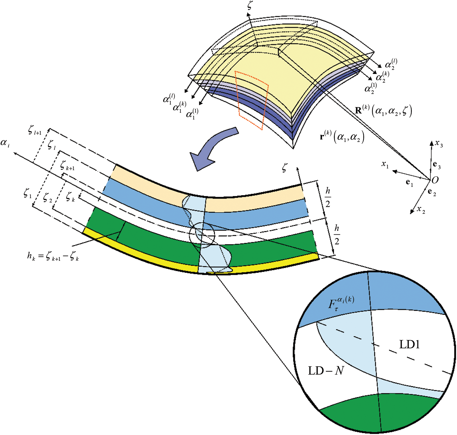
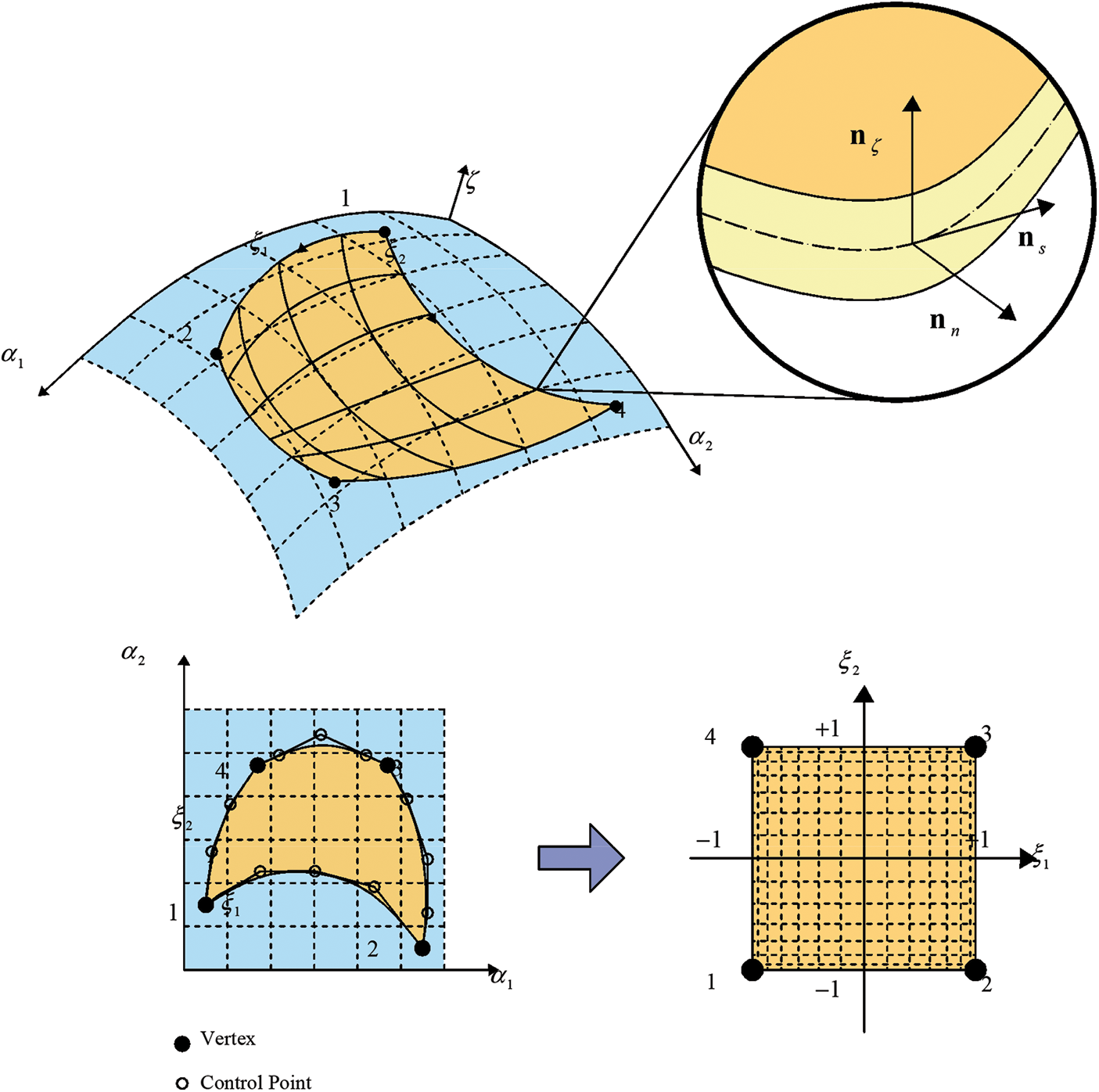
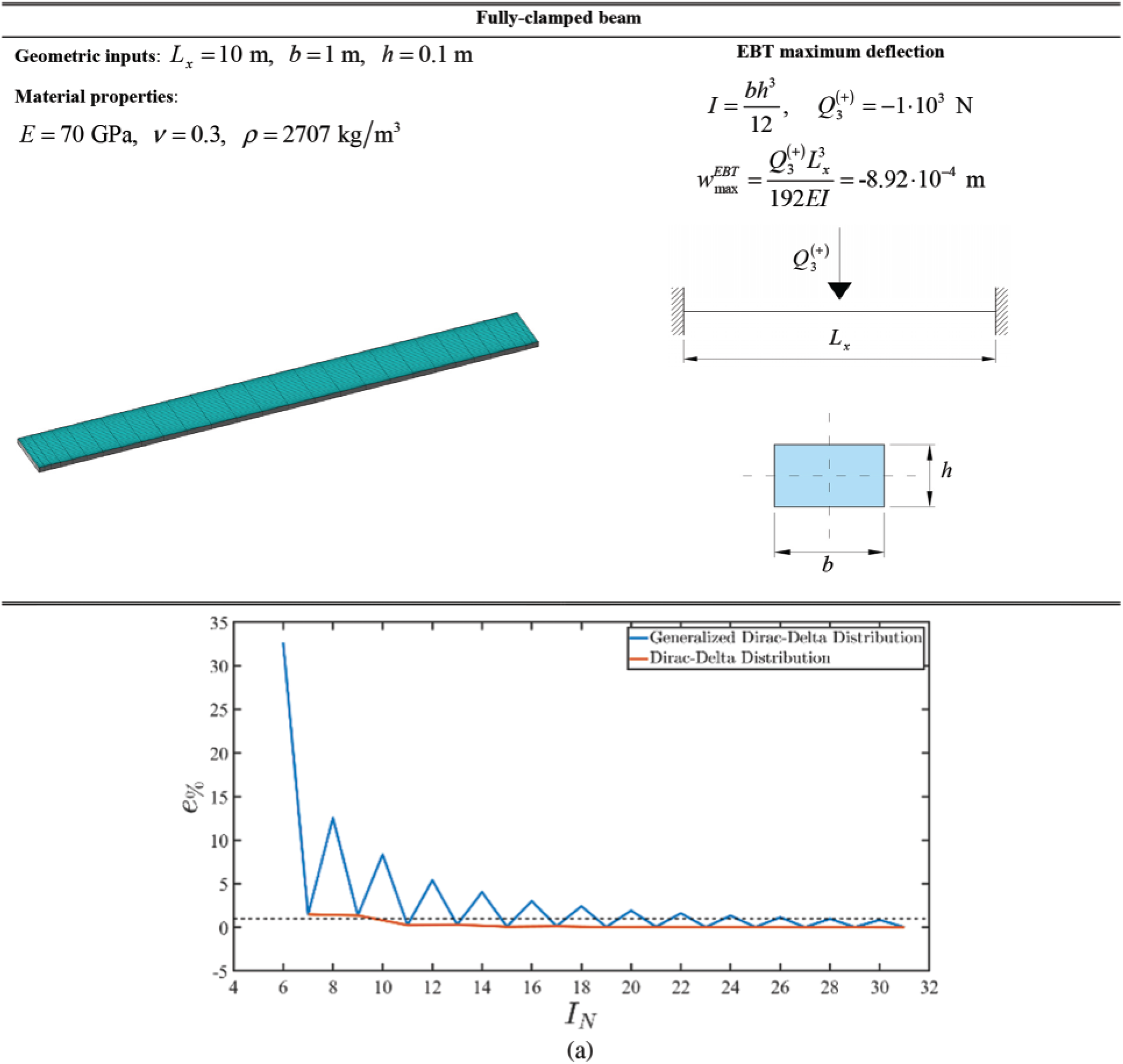
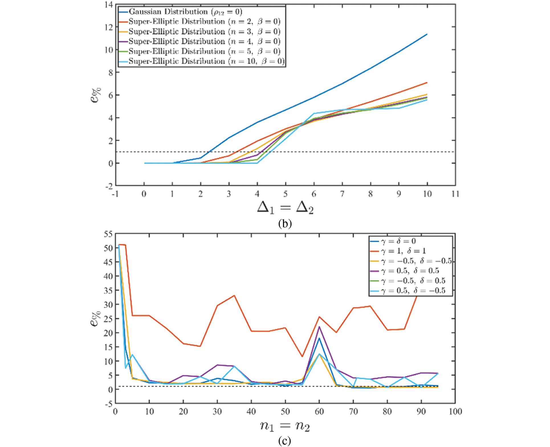
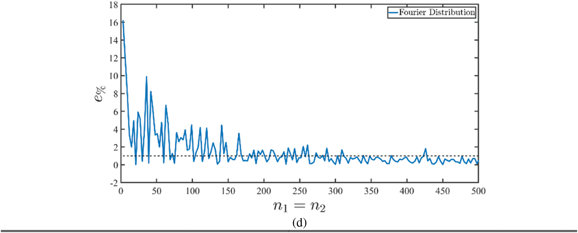
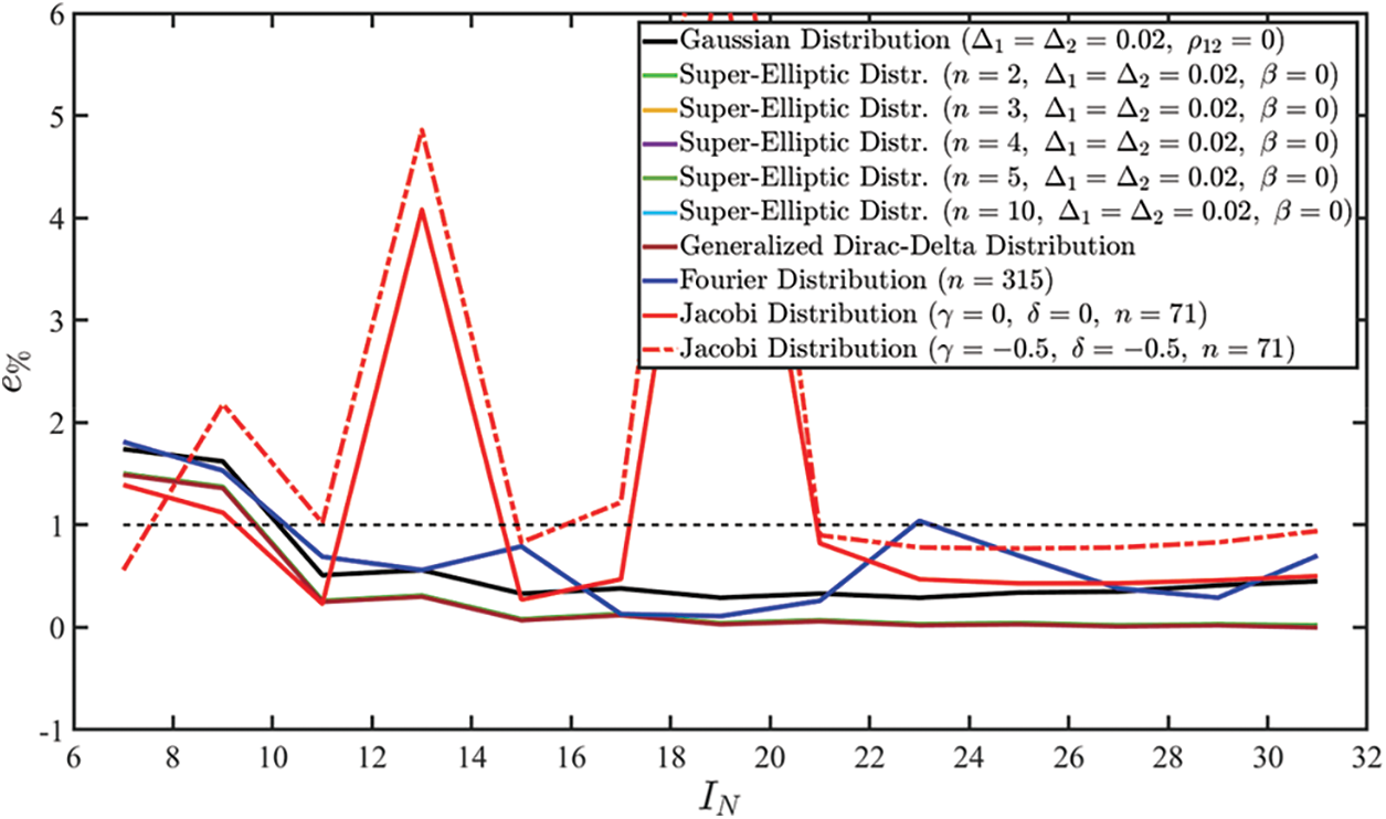
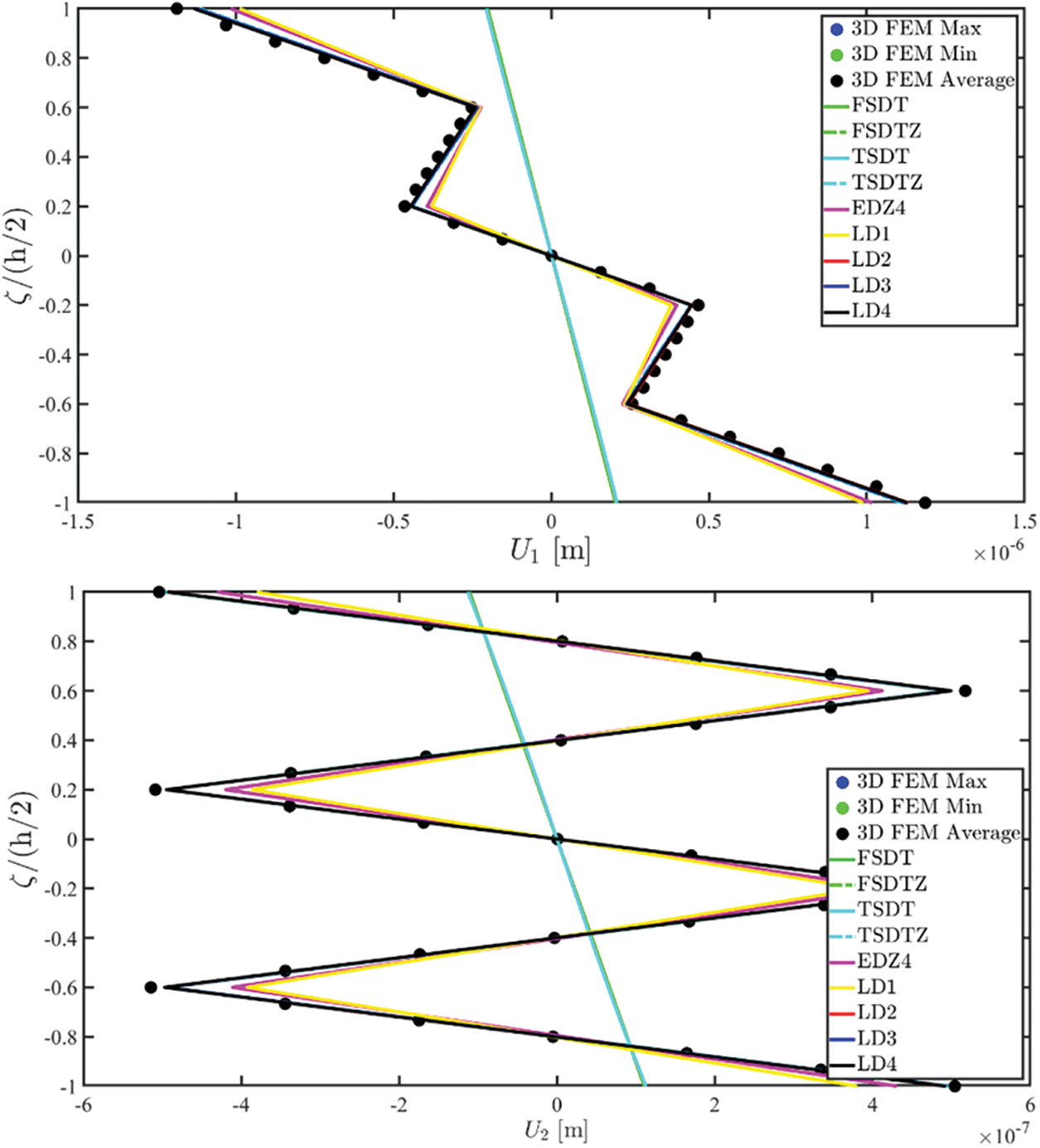
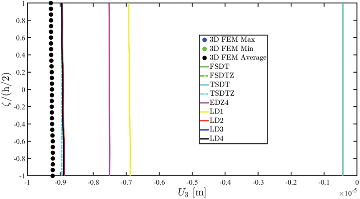
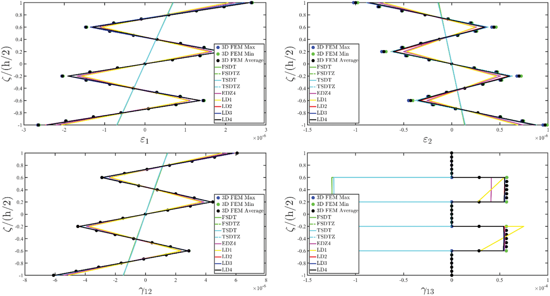
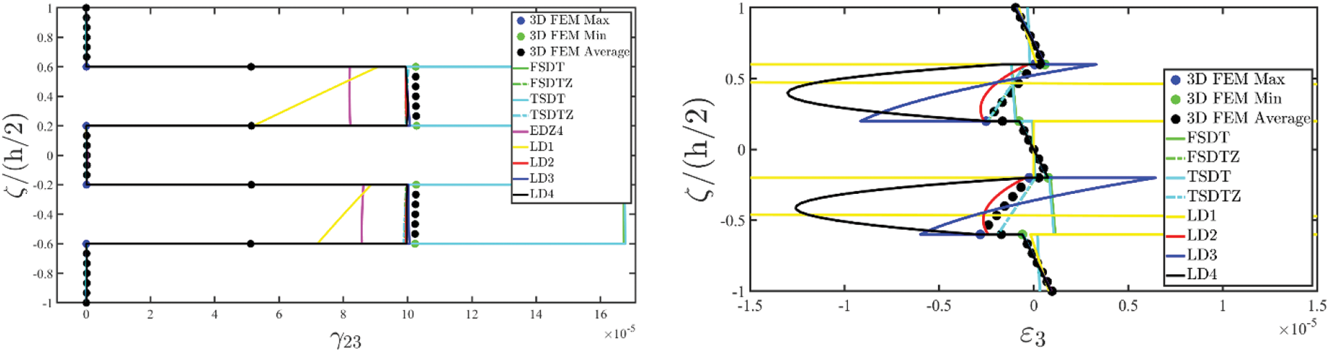
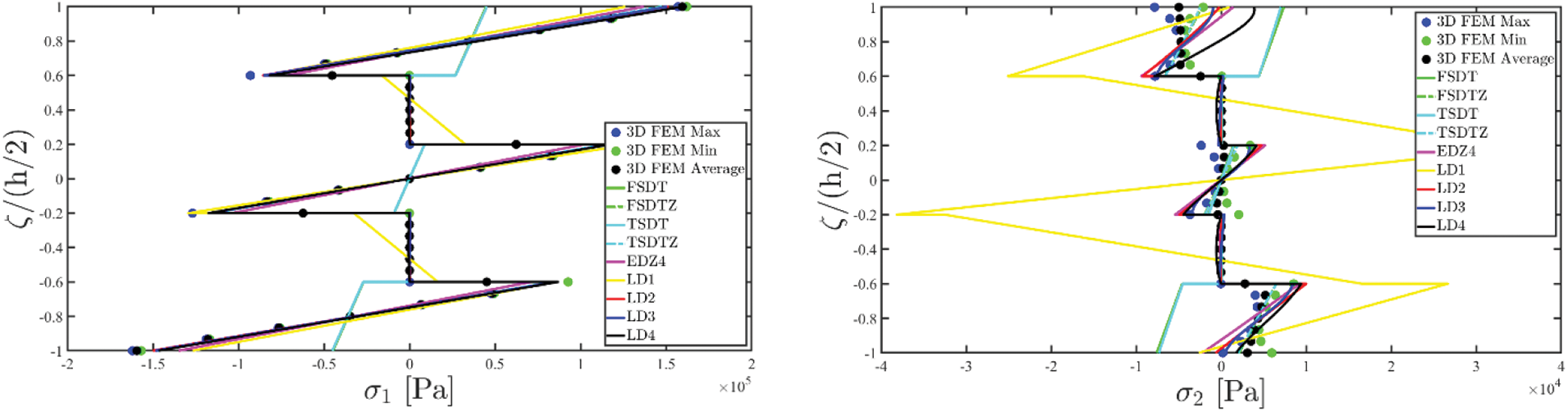
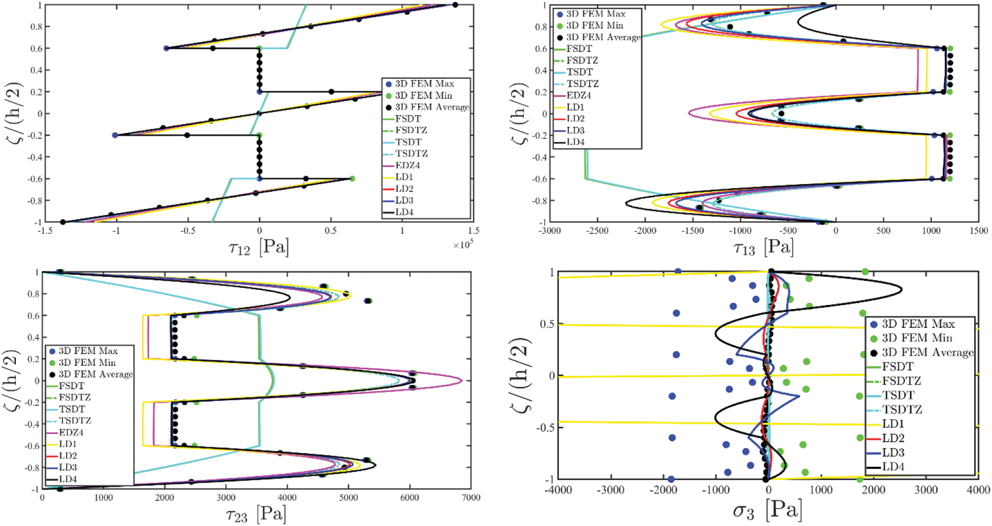
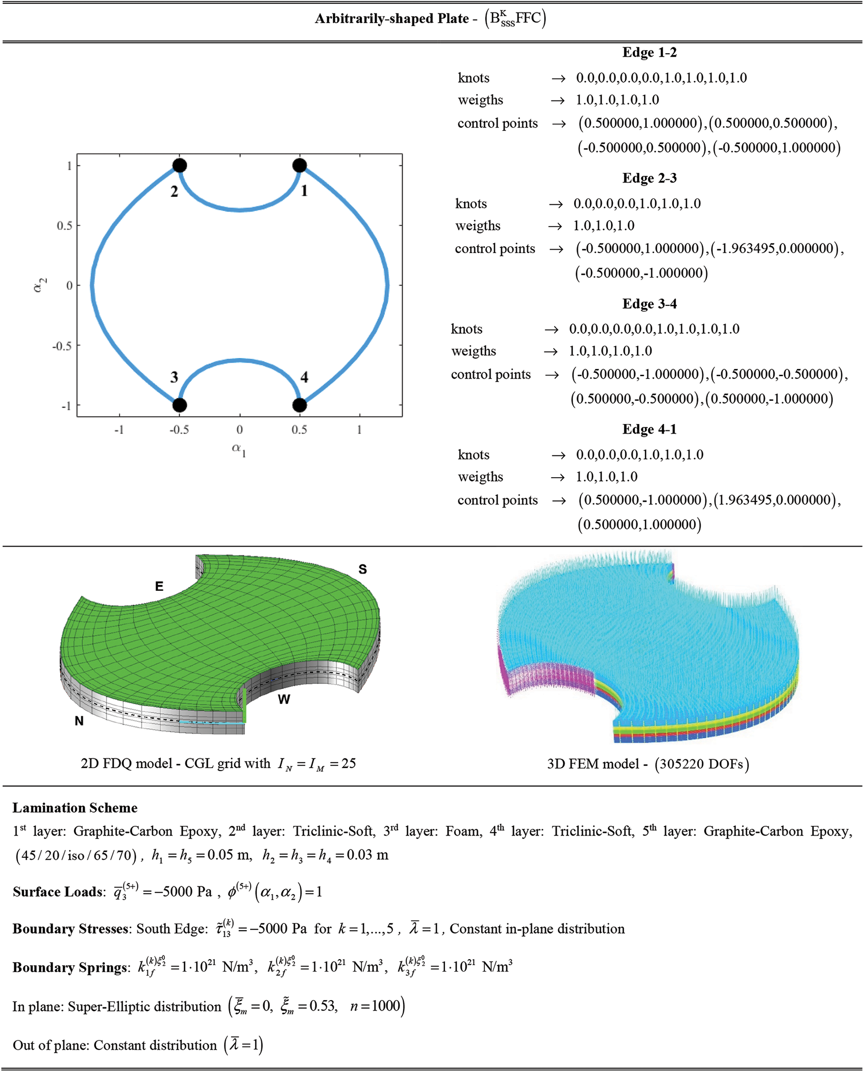
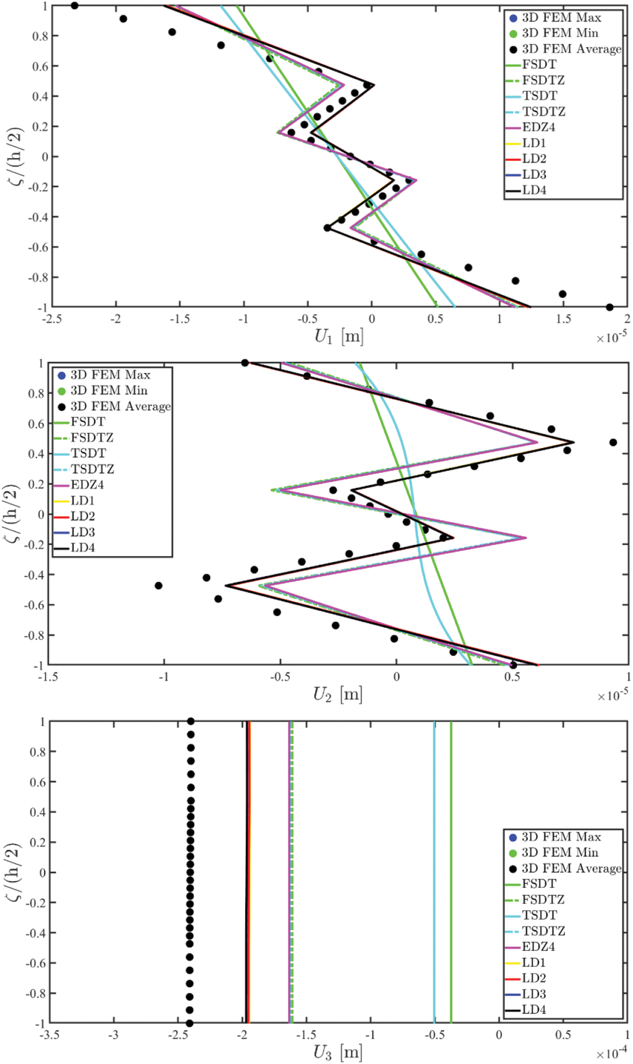
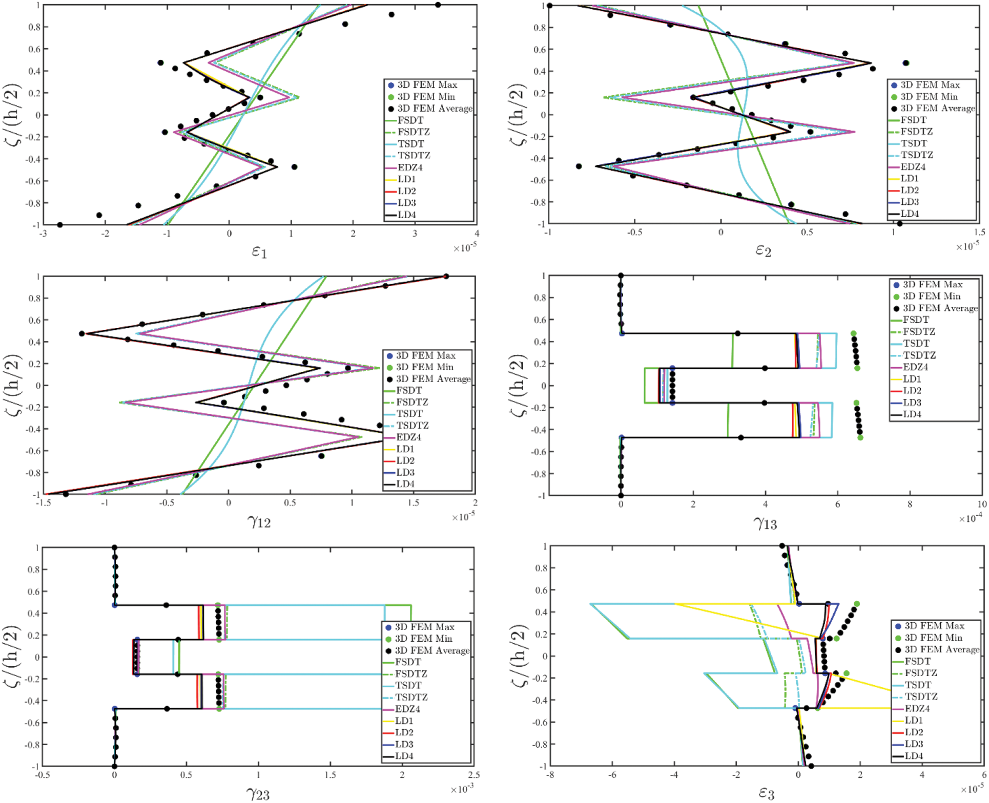
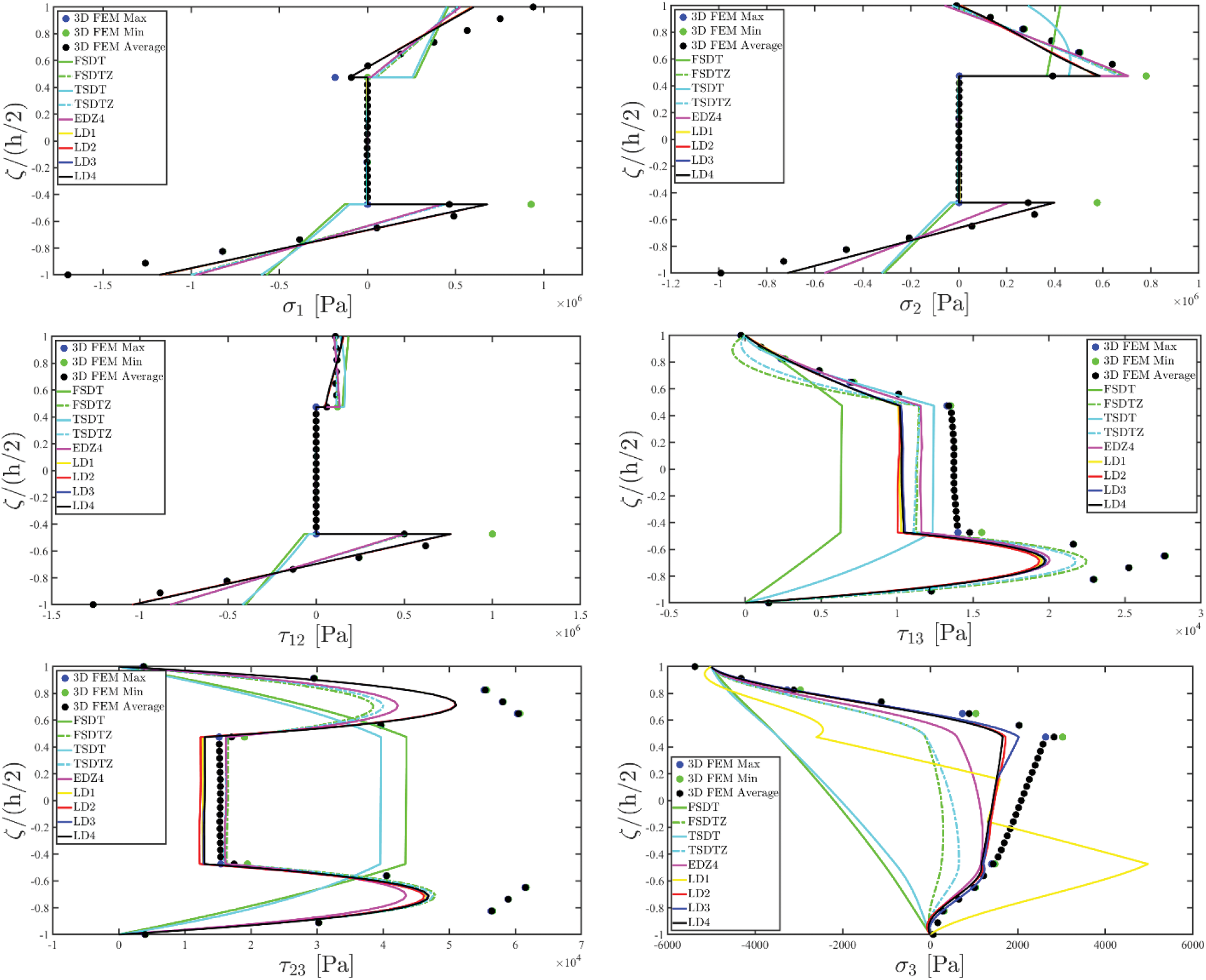
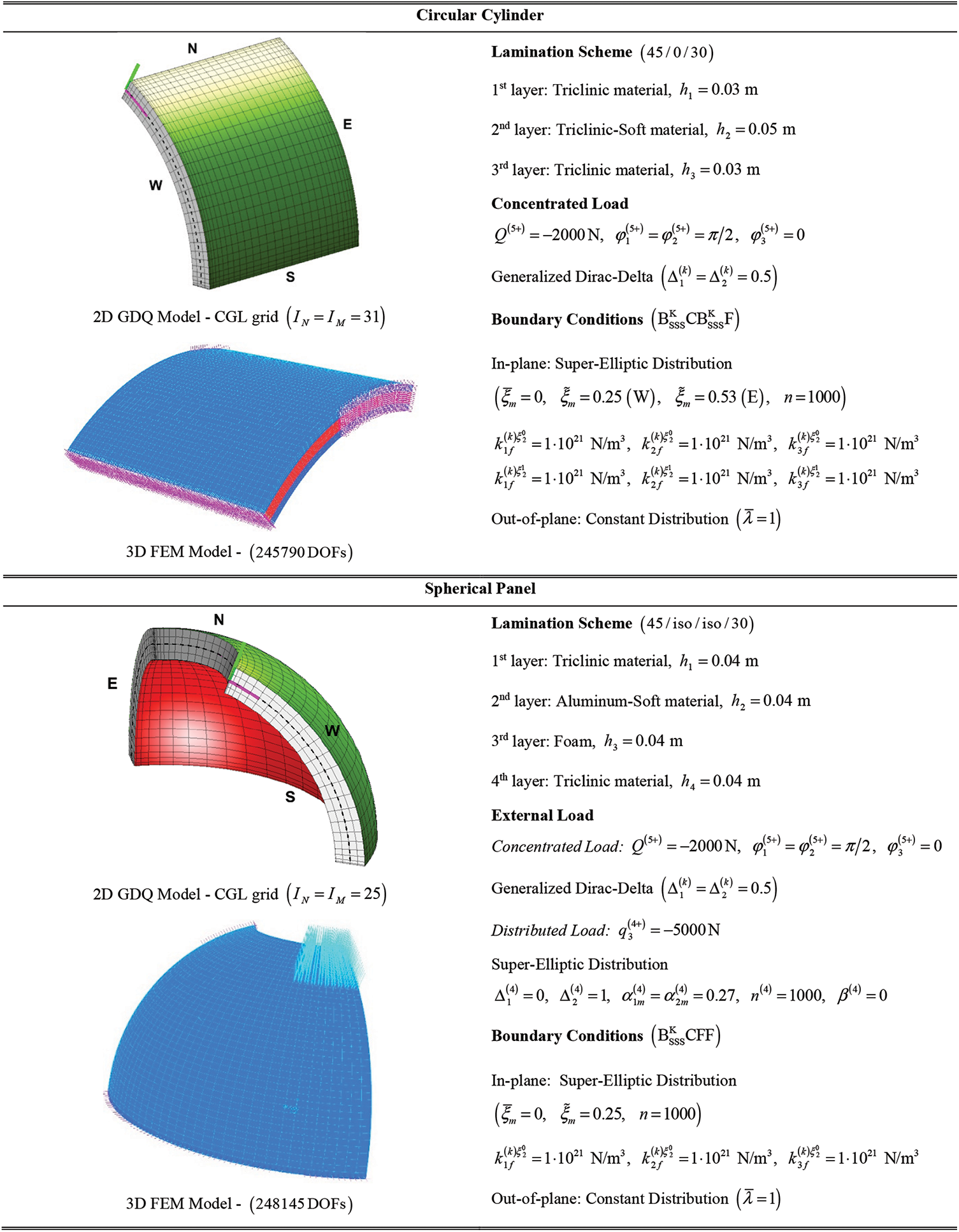
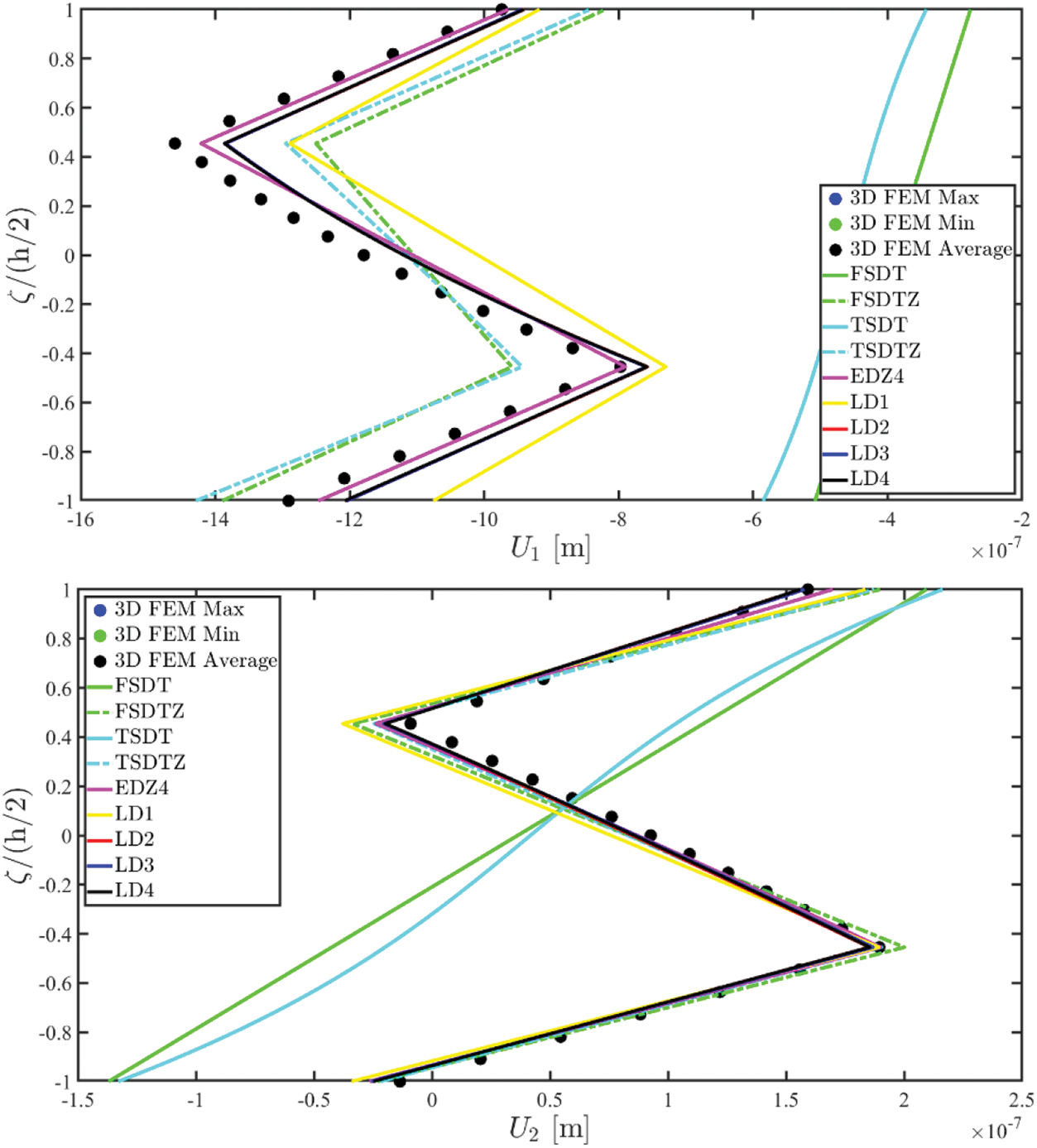
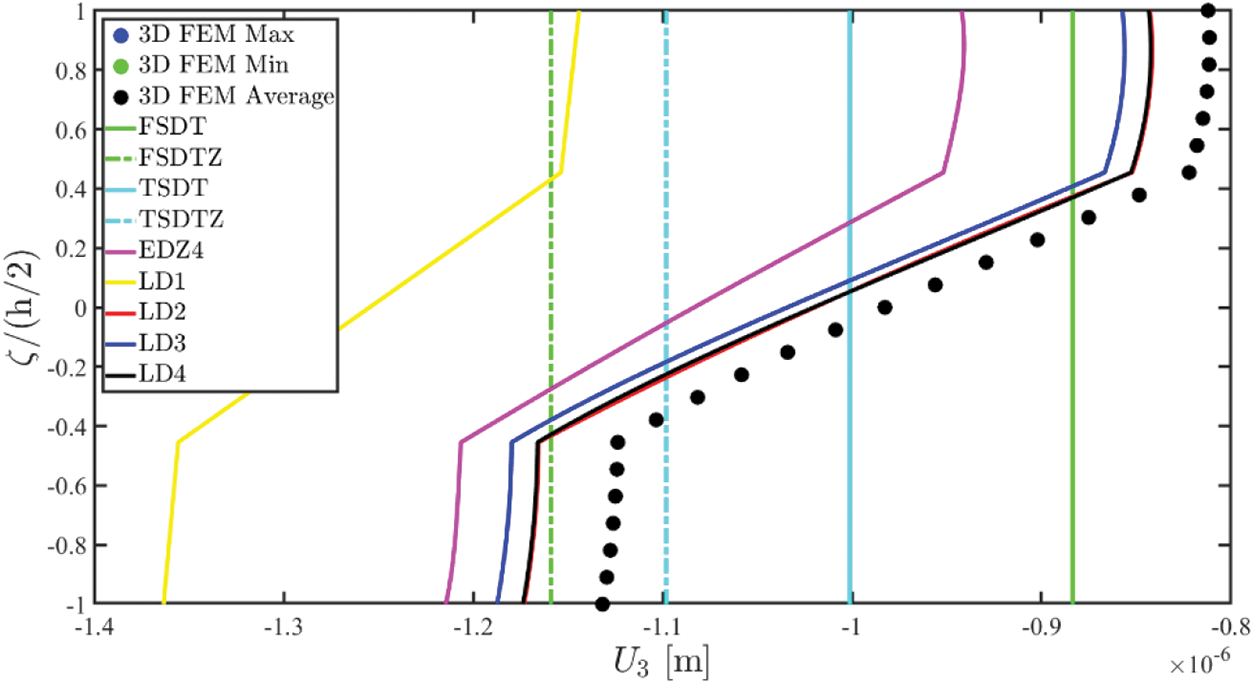
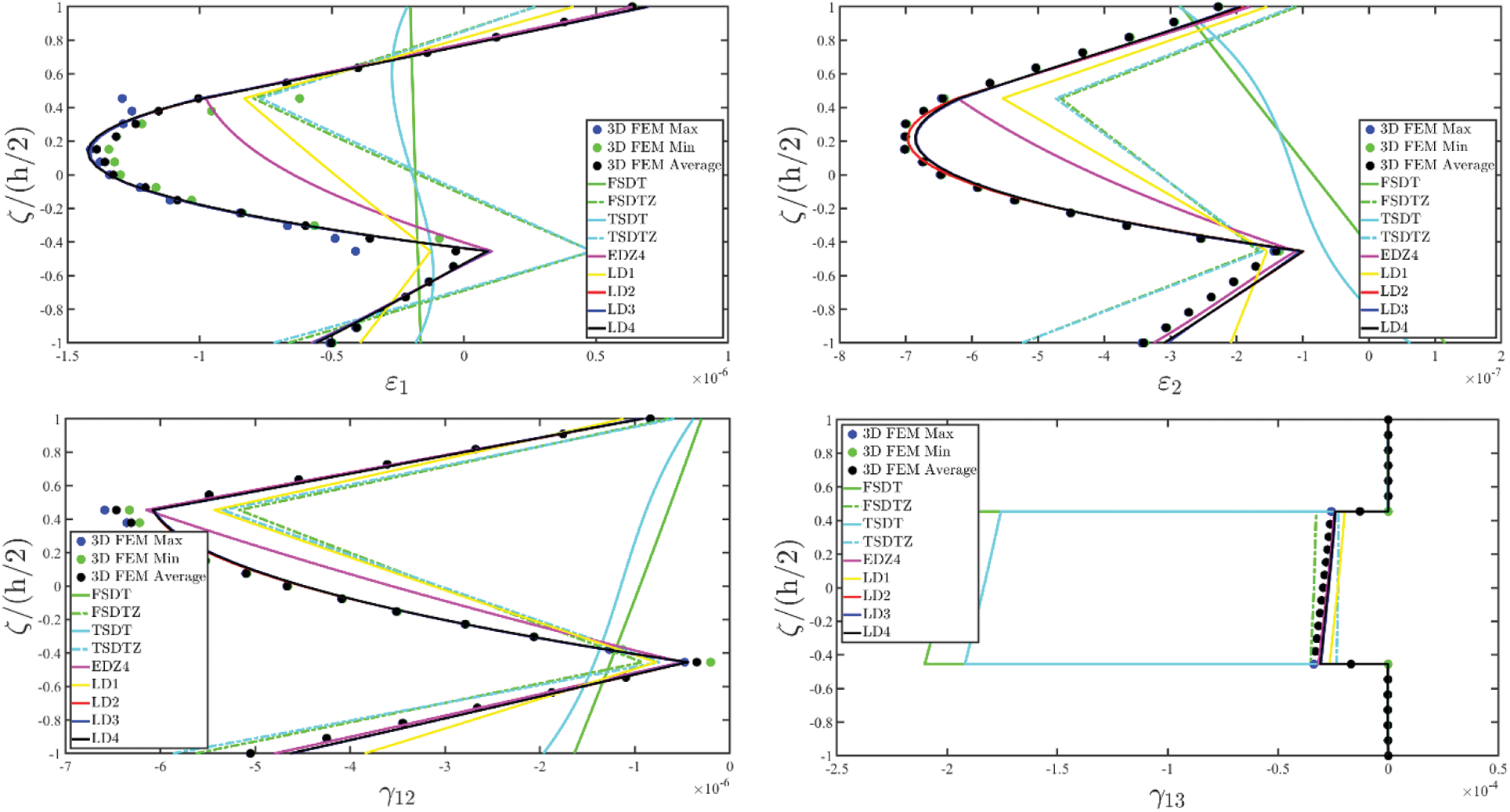
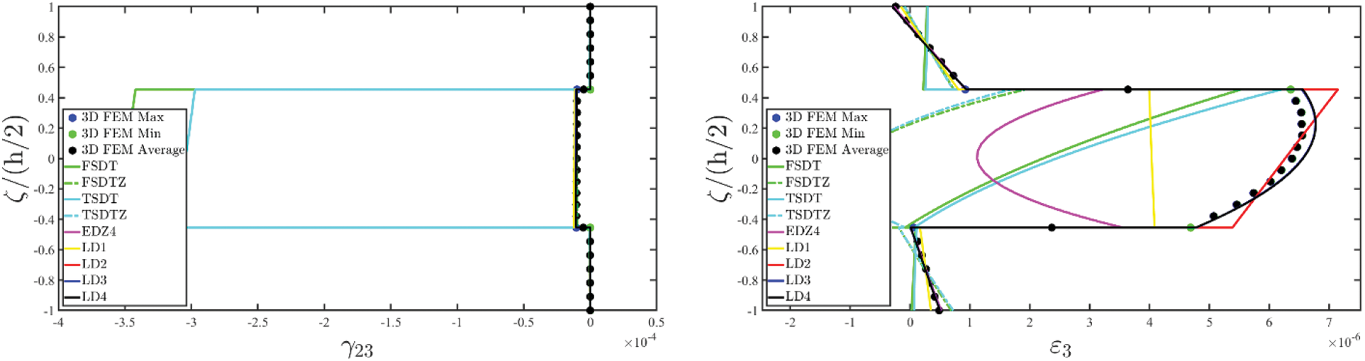
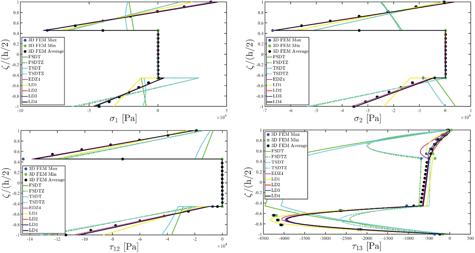
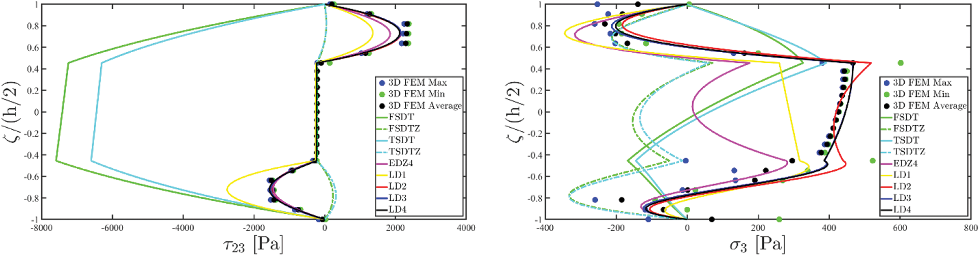
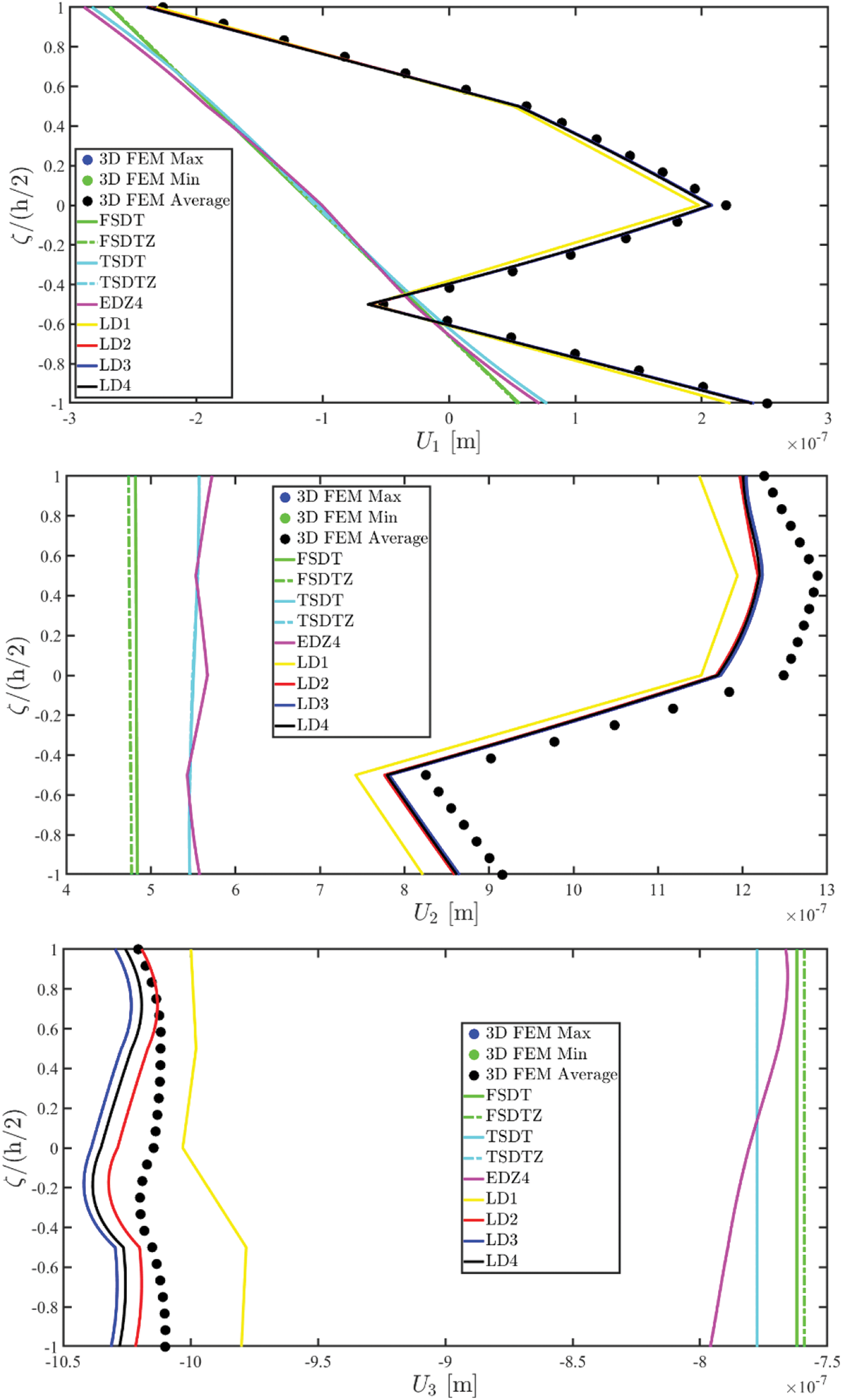
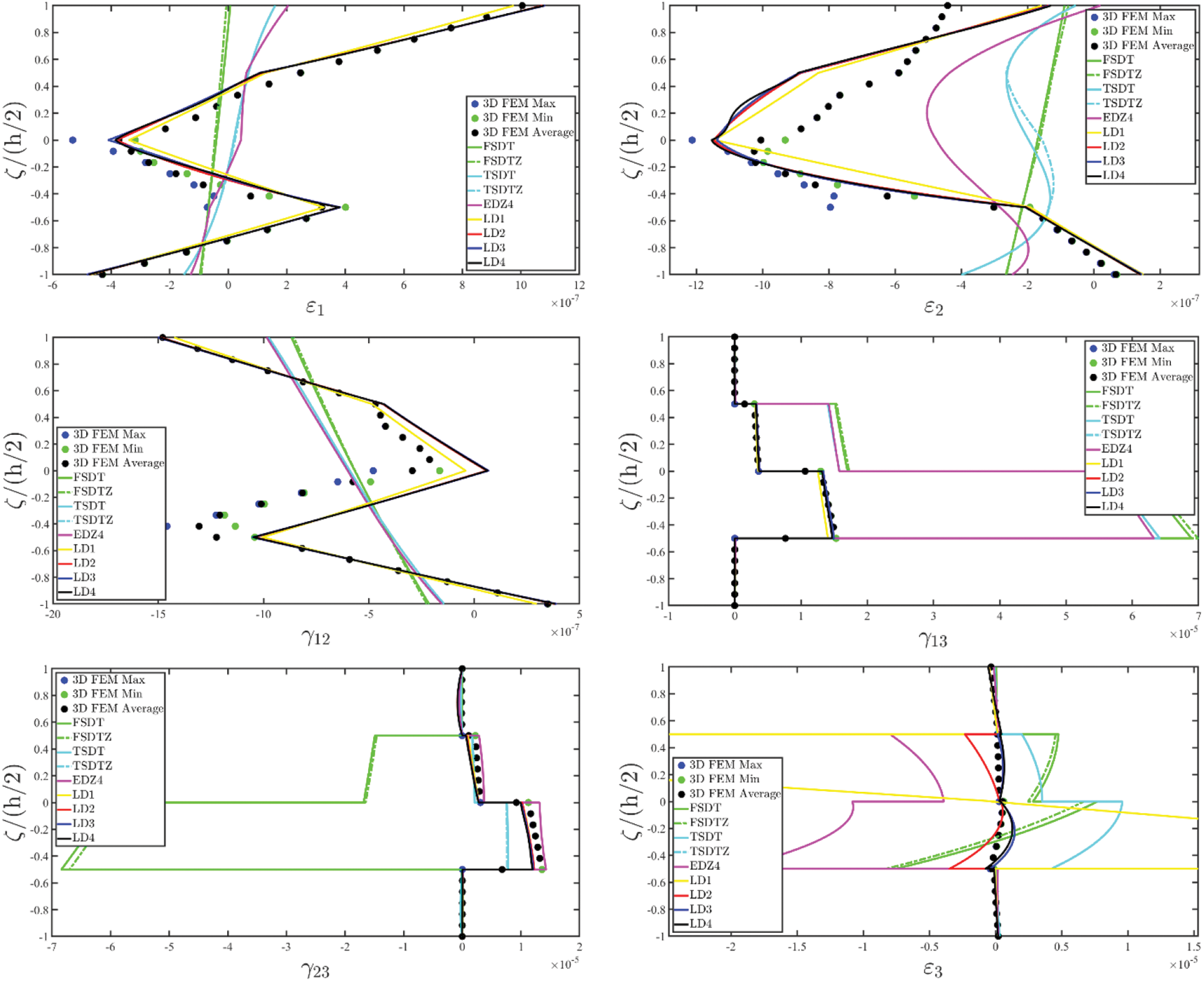
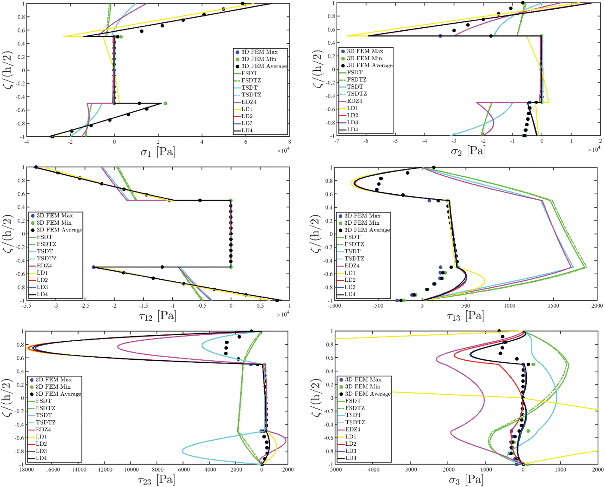
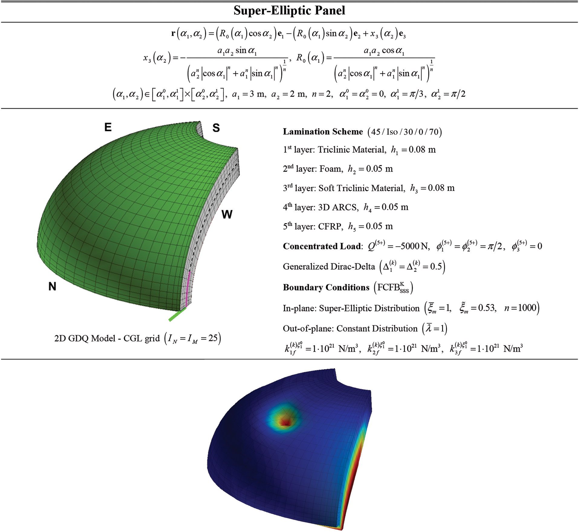
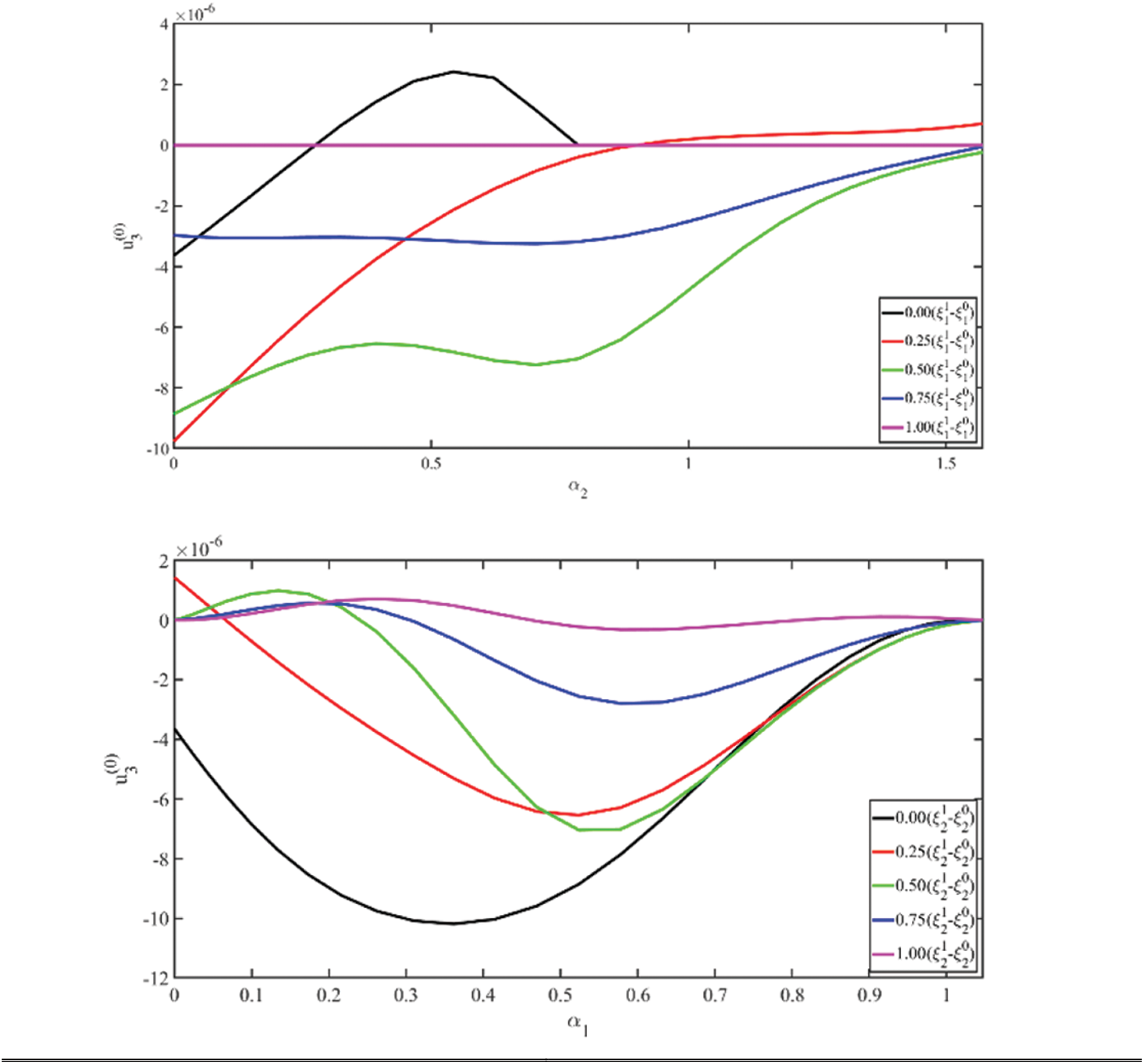
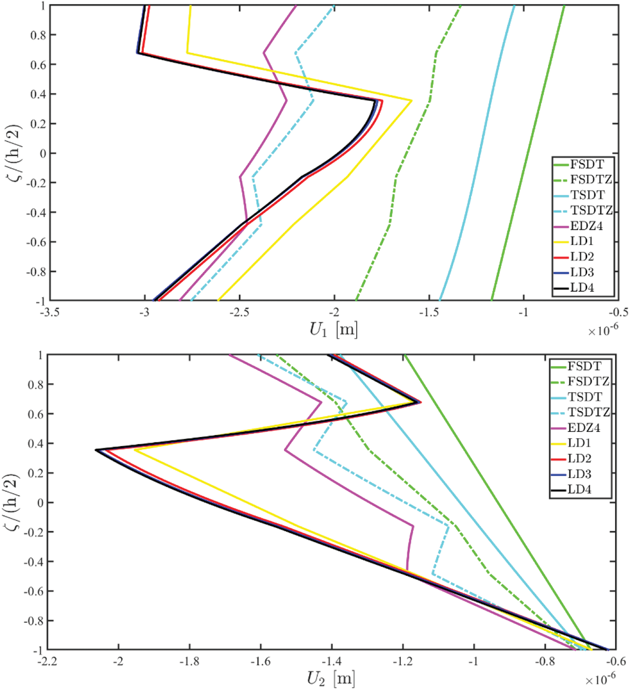
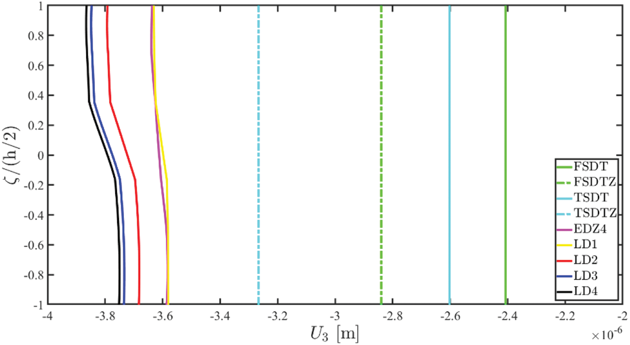
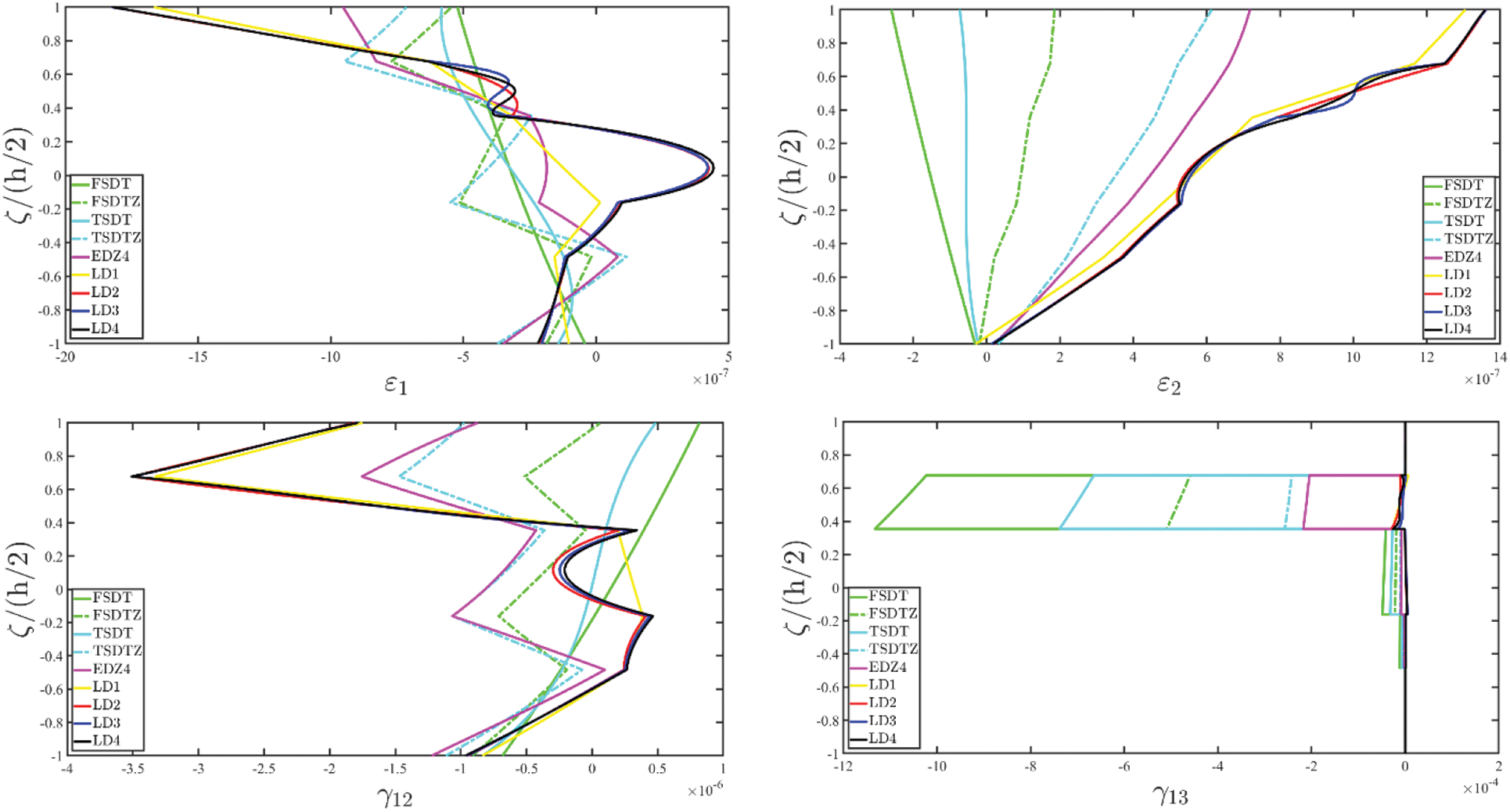
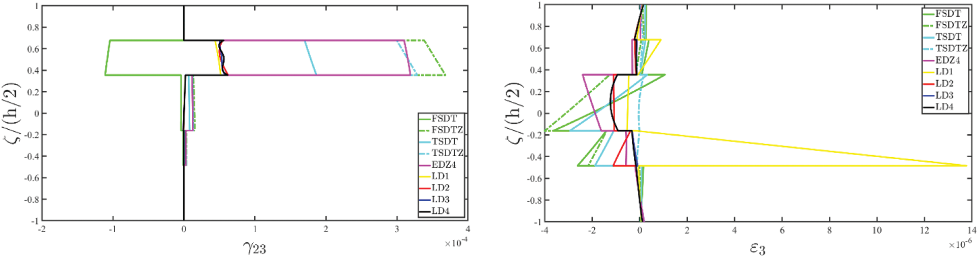
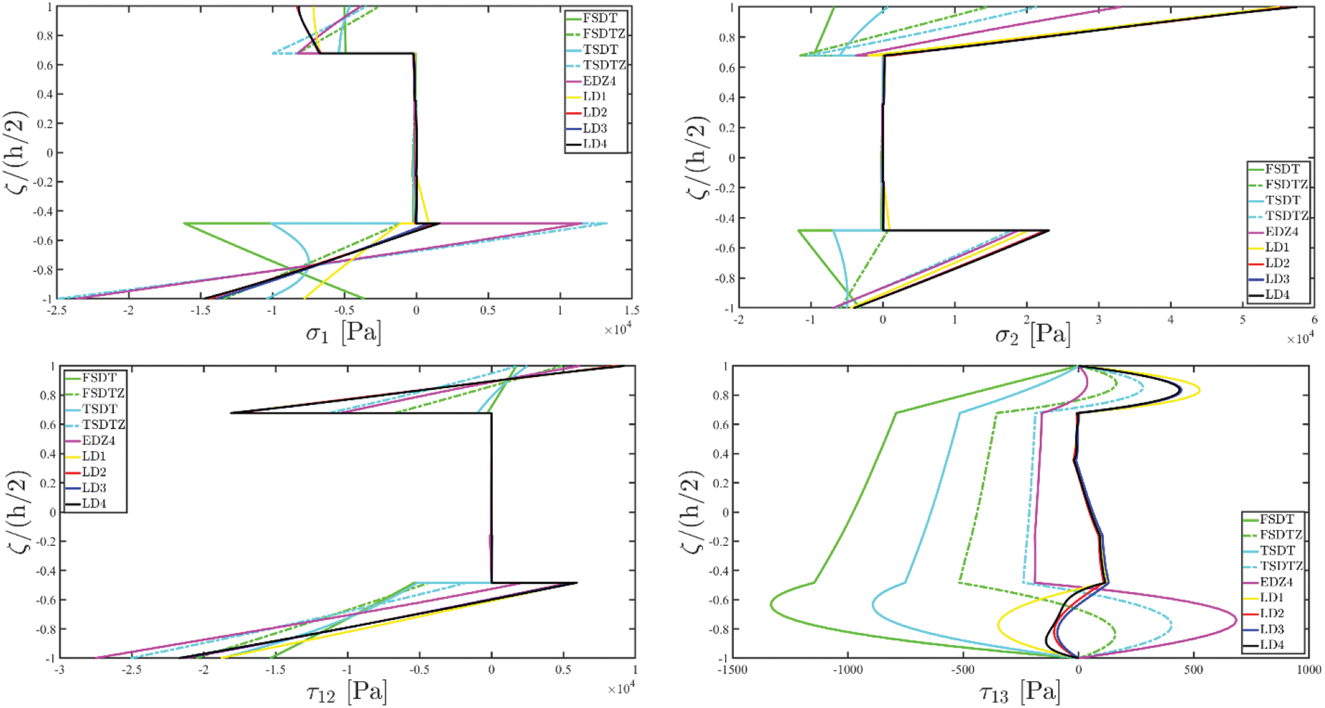
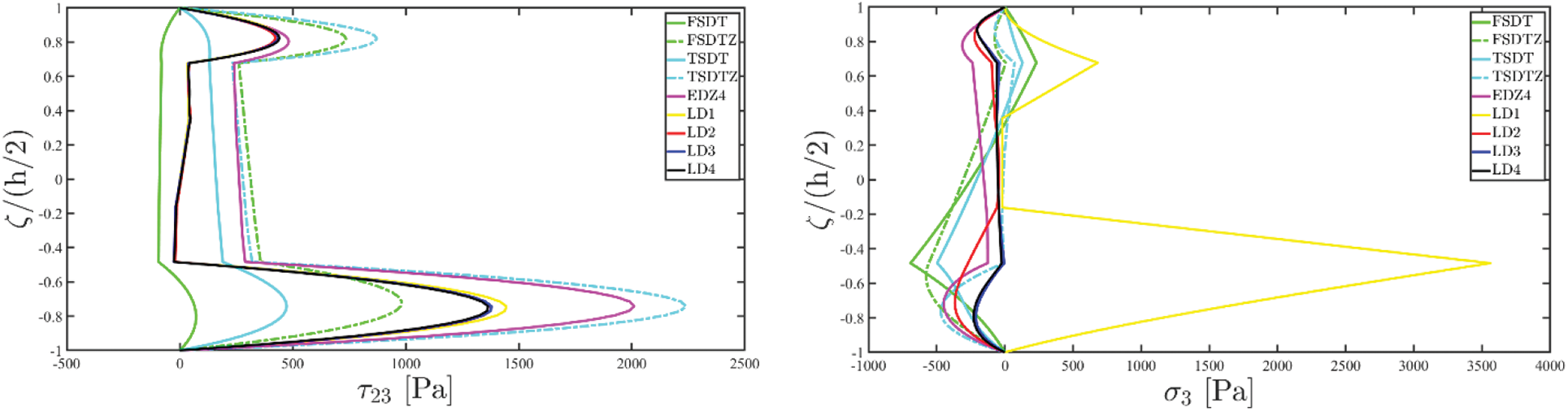
 Copyright © 2023 The Author(s). Published by Tech Science Press.
 Downloads
 Citation Tools