Multi-Objective Redundancy Optimization of Continuous-Point Robot Milling Path in Shipbuilding

1  Introduction

Recently, industrial robots have been widely used in simple repetitive tasks such as palletizing due to the advantages of large working space, strong flexibility, and low energy consumption. The geometry and surface quality of free edges of hull parts are required in PSPC for shipbuilding. The traditional shipbuilding industry uses grinding to process the free edges of parts, but this machining method is inefficient and wasteful of labor.

CNC machining or robot milling can also be used to machine the free edges of hull sections. However, only a few industrial robots are employed in five-axis milling, owing to the complexity of robot programming for continuous machining compared to simple repetitive operations.

In the robot milling application, the trajectory of the end effector (EE) is usually converted from the cutter location (CL) data, which is generated by the computer-aided manufacturing system (CAM) software. The typical cutter location data usually requires five degrees of freedom, three of which represent the coordinates of the tool center point (TCP) and the other two represent the direction of the tool axis. However, the standard industrial robot usually has 6 degrees of freedom, which will cause that there is a redundant DOF when the industrial robot is used for five-axis milling.

There are usually two methods to deal with the redundant DOF. The first method is to make the spindle coaxial with the last joint of the industrial robot when it is installed, as shown in Fig. 1. This method reduces the robot’s degrees of freedom to five, allowing the redundant DOF to be ignored while milling path planning. Another method, the most popular method, is mounting the spindle and the last joint axis of the wrist non-collinearly to improve the dexterity and manipulability of the robot, as shown in Fig. 2. The second method provides an opportunity to optimize the path given a specified CL [1]. Therefore, the redundancy optimization becomes a major issue in path planning of robot milling.

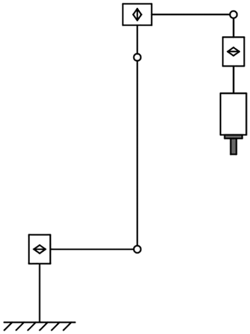
Figure 1: The milling robot whose last joint is coaxially mounted with the spindle

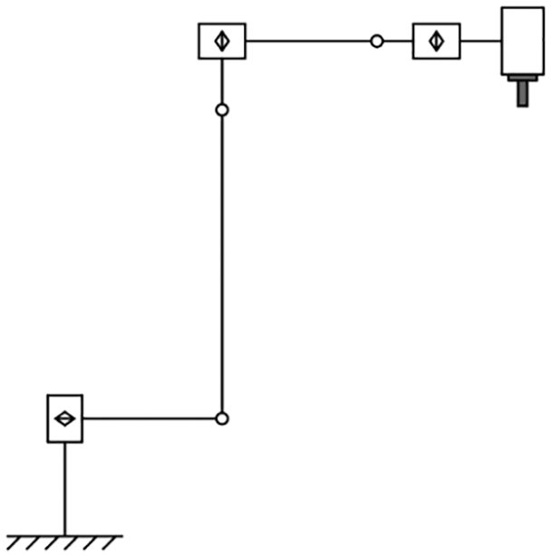
Figure 2: The milling robot whose last joint is not coaxially mounted with the spindle

Recent studies on the redundant resolution of the industrial robot have proposed many different performance indexes, such as energy [2], smoothness [3], joint torque [4], processing time [5]. Zhang et al. proposed energy objective function by the use of dynamic model and Lagrangian formalism [2,6]. Based on the velocity and acceleration of the joints, Dolgui et al. [7] proposed an energy objective function and an optimization algorithm for the redundant resolution of robotic laser cutting. On the basis of Alexandre’s research, Zhang et al. [3] established a new energy evaluation function by using the numerical difference of velocity and optimized the path generated by Alexandre’s algorithm even more. Zhang et al. [4] proposed the velocity-level and acceleration-level redundancy resolution schemes to minimize the joint torque of functional redundant industrial robot. Al Khudir et al. [5] established the objective function of the optimization algorithm at the acceleration level to minimize the motion time. All of the studies mentioned above are single-object redundancy optimization. But there are multiple requirements for the machining performance in the actual robot machining application. Single-objective redundancy optimization is not suitable for real robot machining. It is necessary to apply the multi-objective redundancy optimization according to the actual requirement of machining performance. In terms of algorithm, Zhang et al. used the quadratic programming algorithm to optimize the objective function [2,4]. Dolgui et al. [7] proposed a redundancy optimization algorithm based on the Graph-based method. Peng et al. [3] used the sequential linearization programming method to accomplish the continuous-point path planning. Doan et al. [8–10] selected the PSO algorithm to optimize the redundancy of the robot. Ruiz et al. [1, 11–13] applied the GA algorithm to redundancy resolution. Most of the previous studies were focused on single-point sequential optimization or short continuous-point optimization, which are not suitable for continuous-point milling path planning. Since the optimization results of each point affect each other, single-point sequential optimization cannot obtain the global best solution for continuous-point path planning. The dimension of the heuristic algorithm increases as the number of points in the trajectory increases, the higher the dimension, the lower the efficiency of the algorithm.

As previously stated, previous research on industrial robot redundancy optimization has the following shortcomings:

1.    Most research was aimed at single-objective optimization, which is not suitable for actual robot milling.

2.    Some solved the multi-objective optimization by putting weights on the objective function, but the values of the weights are difficult to determine. Besides, the quality of the solution is difficult to be guaranteed.

3.    Most research was aimed at single-point posture optimization or fewer points optimization, but the milling path contains multiple continuous points.

4.    The existing methods for the continuous points path optimization of the redundant robot are not universal for paths consisting of different numbers of points.

During the ship construction, a large number of free edges need to be polished to meet coating requirements. The machining path generated by CNC software consists of multiple points. As a result, the multi-point path planning is more suitable for the milling tasks in shipbuilding. Apart from this, the multi-point path planning can avoid the point-by-point deterioration of the robot pose since it is global optimization considering the entire path. As a result, the optimization algorithm based on multi-point path planning makes it easier to obtain a trajectory with improved smoothness and manipulability, which can improve shipbuilding efficiency.

Owing to the above reasons, the challenge of robot path planning is to put forward an algorithm aimed at multi-objective redundancy optimization of continuous points, which is suitable for any number of points. To solve this problem, this paper proposed a new redundancy optimization algorithm based on the DE and NSGA-Ⅱ algorithm. First of all, by analyzing the functional redundancy of the robot, the relationship between redundant DOF and machining path was determined. Then we established the optimization model which took the smoothness performance, energy performance, joint-limit, and singularity avoidance into consideration. An optimization method based on DE and NSGA-Ⅱ was proposed to solve the optimization problem. The optimization algorithm can obtain satisfactory optimization results while avoiding the impact of the number of points.

The remainder of this paper is organized as follows. In Section 2, the formula which presents the relationship between the redundancy and the CLs is given. In Section 3, the optimization which contains the energy performance index and the smoothness performance index is proposed. In Section 4, the redundancy optimization algorithm based on DE and NSGA-Ⅱ is developed. In Section 5, simulations are conducted to confirm the validity of the proposed approach. Section 6 concludes the paper.

2  Redundancy in the Application of Robot Milling

Fig. 3 shows the application of five-axis robot milling. In Fig. 3, the {TCP} presents the coordinate system of the tool center point, and {WCS} represents the world coordinate system. The CLi denotes the cutter location of the ith point in the milling path. The CL data is usually generated by the CAM software, it can be expressed as CL(x, y, z, i, j, k), in which (x, y, z) is the coordinate of the cutter in {WCS} and (i, j, k) is the unit vector of the cutter axis.

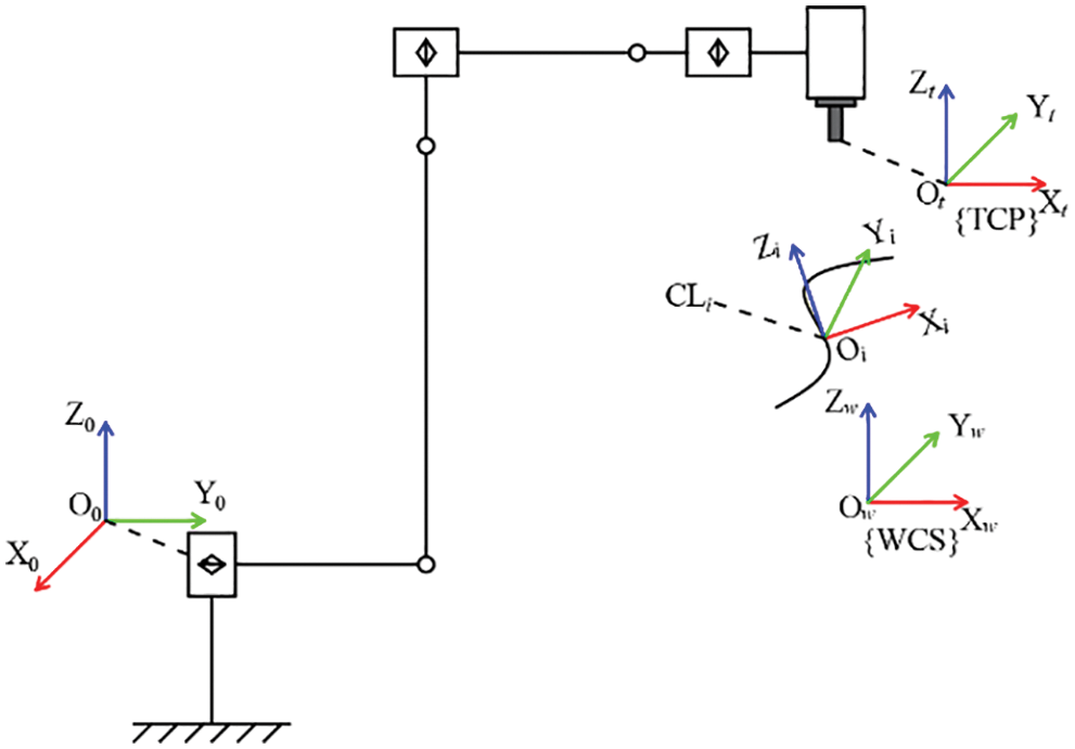
Figure 3: The application of five-axis robot milling

It is easy to know from Fig. 3 that the rotation of TCP around the cutter axis does not affect the milling task because it will not change the direction of the cutter axis. But the rotation of TCP will result in a change in the robot’s posture. Rotation of different angles will cause different postures, and different robot postures will cause different robot performance.

Let the six-dimensional vector (x, y, z, α, β, γ) represents the posture of EE of the robot (in this paper, the EE means the milling cutter), the (x, y, z) represents the location of EE and the (α, β, γ) represents the Euler Angles.

Attach the TCP frame to the cutter, with its origin at the TCP and its z-axis coinciding with the cutter axis. So the frame transformation of {TCP} relative to the {WCS} can be described by the posture of EE (x, y, z, α, β, γ). According to the knowledge of coordinate system transformation [14], the transformation matrix wTt can be deduced as Eq. (1)

wTt=trans(x,y,z)rot(x,α)rot(y,β)rot(z,γ)=[cos⁡(β)cos⁡(γ)−cos⁡(β)sin⁡(γ)sin⁡(β)xcos⁡(α)sin⁡(γ)+sin⁡(α)sin⁡(β)cos⁡(γ)cos⁡(α)cos⁡(γ)−sin⁡(α)sin⁡(β)sin⁡(γ)−cos⁡(β)sin⁡(α)ysin⁡(α)sin⁡(γ)−cos⁡(α)sin⁡(β)cos⁡(γ)sin⁡(α)cos⁡(γ)+cos⁡(α)sin⁡(β)sin⁡(γ)cos⁡(α)cos⁡(β)z0001](1)

where trans and rot denote translational transform and rotation transformation, respectively. The 1st, 2nd, 3rd column of the matrix denotes the direction of axes of {TCP} and the 4th column denotes the coordinate of the origin of {TCP}. To perform the milling task, the cutter location should be equal to the 4th column of wTt. And the direction of the cutter axis should be equal to the negative of the 3rd of wTt, which can be written as Eq. (2)

[ijk0]=wTt[00−10](2)

It can be deduced that

[ijk]=[−sin⁡βcos⁡βsin⁡α−cos⁡αcos⁡β](3)

Eq. (3) shows that the CL data CL(x, y, z, i, j, k) is independent of the value of γ, which also proves the existence of the redundancy mathematically. So the main task of the path planning is to obtain an appropriate value of the redundancy DOF γ to ensure the data integrity of wTt. This can be realized via the optimization algorithm proposed by this paper.

3  Redundancy Optimization

3.1 Performance Indexes

It is clear from Section 1 that defining the appropriate performance for the redundancy optimization model is essential. In this paper, we choose the smoothness performance and energy consumption as the optimization objective, which are adjustable to the requirement of the processing task.

3.1.1 Smoothness Performance Index

A smooth speed curve in the milling process may not only efficiently assure machining accuracy and surface quality, but also satisfy the kinematics and dynamics constraints of the machining system. Vibration and jerk are the main factors affecting the smoothness of the milling path. Small joint angular acceleration can effectively avoid the velocity mutation, reducing vibration and jerk produced by the joint velocity control fundamentally. The feedrate is usually given in the design of the machining scheme. The angular velocity fluctuation of each joint during the machining process will cause spindle vibration and impact, and thus a massive change in feedrate, which will affect the smoothness of the machining path. Angular acceleration is an effective index to measure angular velocity fluctuation, it can be used as a performance index to measure the smoothness of trajectory. So the acceleration is chosen to evaluate the smoothness of the path.

For the milling path made up of n points, let θji denotes the angle variable of the jth joint at the ith point. In this paper, angular acceleration is selected to evaluate the smoothness of the path. But the accurate calculation of angular acceleration takes a lot of calculation. Interpolating the angle variable of each joint at each point and approximating the acceleration by the interpolation derivative formula is an effective method. According to the Newton interpolation method [15], the angular velocity can be written as Eq. (4)

wji={θji−θji−1△ti+△ti+1(θji−θji−1)−△ti(θji+1−θji)△ti+1(△ti+1+△ti)i∈(1,N−1]0i=1 or N(4)

and the angular acceleration can be written as Eq. (5)

aji={2ti+1(θji−θji−1)−ti(θji+1−θji)titi+1(ti+ti+1)i∈(1,N−1]0i=1 or N(5)

where wji, aji denotes the angular velocity and the angular acceleration of jth joint at the ith point respectively, ti=‖CLiCLi−1¯‖/v, where the v is the feedrate determined by CAM software. Different weights are used to indicate the effect of different joints on smoothness. So the performance index of smoothness for the path made up of N points can be written as Eq. (6)

Indexsmooth=maxi∈{2,…,N−1}⁡{ ∑j=16wj|aji|} (6)

where the wj denotes the weight coefficient. The more value of wj, the greater influence of jth joint on Indexsmooth is.

3.1.2 Energy Consumption Performance Index

According to the joint space dynamic model [14], the joint torque can be calculated as Eq. (7)

τ=B(q)q¨+C(q,q˙)q˙+g(q)+τf(q˙)+JT(q)he(7)

where the B(q) denotes the inertia matrix, C(q,q˙) denotes the matrix accounting for Coriolis/centrifugal effects, g(q) is the torque exerted gravitational force, τf(q˙) is the friction torque which is calculated as τf(q˙)=fcsgn(q˙)+fvq˙ with fc and fv the Coulomb and viscous friction coefficients, respectively, JT(q)he denotes the contact force.

There is little difference in motion time for different pathways when the milling feedrate is determined. So the energy consumption can be evaluated by the sum of the power at each point in the path, which can be calculated as Eq. (8)

Indexenergy=∑i=2N−1Pwri(8)

where the Pwri denotes the power of the ith point. The Pwri can be calculated as Eq. (9)

Pwri=∑j=16τjiwji(9)

Assume the optimization can achieve a low acceleration. The contact force in the robot milling application is always minimal and does not fluctuate across orders of magnitude as the pathways change due to the robot’s stiffness limit. Compared with the friction torque, the impact of gravity and the Coriolis effect in Eq.(7) is small. So Eq. (9) can be simplified to Eq. (10)

Pwri∼∑j=16(wji)2(10)

which is called Minimum Velocity Norm (MVN) Scheme. And this scheme has been proved effective in energy-saving optimization [4]. The execution of MVN Scheme only needs to calculate angular velocity without dynamic modeling, which can only conduct a qualitative analysis of energy consumption but greatly improves the calculation speed of the optimization algorithm, and it is enough for the optimization.

3.2 The Constraints

Near the singularity, to make the EE achieve the desired speed, the joints must rotate at a very high speed [16], which should not occur in the milling task. The robot posture should be far away from the singularity to maintain suitable manipulability during milling. The further the posture is away from the singularity, the better the manipulability of the robot.

Write the Jacobian in the form of a partitioned matrix, the speed vector of EE can be calculated as Eq. (11)

[p˙EωE]=[J11OJ21J22][q˙1−3q˙4−6](11)

where the p˙E and the ωE denote the linear velocity and the angular velocity of EE, respectively, the q˙1−3 and the q˙4−6 denote the angular velocities of the first three joints and the last three joints, respectively. We can obtain Eqs. (12) and (13) from Eq. (11) that

q˙1−3=J11−1p˙E(12)

q˙4−6=J22−1(ωE−J21q˙1−3)(13)

According to the knowledge of coordinate transformations, Eq. (12) can be changed into Eq. (14)

q˙1−3=J11−1p˙E=3J11−1⋅3p˙E(14)

where the 3J11−1 and the 3p˙E denotes the Jacobian and the speed in joint frame{3}, and 3J11=(03R)−1J11. J11 can be obtained by vector product method [14] as Eq. (15)

J11=[−a3s1c23−a1s1−a2c2s1−d4s1s23−c1(a2s2−d4c23+a3s23)−c1(a3s23−d4c23)a1c1+d4c1s23+a2c1c2+a3c1c23−s1(a2s2−d4c23+a3s23)−s1(a3s23−d4c23)0s23d4+a2c2+a3c23s23d4+a3c23](15)

So the 3J11−1 can be calculated as Eq. (16)

3J11−1=[1k10001k20001k2][0−10−a30−d4a3+a2c30d4+a2s3](16)

where

{k1=a1+a3c23+d4s23+a2c2k2=a2(d4c3−a3s3)(17)

It is easy to know that the q˙1−3 cannot be calculated when the singular factor k1=0 or k2=0 as Eq. (17). Using the same method as above, the 5J22−1 can be calculated as Eq. (18)

5J22−1=J22−1(05R)=1k3[−1000k30c50k3](18)

where k3=s5. k3 is another singular factor.

The robot is at the singularity when the singular factor k1=0 or k2=0 or k3=0. So the constraints of singularity can be written as Eq. (19)

{|k1|≥δ1|k2|≥δ2|k3|≥δ3(19)

where the δ1, δ2, δ3 are the critical value for singularity avoidance. The constraint based on the singular factor can avoid solving the Jacobi matrix to reduce the computation of the algorithm.

The constraint based on the hardware of the robot usually contains the joint limit and the adjacent linkage interfere constraint.

The joint limit can be obtained from the parameters of the robot as Eq. (20)

BL≤q≤BH(20)

where the BL, q and BH denotes the vector of joint low bound, the vector of the joint angular variable, and the vector of joint high bound, respectively.

To avoid linkage interference of adjacent linkage, this paper proposed another constraint, which can be written as Eq. (21)

θj−θj−1∈[θjl,θjh](21)

where the [θjl,θjh] denotes the relative motion interval that guarantees non-interference.

3.3 The Optimization Model

Take the redundancy DOF vector γ as an optimization variable and find the suitable γi in the interval [−π,π] to achieve the optimization goal at the ith point. Once the variable γi is determined, the transformation matrix wTt can be calculated by Eq. (1). And the transformation matrix of the 6th joint relative to {B} can be calculated as Eq. (22)

BT6=BTWWTTTT6(22)

where the BTW and TT6 denote the be obtained by the transformation matrix of {B} relative to {WCS} and the transformation matrix of the 6th joint relative to {T}, respectively, which can be obtained by the layout of the workspace. The WTT can be obtained by the CL data.

The joint variable vector q can be calculated in Eq. (23)

q = ik(BT6)=ik(BTWWTTTT6)(23)

where the ik(⋅) means the inverse kinematics function.

The optimization model can be expressed as Eq. (24)

min.y=f(γ)=[Indexsmooth(γ),Indexenergy(γ)]s.t.{q = ik(BTWWTTTT6)γi∈[−π,π]i=1,2,…,NBL≤q≤BHθj−θj−1∈[θjl,θjh]|k1|≥δ1|k2|≥δ2|k3|≥δ3(24)

4  Optimization Algorithm

4.1 The Non-Dominated Sorting Genetic Algorithm II

The NSGA-II algorithm (Non-dominated Sorting Genetic Algorithm II) was put forward by Deb et al. [17], it is commonly used in multi-objective optimization. The algorithm stratifies the population by Pareto dominance relation and increases the population diversity by calculating the crowding distance.

In the minimizing multi-objective optimization problems, for the n-objective function f1(X),f2(X),…fn(X), If the variables Xa and Xb satisfy the following conditions, we call that Xa dominates Xb.

1.for ∀i∈1,2,…,n,fi(Xa)≤f(Xa)2.∃i∈1,2,…,n,fi(Xa)<f(Xa)

The non-dominated sorting is used to stratify the population and its process is as follows: (1) Find all the non-dominated solutions in the current population mark them as the first layer, then remove them from the initial population. (2) Find all the non-dominated solutions in the current population mark them as the second layer, then remove them from the previous population. (3) Repeat the preceding procedures until the population is fully stratified, as shown in Fig. 4. The lower the layer, the better the quality of the solution.

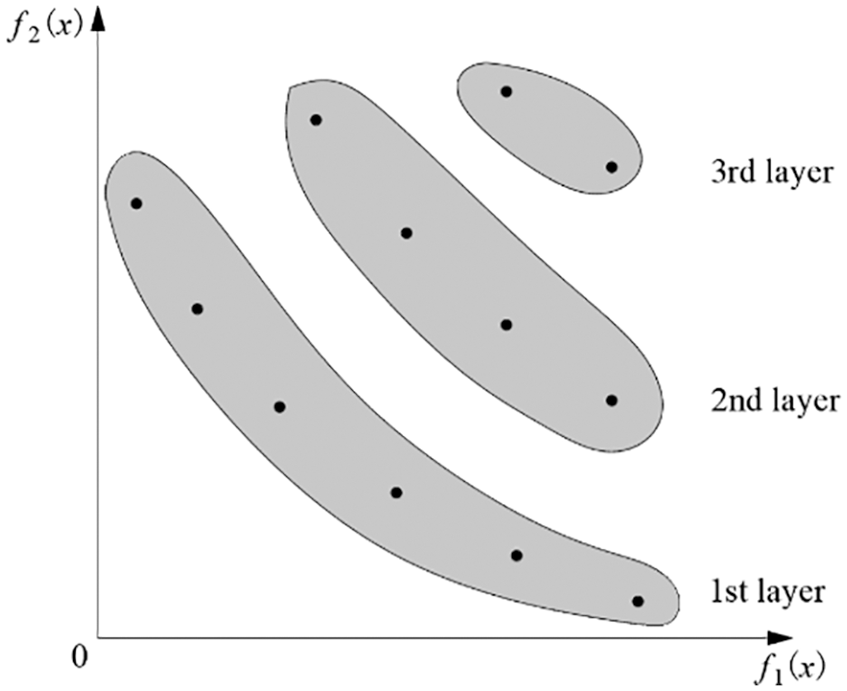
Figure 4: The pareto set. The vectors in each layer make up the pareto front

In the same layer, the mass of solutions is compared by crowding distance to increase population diversity. The crowding distance of one point is defined as the sum of the objective function value of adjacent solutions in each dimension.

The offspring population can be obtained by performing crossover and mutation on the parent population. Mix the offspring population and the parent population. The following elite retention strategy was adopted to select individuals to keep the population size at N (N denotes the population size): Make a non-dominant order for the mixed-population, then put them into the next generation from the 1st layer. If all individuals in one layer cannot be completely put into the next generation, put them into the next generation in order of the crowding distance until the next generation contains N individuals. The complete process of the NSGA-Ⅱ algorithm is shown in Fig. 5.

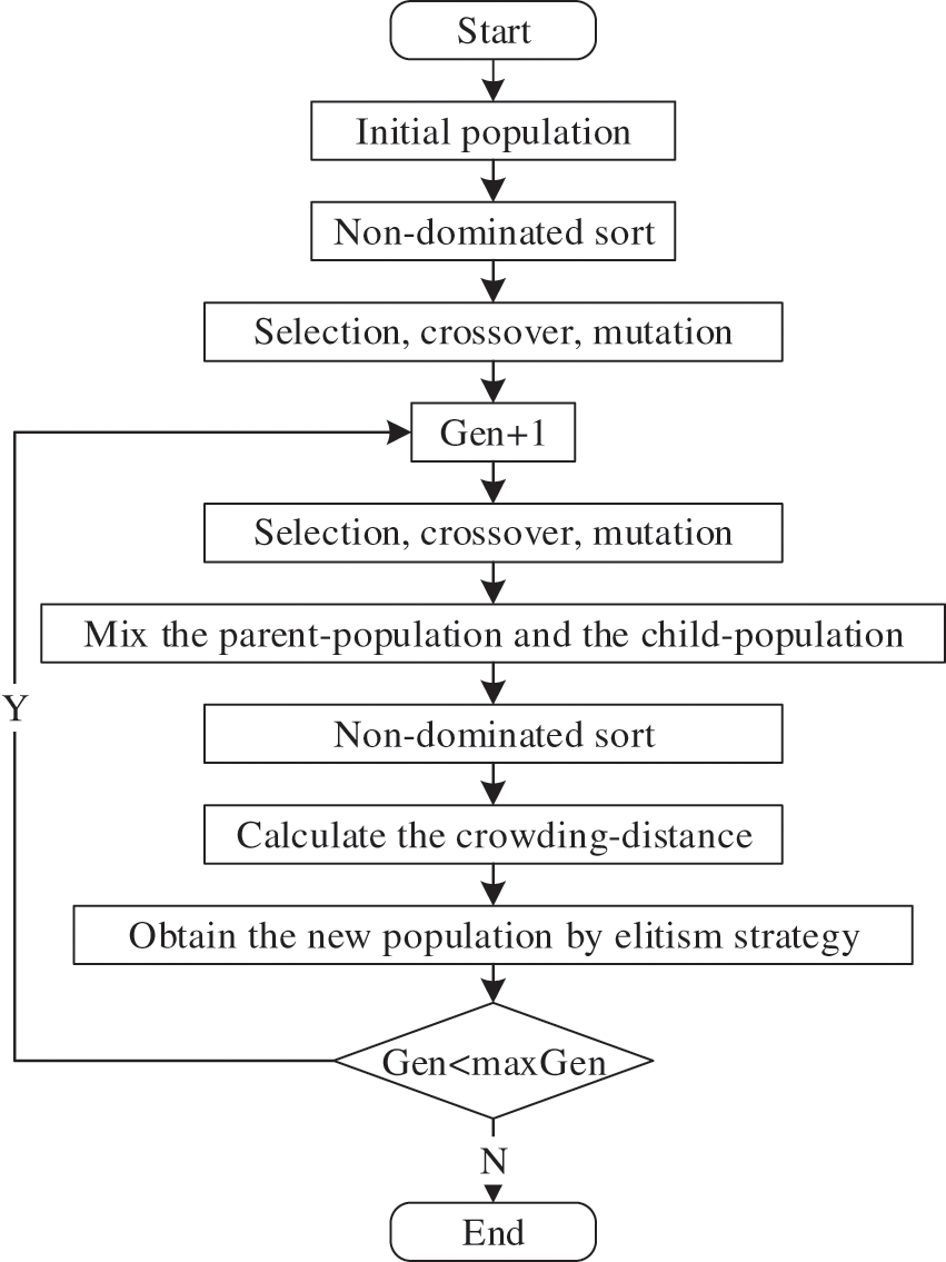
Figure 5: Flowchart of NSGA-Ⅱ II algorithm

4.2 Differential Evolution Algorithm

The NSGA-Ⅱ algorithm provides a solution for multi-objective optimization. However, due to the high dimensionality caused by too many path points, the convergence rate may be slow. When compared to other evolutionary algorithms for high-dimensional optimization, the DE algorithm has a faster convergence rate, fewer control parameters, and lower space complexity [18].

The individual Xi,g in the parent population in the DE algorithm is called the target individual. Three different individuals in the current population get the mutant individual Vi,g corresponding to Xi,g through the mutation operation as Eq. (25)

Vi,g=Xr1,g+F⋅(Xr2,g−Xr3,g)(25)

where the r1,r2,r3∈[1,N] and r1≠r2≠r3=i, F∈(0,1).

Binomial crossover is usually used as the crossover operation of the DE algorithm, which can be expressed as Eq. (26)

Ui,gj={Vi,gjif(randij(0,1)≤CRorj=jrand)Xi,gjotherwise(26)

where CR∈(0,1), jrand is an integer and jrand∈[1,D], D denotes the dimensions of Xi,g. Ui,gj denotes the individual of child-population corresponding to Xi,g.

4.3 Redundancy Optimization Algorithm

In the redundancy optimization of robot milling, the dimensionality of optimization is determined by the number of points in the path. Too many points result in high dimensionality, which will lead to high complexity, heavy computational burden, and low convergence rate.

Combine the NSGA-II and DE algorithms to fully utilize the benefits of both algorithms. Using the DE algorithm’s crossover and mutation operations in the NSGA-II method, an improved method for solving multi-objective optimization problems with high convergence rate and low complexity was proposed.

Due to the number of path points being uncertain in actual production, changing the number of points will result in a change in optimization dimensionality. Different optimization dimensions have different requirements on algorithm parameters, and the calculation time is also different. To make the optimization algorithm more universal, the path is segmented as shown in Fig. 6. Then the segments can be optimized one by one to ensure the same dimensionality of each optimization.

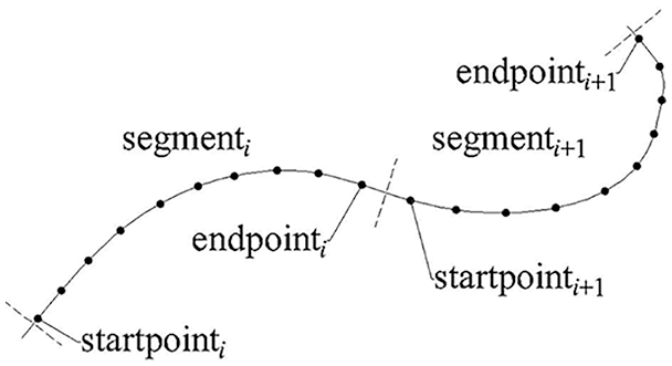
Figure 6: Schematic diagram of path segmentation

The number of points p in each segment of the path can be reasonably determined based on the computer’s computing performance. As shown in Fig. 6, the segmenti presents the ith segment in a path. The startpointi and endpointi present the first point and the last point in segmenti respectively. If the number of points contained in the path is not an integer multiple of p, the number of points in the path needs to be supplemented. The path can be supplemented by copying the last point of the path. Besides, the supplementary points do not affect the result of the optimization algorithm because they are coincident. To ensure the smoothness between adjacent segments, the velocity of endpointi needs to participate in the calculation of the acceleration of startpointi+1. Adjust Eqs. (4) and (5) to Eqs. (27) and (28)

kwji={kθji−kθji−1△ti+△ti+1(kθji−kθji−1)−△ti(kθji+1−kθji)△ti+1(△ti+1+△ti)i∈(1,N−1]kθji−k−1θjN△ti+△ti+1(kθji−k−1θjN)−△ti(kθji+1−kθji)△ti+1(△ti+1+△ti)i=1,k∈(1,S]0i=N0i=1,k=1(27)

kaji={2ti+1(kθji−kθji−1)−ti(kθji+1−kθji)titi+1(ti+ti+1)i∈(1,N−1]2ti+1(kθji−k−1θjN)−ti(kθji+1−kθji)titi+1(ti+ti+1)i=1,k∈(1,S]0i=N0i=1,k=1(28)

where the kwji, kθji, kaji denotes the angular velocity, the angular variable, and the angular acceleration of jth joint at the ith point respectively in the kth segment, and the N, S denotes the number of points in one segment and the number of segments in one milling path.

Fig. 7 depicts the optimization algorithm’s process. Once the milling path is given, the path will be divided into several segments. Each segment is then sequentially optimized individually. Perform the normalization and real-coded operation on the redundancy DOF of each point in the segment, then the optimization variable vector [γ1,γ2,…,γN] is obtained. After initialization, crossover and mutation operation are performed on the population according to Eqs. (25) and (26). According to Section 4.2, we get a set of optimal solutions (Pareto front) for each segment. For the first segment, choose the solution which can make the distance between the startpoint1 and the initial position short, this can be expressed as Eq. (29)

minp∈{1,2,…,P}⁡{∑j=16|qstartpoint1p,j−qinitialpositionp,j|}(29)

where the P denotes the number of solutions contained in the Pareto front, and the qstartpoint1p,j denotes the angular of the jth joint at the startpoint1 in the pth solution.

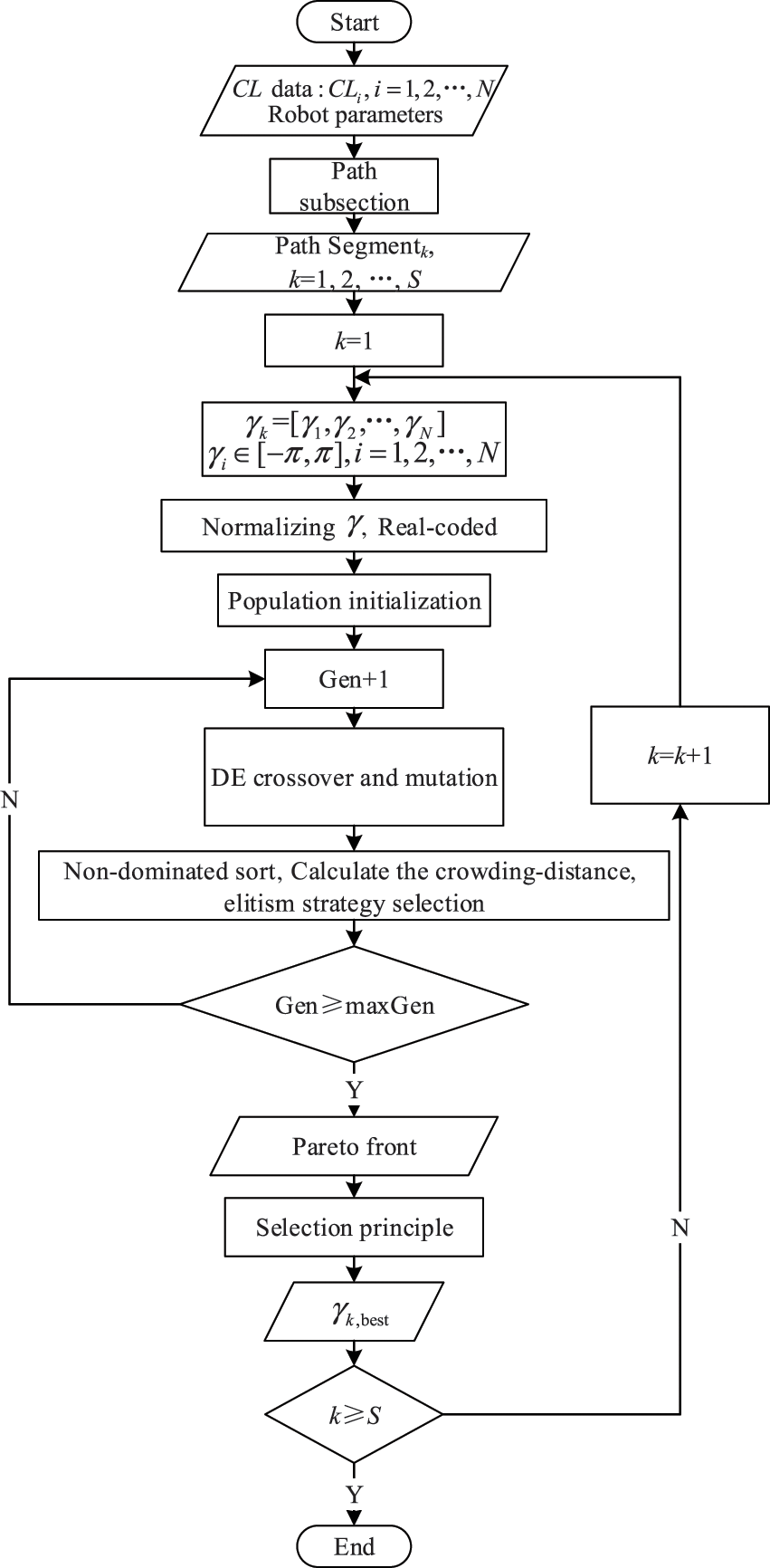
Figure 7: Flow chart of the algorithm for redundancy optimization

For the other segments, choose the solution from the Pareto front according to Eq. (30)

minp∈{1,2,…,P}⁡{∑j=16|qstartpointip,j−qendpointi−1p,j|}(30)

This selection principle can further avoid the discontinuity at the junction of each segment caused by the path segmentation.

5  Simulations

In this section, the proposed method was used to optimize the redundancy of the milling path generated by the UG processing module, and the optimization results were simulated using the ABB RobotStudio to validate the method’s effectiveness.

5.1 Simulation for Different Milling Paths

As illustrated in Fig. 8, the ABB IRB-1600 robot was chosen to build the milling system, its D-H parameter is depicted in Table 1. Fig. 9 shows the 100 points milling path and 300 points milling path generated by the commercial CAM software UG NX.

Figure 8: The robot milling system built by ABB IRB-1600

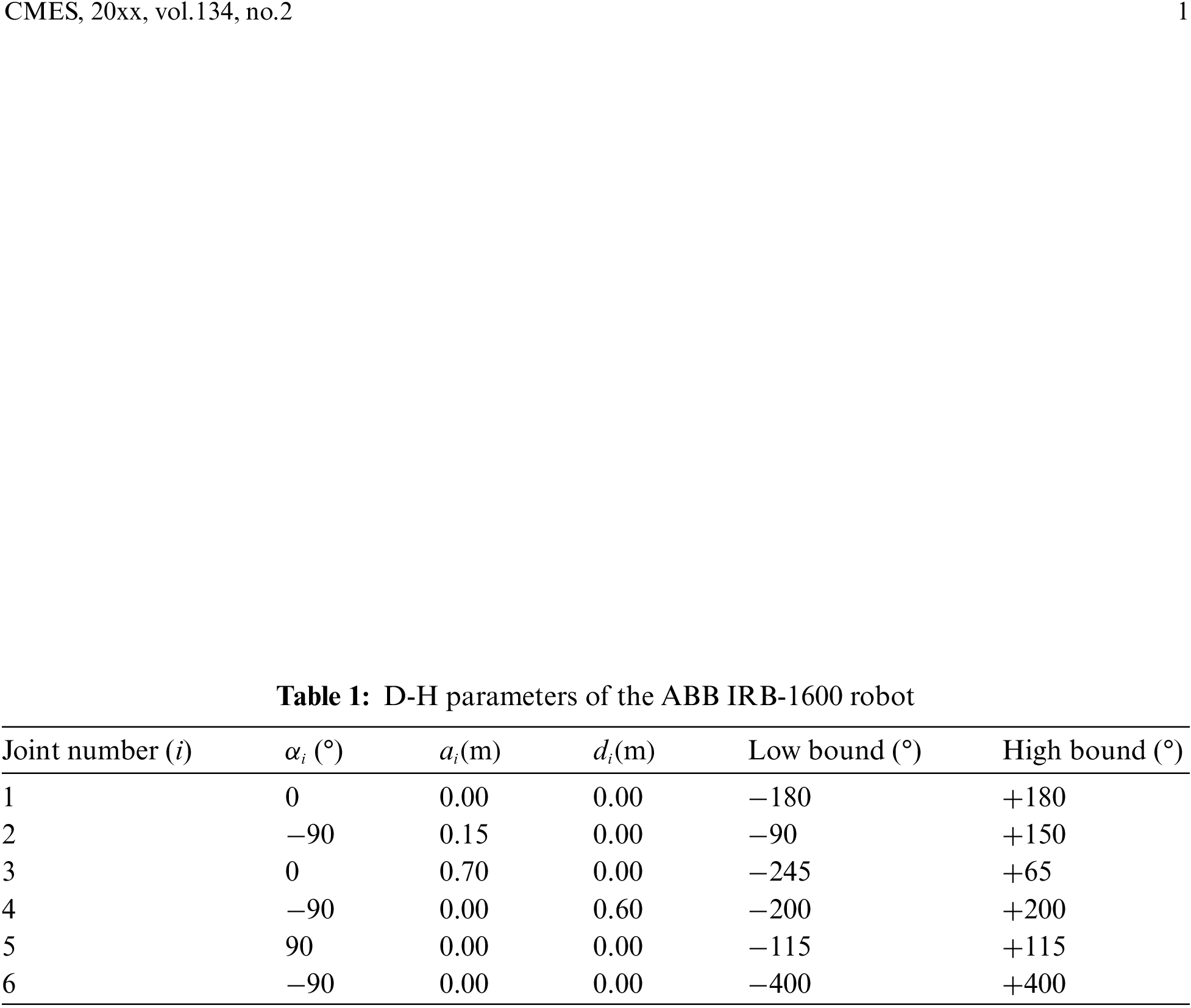
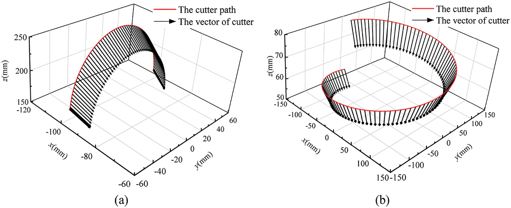
Figure 9: The cutter location of the milling path for simulation. (a) The cutter location of the 100-points path. (b) The cutter location of the 300-points path

The optimization results were substituted into Eq. (23) to get the joint vector of each point. The joint vector was established as the joint target and path by RobotStudio. The signal analyzer in the ABB RobotStudio simulation module can obtain instantaneous joint angles at each point in the path. Figs. 10a and 10b indicate the joint angle of each joint in the path while machining. It can be seen from Fig. 10 that the motion of each joint is smooth except for the fluctuation around 235 s in Fig. 10b. The singularity factors k1 = 0.07586 and k2 = 0.0167 are closed to 0 at 235.3 s. Approaching constraint is the main reason for the fluctuation in the curve of the joint angles around 235 s. However, as shown in Fig. 11b and Table 2, the joint velocity at 235.3 s is still far below the maximum speed that the robot can reach. So we can say that this path is “relatively smooth” and its fluctuation does not have a great influence on the machining quality.

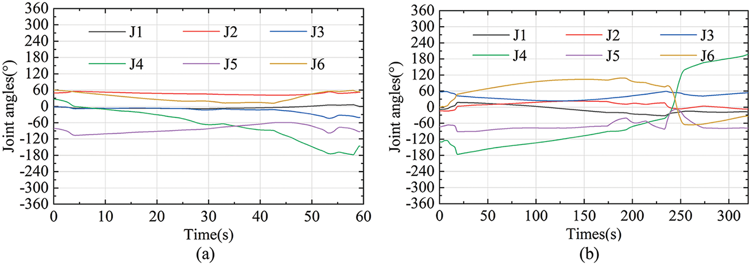
Figure 10: The joint angles along the milling path. (a) The joint angles along the 100-points path. (b) The joint angles along the 300-points path

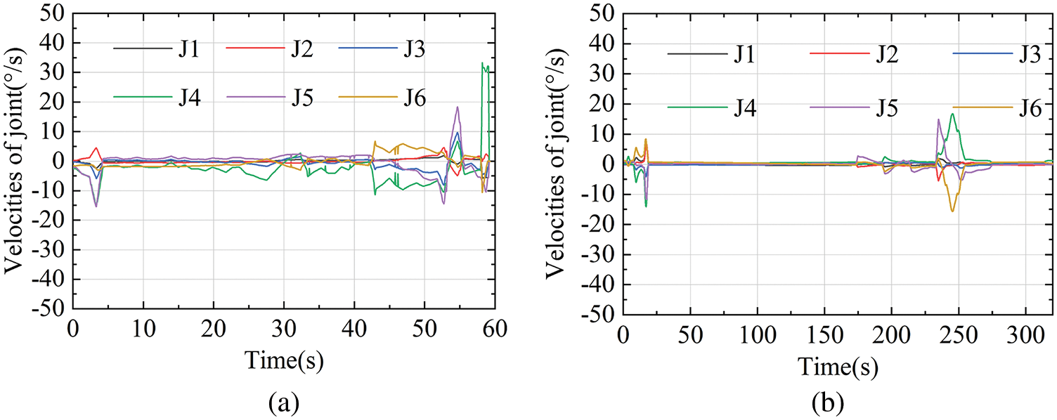
Figure 11: The joint velocities along the milling path. (a) The joint velocities along the 100-points path. (b) The joint velocities along the 300-points path

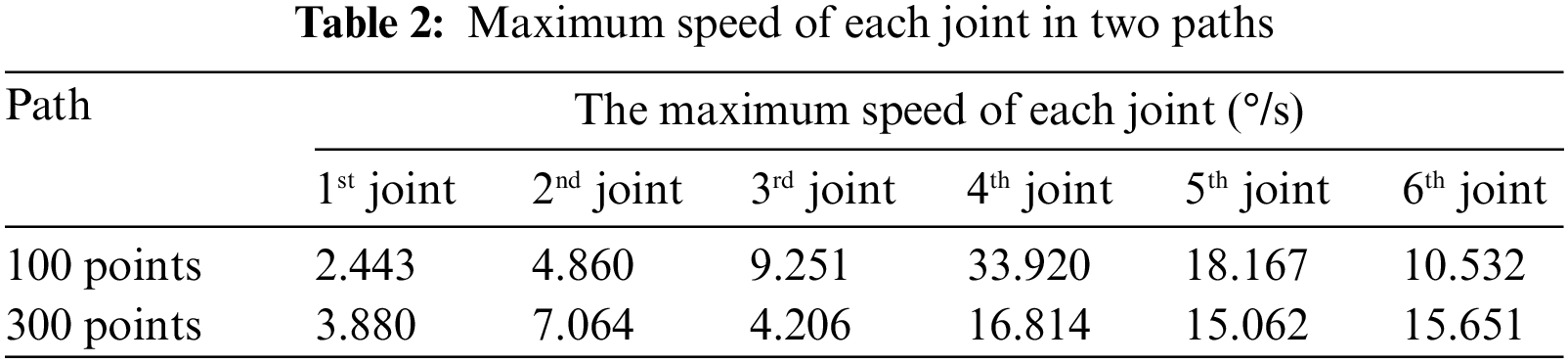
Figs. 11a and 11b display the velocity of each joint The maximum speed is shown in Table 2. According to Table 2, the maximum machining speed of each joint is substantially lower than the maximum speed that the robot can be achieved. As shown in Figs. 12a and 12b, the accelerations of the two paths only fluctuate in a few places. And the main reason for the several abrupt changes in velocity and acceleration is the large jumps in the trajectory planned by UG or the joints are close to the robot limits. The total motor energy of the two paths is depicted in Fig. 13.

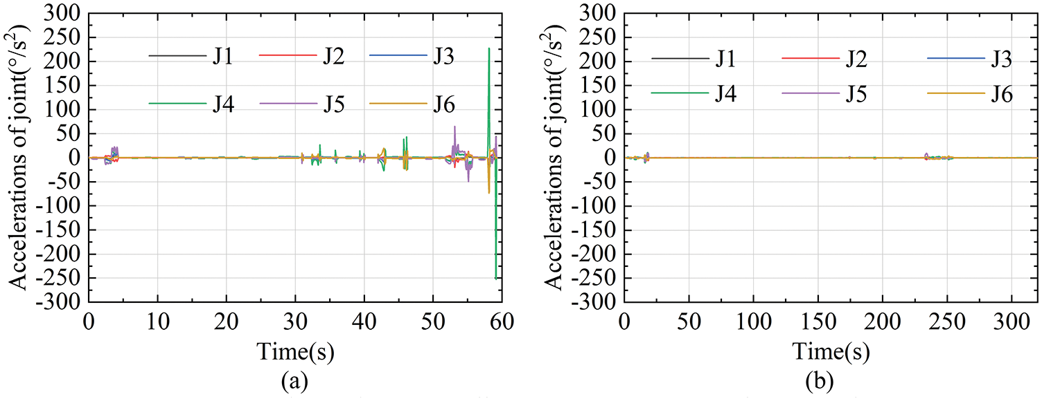
Figure 12: The joint accelerations along the milling path. (a) The joint accelerations along the 100-points path. (b) The joint accelerations along the 300-points path

Figure 13: The total motor energy of two paths. (a) The total motor energy of the 100-points path. (b) The total motor energy of the 300-points path

Bruno Siciliano proposed the manipulability measure to quantify the distance between robot pose and singularity [14]. This method is widely used in robot singularity avoidance. In this paper, the manipulability measure is used to prove the validity of the singularity constraint. The formula for the manipulability measure can be expressed as Eq. (31)

ω(q)=|det(J(q))|(31)

where the det(J(q)) denotes the determinant of the Jacobi matrix. To make it more intuitive, we plotted the ratio of ω(q) to the maximum ω(q) in Fig. 14, it can be calculated as Eq. (32)

κ(q)=ω(q)ωmax(q)(32)

Figure 14: The κ(q) at each cutter location. (a) The κ(q) of the 100-points path. (b) The κ(q) of the 300-points milling path

The smaller κ(q) is, the closer the robot is to the singularity. When the robot reaches the singularity, κ(q)=0. The ωmax(q) of IRB1600 robot was obtained as 0.4806 by the fminsearch function. As shown in Fig. 14, there is κ(q)>0 at any point on the curve. Thus the constraint based on the singularity factors is valid. However, κ(q) cannot be maximized since the singular factors only exist as a constraint of the algorithm in this paper.

5.2 Simulation for Different Optimization Methods

In this section, the proposed method is compared with the graph-based method [7] to prove the superiority of this algorithm.

The essential idea of the graph-based method, as illustrated in Fig. 15, is to disseminate the possible solution of redundancy optimization, and use the points of each column to signify the solution of the corresponding CLi. The length of the connecting line between any two points in two adjacent columns is expressed by weight. The goal of this method is to search a path with the minimum weight in the whole search space.

Figure 15: The search space of the graph-based method

The path to be optimized is displayed in Fig. 16. Set the optimization parameters Cr = 0.4, F = 0.85 in the proposed algorithm. The joint angle in the path while machining of two methods is shown in Fig. 17. It can be noticed that the curves of the 4th joint are the least smooth of the two algorithms’ outcomes.

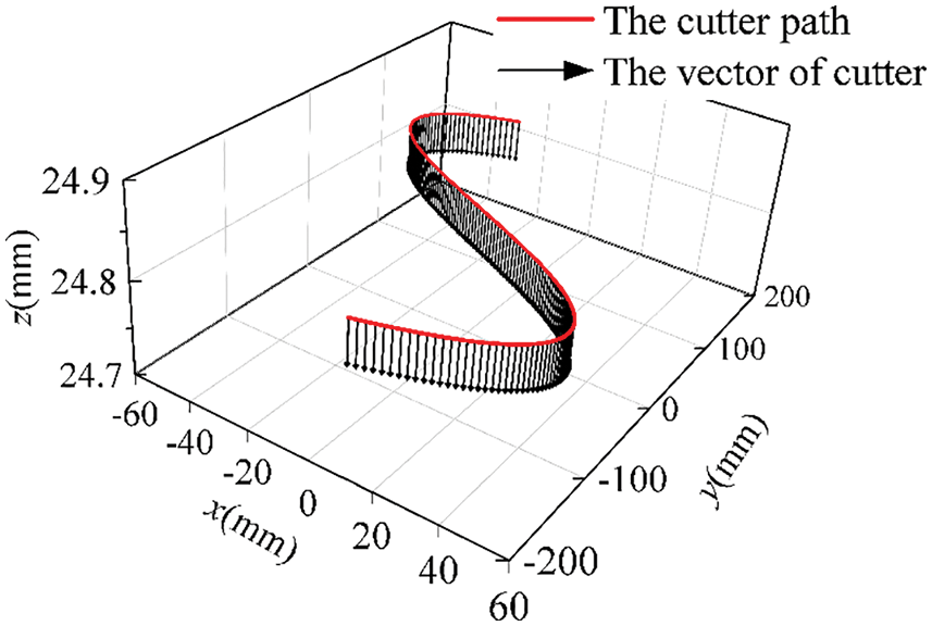
Figure 16: The milling path of the simulation for the different optimization methods

Figure 17: The joint angles along the path of the simulation for comparison of (a) the proposed method and (b) the comparison method

Fig. 18 shows the calculated acceleration of the 4th joint optimized by the two methods. It is clear that, when compared to the comparison method, the presented method offers significant advantages in terms of acceleration. The main reason is that the number of values of γ in the comparison algorithm is limited. The comparison algorithm can only find the optimal solution among finite solutions, which is similar to the local optimal solution. In addition, increasing the number of γ will lead to the heavy computational burden, which is the disadvantage of the ergodic algorithm compared with the real number coding in the heuristic optimization algorithm. Table 3 shows the absolute maximum acceleration of each joint optimized by the two algorithms. When compared to the comparison method, it can be shown that the suggested algorithm’s maximum acceleration is small.

Figure 18: The calculated acceleration of the 4th joint optimized by two the methods

The ABB RobotSudio signal analyzer also records the total motor energy of the robot as it moves. The total motor energy of the path generated by the two methods is shown in Fig. 19. The total motor energy of the path generated by the proposed method is 44.2% less than the one generated by the method for comparison. Due to the smaller joint velocity fluctuation, the fluctuation of the feedrate of TCP milling is also smaller, which results in a shorter machining time of the path. The machining time of the path generated by the proposed method is 78.11 s while the other one generated by the comparison method is 83.11 s.

Figure 19: The total motor energy of the path generated by the two methods

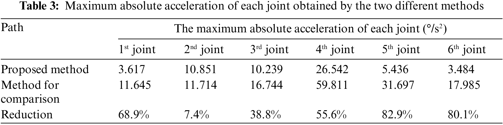
It is easy to conclude that the proposed algorithm not only consumes less energy than the comparison algorithm but also consumes less time. In addition, as depicted in Fig. 18 and Table 3, the path generated by the proposed algorithm has better smoothness than that generated by the comparison algorithm. Therefore, the method proposed in this paper achieves better manufacturing quality than the comparison method.

This algorithm for comparison is essentially a traversal algorithm, whose optimization quality has a great relationship with sampling step length and sampling quantity. Smaller sampling step length and larger sampling quantity will result in better optimization quality but a heavy computational burden. In this paper, the two optimization methods were run on the same computer. The computation time of the graph-based method and the proposed method were 36.9 and 30.7 s, respectively.

From the above simulation results, it can be seen that the algorithm proposed in this paper can effectively solve the problem of milling robot redundancy. It can be concluded from Section 5.1 that the algorithm is not affected by the number of CL in the path, and the quality of the solution does not decrease with the increase of the number of CL. And compared with other algorithms in Section 5.2, the algorithm proposed in this paper also improves the quality of the solution.

6  Conclusion

In this paper, a new optimization method is put forward to optimize the redundant DOF of milling robot in shipbuilding. This method combines NSGA-Ⅱ and DE algorithms to optimize the milling path of the robot with multiple objectives. A piecewise method is proposed to protect the optimization algorithm’s calculation efficiency from the effect of the number of path points. The simulation results show that the proposed method is efficient for multi-objective redundancy optimization in robot milling applications to improve the path smoothness and reduce the robot energy consumption. This method offers a novel solution to the problem of robot milling redundancy, and it has a wide range of applications in shipbuilding machining.

Acknowledgement: The authors are responsible for the contents of this publication. Besides, the authors would like to thank lab classmates for contribution to the writing quality.

Funding Statement: The authors received no specific funding for this study.

Conflicts of Interest: The authors declare that they have no conflicts of interest to report regarding the present study.

References

1. Ruiz, A. G., Santos, J. C., Croes, J., Desmet, W., Maira, M. S. (2018). On redundancy resolution and energy consumption of kinematically redundant planar parallel manipulators. Robotica, 36(6), 809–821. DOI 10.1017/S026357471800005X. [Google Scholar] [CrossRef]
2. Zhang, Y. N., Ma, S. G. (2007). Minimum-energy redundancy resolution of robot manipulators unified by quadratic programming and its online solution. IEEE International Conference on Mechatronics and Automation, vol. 1–5, Harbin, China. [Google Scholar]
3. Peng, J. F., Ding, Y., Zhang, G., Ding, H. (2020). Smoothness-oriented path optimization for robotic milling processes. Science China-Technological Sciences, 63(9), 1751–1763. DOI 10.1007/s11431-019-1529-x. [Google Scholar] [CrossRef]
4. Zhang, Y., Ge, S. S., Lee, T. H. (2004). A unified quadratic-programming-based dynamical system approach to joint torque optimization of physically constrained redundant manipulators. IEEE Transactions on Systems Man and Cybernetics Part B-Cybernetics, 34(5), 2126–2132. DOI 10.1109/TSMCB.2004.830347. [Google Scholar] [CrossRef]
5. Al Khudir, K., de Luca, A. (2018). Faster motion on cartesian paths exploiting robot redundancy at the acceleration level. IEEE Robotics and Automation Letters, 3(4), 3553–3560. DOI 10.1109/LRA.2018.2853806. [Google Scholar] [CrossRef]
6. Boscariol, P., Richiedei, D. (2019). Trajectory design for energy savings in redundant robotic cells dagger. Robotics, 8(1), 15. DOI 10.3390/robotics8010015. [Google Scholar] [CrossRef]
7. Dolgui, A., Pashkevich, A. (2009). Manipulator motion planning for high-speed robotic laser cutting. International Journal of Production Research, 47(20), 5691–5715. DOI 10.1080/00207540802070967. [Google Scholar] [CrossRef]
8. Doan, N. C. N., Tao, P. Y., Lin, W. (2016). Optimal redundancy resolution for robotic arc welding using modified particle swarm optimization. 2016 IEEE International Conference on Advanced Intelligent Mechatronics (AIM), pp. 554–559. Banff, Canada. [Google Scholar]
9. Yeasmin, S., Shill, P. C., Paul, A. K. (2017). A new method for smooth trajectory planning for 3R robot arm using enhanced particle swarm optimization algorithm. 3rd International Conference on Electrical Information and Communication Technology, pp. 1–6. Khulna, Bangladesh. [Google Scholar]
10. Machmudah, A., Parman, S., Baharom, M. B. (2018). Continuous path planning of kinematically redundant manipulator using particle swarm optimization. International Journal of Advanced Computer Science and Applications, 9(3), 207–217. DOI 10.14569/issn.2156-5570. [Google Scholar] [CrossRef]
11. Shibata, T., Abe, T., Tanie, K., Nose, M. (1997). Motion planning by genetic algorithms for a redundant manipulator using a model of criteria of skilled operators. Information Sciences, 102(1–4), 171–186. DOI 10.1016/S0020-0255(97)00049-2. [Google Scholar] [CrossRef]
12. Ma, J. W., Liu, Y., Zang, S. F., Wang, L. (2020). Robot path planning based on genetic algorithm fused with continuous bezier optimization. Computational Intelligence and Neuroscience, 2020, 1–10. DOI 10.1155/2020/9813040. [Google Scholar] [CrossRef]
13. Wiedmeyer, W., Altoe, P., Auberle, J., Ledermann, C., Kroger, T. (2021). A real-time-capable closed-form multi-objective redundancy resolution scheme for seven-DoF serial manipulators. IEEE Robotics and Automation Letters, 6(2), 431–438. DOI 10.1109/LSP.2016.. [Google Scholar] [CrossRef]
14. Siciliano, B., Sciavicco, L., Villani, L., Oriolo, G. (2010). Robotics: Modelling, planning and control. USA: Springer Publishing Company. [Google Scholar]
15. Gautschi, W. (2012). Numerical analysis. Boston: Birkhäuser. [Google Scholar]
16. Xiao, W., Ji, H. (2012). Redundancy and optimization of a 6R robot for five-axis milling applications: Singularity, joint limits and collision. Production Engineering, 6(3), 287–296. DOI 10.1007/s11740-012-0362-1. [Google Scholar] [CrossRef]
17. Deb, K., Pratap, A., Agarwal, S., Meyarivan, T. (2002). A fast and elitist multiobjective genetic algorithm: NSGA-II. IEEE Transactions on Evolutionary Computation, 6(2), 182–197. DOI 10.1109/4235.996017. [Google Scholar] [CrossRef]
18. Rainer, S., Kenneth, P. (1997). Differential evolution–A simple and efficient heuristic for global optimization over continuous spaces. Journal of Global Optimization, 11(4), 341–359. DOI 10.1023/A:1008202821328. [Google Scholar] [CrossRef]
Cite This Article
Copyright © 2023 The Author(s). Published by Tech Science Press.
This work is licensed under a Creative Commons Attribution 4.0 International License , which permits unrestricted use, distribution, and reproduction in any medium, provided the original work is properly cited.
Downloads
Citation Tools