
 Submit a Paper
 Propose a Special lssue
 Open Access
ARTICLE
A Consistent Time Level Implementation Preserving Second-Order Time Accuracy via a Framework of Unified Time Integrators in the Discrete Element Approach
1 School of Energy and Power Engineering, Nanjing University of Science and Technology, Nanjing, 210094, China
2 Department of Mechanical Engineering, University of Minnesota-Twin Cities, Minneapolis, 55455, USA
* Corresponding Authors: Kumar Tamma. Email: ; Xiaobing Zhang. Email:
Computer Modeling in Engineering & Sciences 2023, 134(3), 1469-1487. https://doi.org/10.32604/cmes.2022.021616
Received 24 January 2022; Accepted 21 April 2022; Issue published 20 September 2022
 View Full Text
 Download PDF
Abstract
In this work, a consistent and physically accurate implementation of the general framework of unified second-order time accurate integrators via the well-known GSSSS framework in the Discrete Element Method is presented. The improved tangential displacement evaluation in the present implementation of the discrete element method has been derived and implemented to preserve the consistency of the correct time level evaluation during the time integration process in calculating the algorithmic tangential displacement. Several numerical examples have been used to validate the proposed tangential displacement evaluation; this is in contrast to past practices which only seem to attain the first-order time accuracy due to inconsistent time level implementation with different algorithms for normal and tangential directions. The comparisons with the existing implementation and the superiority of the proposed implementation are given in terms of the convergence rate with improved numerical accuracy in time. Moreover, several schemes via the unified second-order time integrators within the framework of the GSSSS family have been carried out based on the proposed correct implementation. All the numerical results demonstrate that using the existing state-of-the-art implementation reduces the time accuracy to be first-order accurate in time, while the proposed implementation preserves the correct time accuracy to yield second-order.Keywords
In order to numerically describe the behavior of granular materials (not continuous body) represented as a collection of large number of distinct particles, the discrete/distinct element method (DEM), proposed in [1], is being widely used for its ease of implementation and versatility. In the DEM technique, each particle element can undergo large displacement and rotation, and the deformations of individual particle elements are assumed to be small, compared with their displacements; hence we can treat the elements as rigid bodies and the deformation is usually described in terms of the relative normal displacement and the relative tangential displacement between the particles in contact. Consequently, the evaluation of those two displacements has a significant influence on both the dynamic response of particles and the numerical accuracy of the simulation.
One of the common applications for the DEM is particle packing. Various packing methods using DEM have been studied previously such as, Formation of a pile, i.e., sand piling process [2–6], pouring or depositing particles under gravity [7–12]. The DEM particle packing is also used in pharmaceutical field for powder tableting [13,14]. Another field of application using DEM is simulating particle flow; and a commonly studied example is ball mill mixer simulation; some of which include, horizontally rotating drums [15–18], tumbling ball mill [19–21]. Drum and mill are commonly used in industries for mixing, drying or coating subjects; thus, there is extensive interest among researchers in this study. Besides, the DEM is still studied and utilized in recent studies such as solid-liquid flow simulation [22], impact disruption of cohesive soft sphere simulation [23], granular shear flows of dry flexible fibers [24] and non-spherical complex granular simulation [25].
Furthermore, the DEM not only simulates granular flow, but it can also be used for solid body analysis and assessing fracture as studied in [26]. Recently, the DEM has been expanded to be able to solve multi-physics applications where granular particles interact with a continuous body, be it structural or thermodynamics. An Extended Discrete Element Method (XDEM) has been proposed in [27] which couples continuous body analysis method and DEM together without losing small scale information from commonly used volume averaging concept. The XDEM allows those microscale information from particles to accurately influence a macroscopic body. The XDEM opens up a wide variety of possible physical applications in many fields of study.
In transient dynamic simulation of the DEM type problems, contact forces and particle motion need to be evaluated and updated at every time step. The widely used time integrations in the DEM numerical simulations include the explicit Euler method, fourth-order Runge-Kutta (RK-4) method, and central difference method/velocity verlet method, etc. It is straightforward to implement these methods in the DEM simulation; however, these explicit time stepping techniques possess several numerical disadvantages in addition to the conditionally stable features; for example, the Euler methods are first-order accurate in time, RK-4 method requires additional computations of high-order derivatives of differential variables [28,29], and the central difference method is a non-dissipative scheme, i.e., it cannot introduce numerical dissipation if one needs to. Also, past practices poorly model the tangential physics of particle interactions. Recently, a unified time integration framework, under the umbrella of the so-called generalized single-step single-solve (GSSSS) family of algorithms, including not only implicit, but also explicit single-step single-solve algorithms, which can also be written in a linear three-step form, has been proposed in [30]. This single simulation tool kit, which has been originally developed in the field of computational structural dynamics, encompasses not only most existing algorithms that are second-order time accurate and are commonly used over the past 50 years or so, but it additionally inherits a wide variety of new implicit and explicit time integration schemes also with second-order time accuracy, including the explicit central difference method as a special case. To implement these time integrations in DEM and preserve the numerical accuracy of the algorithms, the contact force is required to be evaluated in a consistent way with the selected time integrations in both normal and tangential directions. According to our knowledge, most of the existing literature have been embedding the first-order accurate updating evaluation of tangential displacement into the first/second-order accurate time integrations. The specifics are shown in Section 2, leading to reduced accuracy.
In this work, the main objective is to show the consistent implementation of the GSSSS family of algorithms to the simulation of granular assemblies with DEM while retaining all the advantages of numerous methods within the present framework of algorithms. It is worthy to mention that one major drawback of the DEM technique, as well as the other particle based methods or meshless methods [31–35], is contact detection or neighboring particle search. To circumvent this issue, the linked list is employed to detect the contacting neighbor particles. In addition, Open Multi-Processor (Open MP) is implemented to reduce the simulation computational time. The outline of the rest of the paper is as follows. Section 2 presents the basic theory of DEM formulations and both the linear and the nonlinear model of contact forces and torques are presented in detail. The GSSSS unified time integrators are highlighted in Subsection 2.2 and the specifics of the proposed consistent tangential displacement evaluation is derived and compared with the existing tangential displacement evaluation technique carefully. The effectiveness of the proposed consistent tangential displacement evaluation is demonstrated and illustrated using simple numerical examples in Section 3. Finally, the conclusions are drawn and presented in Section 4. This study shows that the DEM with explicit schemes within the GSSSS family of algorithms achieves and consistently preserves second-order time accuracy; the consistent time level implementation and preserving the second-order time accuracy for the presented results for a wide variety of time integrators in the present unified framework include features such as no overshoot in displacement or no overshoot in velocity or no overshoot in both displacement and velocity for a given set of initial conditions of the particles and differs from algorithm to algorithm.
2 Discrete Element Method with the Explicit GSSSS Family of Algorithms
DEM is a numerical simulation technique for a system of small “distinct” particles/elements, such as powders and granular materials. For the sake of simplicity, we assume the shape of every particle/element in a system is a disk in the two-dimensional Euclidean space
Let
where
where
the projection of
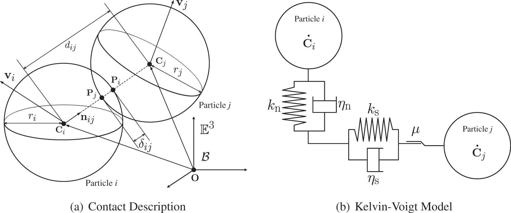
Figure 1: (a) Pictorial illustration of particles i and j in contact; and (b) the Kelvin-Voigt model for particles i and j in contact.
Note that
Hence,
Similarly, we can derive the relative acceleration vectors of point
where
respectively.
Contact Forces and Torques
The resultant contact force and torque acting on particle i are defined as the summations of the contact forces and torques, respectively, acting on particle i from all particles
Linear Model: The contact force acting on particle i from particle j can be uniquely decomposed into the contact forces in the normal direction (
where
The viscous damping coefficient
Similarly, the tangential contact force,
where
We usually take
Nonlinear Model: There exist several nonlinear models developed for DEM in the literature to obtain more accurate, realistic simulation results. A common nonlinear model of DEM, proposed in [37], is based on the classical Hertzian contact theory and Mindlin theory [38,39]. The normal contact force,
However, as opposed to the linear model,
with
On the other hand, the tangential contact force,
with
where
2.2 Transient Analysis: A Consistent Time Level Implementation of Unified Time Integrators
Applying the Newton-Euler equation to particle i for
where
In a unified format for all particles (
Time Discretization
Consider the temporal discretization of the governing equations for a time interval
where the algorithmic acceleration, velocity, and configuration vectors are defined as
respectively, for
The algorithmic parameters, also known as the DNA [discrete numerically assigned] markers, are defined with the input scalar algorithmic parameters
for the U0(
for the V0(
Algorithmic Evaluation of
Suppose particles i and j are in contact during a time interval
where
where
Note that
where
Remark
1. If the contact starts at time
2. When
3. When slip occurs at the algorithmic time level
4. The evaluations of
It is worth noting that the tangential acceleration is usually not included during the computations of the tangential contact forces, i.e., for the central difference method, for example,
is inconsistently used instead of Eq. (33) of the most literature; in this case, the order of accuracy of a scheme within the algorithmic framework presented reduces to only one.
5. For the evaluation of the tangential displacement
3 Numerical Experiments and Discussion
To verify and validate the concepts described in the previous section, two numerical experiments are given in this section. The main objective of Section 3.1 is to compare the numerical results by traditional tangential displacement evaluation and the proposed consistent evaluation method employing the Central Difference Method. It is worth noting that Central Difference Method is the most widely used explicit second-order time accurate integrator in solving dynamic problems. Therefore, we simply use it as the benchmark in the following simulations. The accuracy in time with different tangential displacement evaluations are given as well. In Section 3.2, a simple 3D granular cube falling problem is simulated with several selected second-order time accurate schemes from the GSSSS unified time integrators. The numerical performances of different schemes with different tangential displacement evaluations are discussed. The linked list algorithm is used to improve the particle searching process and parallel computing is also used in this work. In addition, the calculation time for the 3D case is provided to demonstrate the computational efficiency of the proposed method.
To valid our proposed approach and the DEM code, two cases are designed to test the performance of the proposed tangential displacement evolution. Case I is designed to extract the tangential displacement calculation in the general discrete element method. The influence of normal direction is avoided in Case I via fixing a two dimensional disk with only initial angular velocity and constant normal force. Case II gives a general ball falling problem with gravity and the comparisons of traditional and consistent tangential displacement evolution.
Case I: The equation of the tangential motion can be derived to yield a second-order ODE (ordinary differential equation) from Eq. (17), which has an analytical solution for the linear equation. To test our new proposed tangential displacement evaluation method, a very simple and specific physical problem is designed as a 2-D disk with fixed translational movement. As illustrated in Fig. 2 (left), although the normal force is involved, the tangential movement can be easily extracted. The disk is fixed at the origin
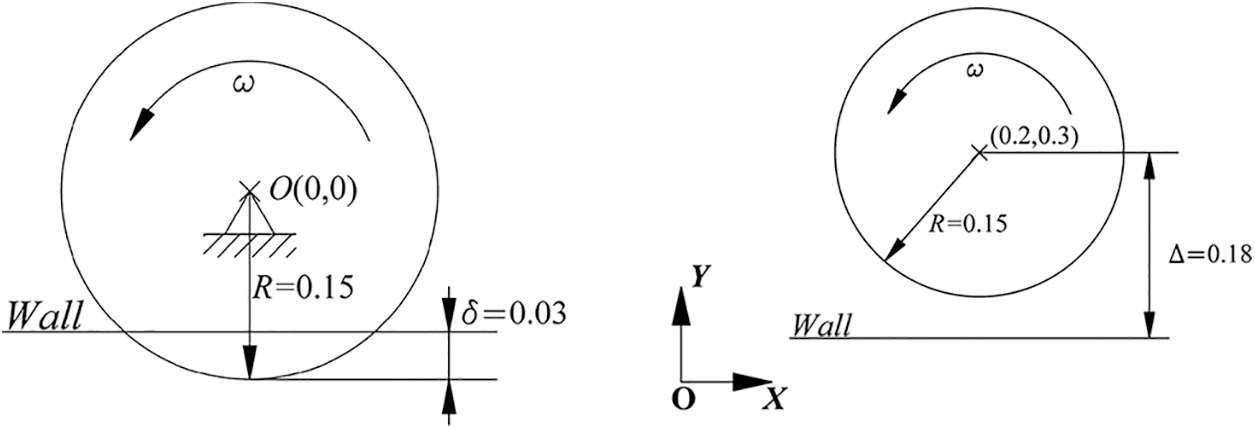
Figure 2: Schematic of the problem. Left: Case I and right: Case II
The comparison of the results with different tangential displacement evaluation methods is given in Fig. 3. Both the proposed consistent time level method and the traditional method show good agreement with the analytical solutions in angular position, velocity and acceleration. In this part, our interest is to simply show that the proposed method has the improved or same performance as the traditional method in the sense of capturing physical phenomena.
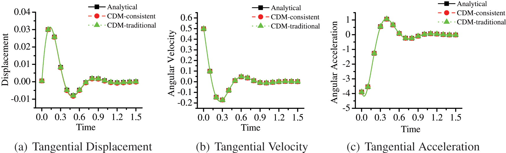
Figure 3: The time history of tangential motion with different tangential displacement evaluation methods
Case II: To complete the validation of our code, a general single ball falling problem shown in Fig. 2 (right), is simulated by different tangential displacement evaluation methods. To be consistent with the previous numerical simulation case, the central different method is used to solve the governing equation. The time history of ball’s translational trajectory of the center point and rotational motion are given in Fig. 4, and the time convergence plots for both methods are given in Fig. 5. The top row in Fig. 5 provides the convergence plots of position/angular displacement (D), velocity (V), and acceleration (A) evaluated by the central difference scheme with the traditional tangential displacement evaluation method, while the bottom row provides the one evaluated by the GSSSS U0(1, 1, 0) with the proposed tangential displacement evaluation method. As expected, the results of both methods show excellent agreement as shown in Fig. 4. However, as Fig. 5 (top) shows, the order of convergence in time for the traditional method is only one, in sharp contrast to the proposed method which is of order two. In other words, the well-known second-order accurate central difference method obtains first-order convergence in the case when using the traditional tangential displacement evaluation method. Hence, the superiority of the proposed consistent tangential displacement evaluation over the traditional method is evident with respect to the time accuracy; it also yields improved physics, which can be observed for applications where the tangential effects dominate.
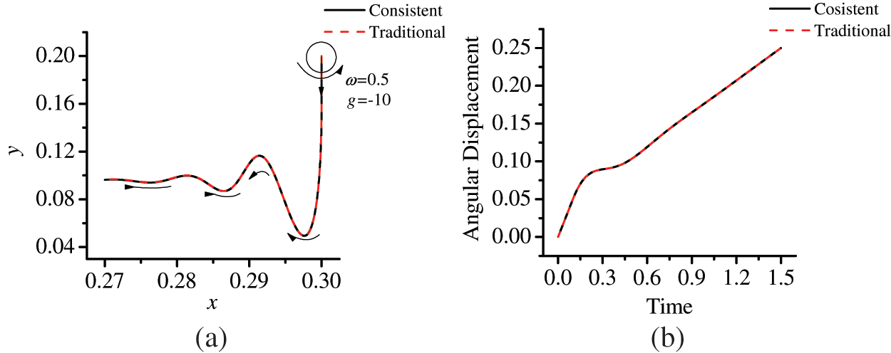
Figure 4: The time history of ball’s motion with different tangential displacement evaluation methods: (a) Translational motion of ball’s center (b) Angular displacement
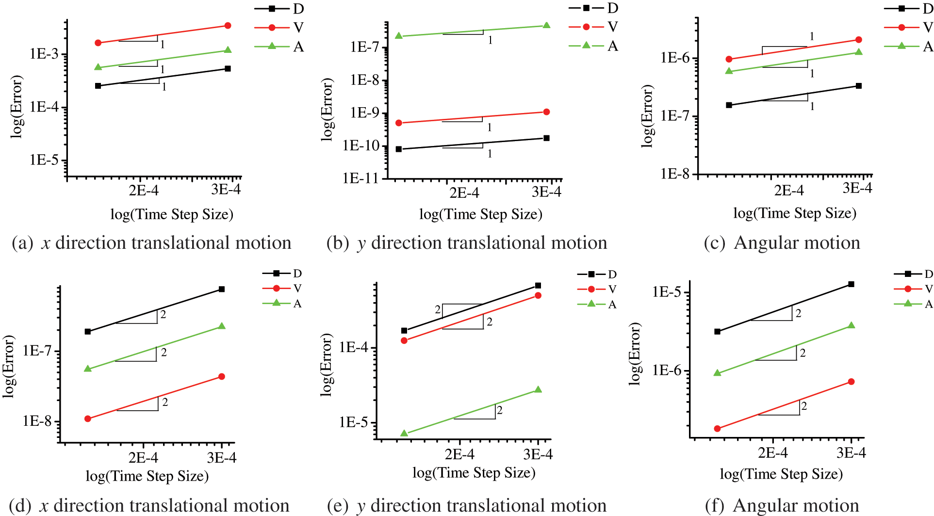
Figure 5: Time accuracy plots of the central difference method with traditional tangential displacement evaluation method (top) and consistent tangential displacement evaluation method (bottom)
Problem Description: The numerical example chosen in this section is that of a simple granular cube drop of particles in three-dimensional space, as shown in Fig. 6. The granular cube has dimensions of 0.3 length
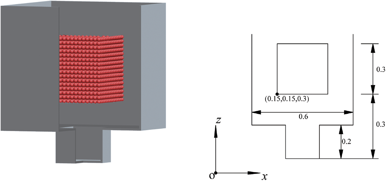
Figure 6: Schematic of the problem (Numerical example)
In this section, the consistent time level implementation and preserving the second-order time accuracy for the presented results in this section are as follows for a wide variety of time integrators in the present unified framework. They yield no overshoot in displacement or no overshoot in velocity or no overshoot in both displacement and velocity for a given set of initial conditions:
• CDM-T: Central Difference Method with traditional tangential displacement evaluation. Note that the central difference method has been proved to be equivalent to the GS4-II U0-based family with
• CDM-C: Central Difference Method with consistent tangential displacement evaluation.
• V0(1, 1, 0)-C: GS4-II V0-based family with
• U0/V0(0, 1, 0)-C: GS4-II U0-based family or V0-based family with
Numerical Setting and Computational Cost
In order to capture particle contacts, the time step size used in DEM type simulations is always required to be very small. This implies that the implicit time integration schemes are not necessary in the general DEM simulations. Therefore, in this work, all the schemes listed are explicit and the time step size is
Numerical Results and Discussion
Three-dimensional snapshots with the granular velocity filed values at six different times (

Figure 7: Velocity fields at different time by CDM-C
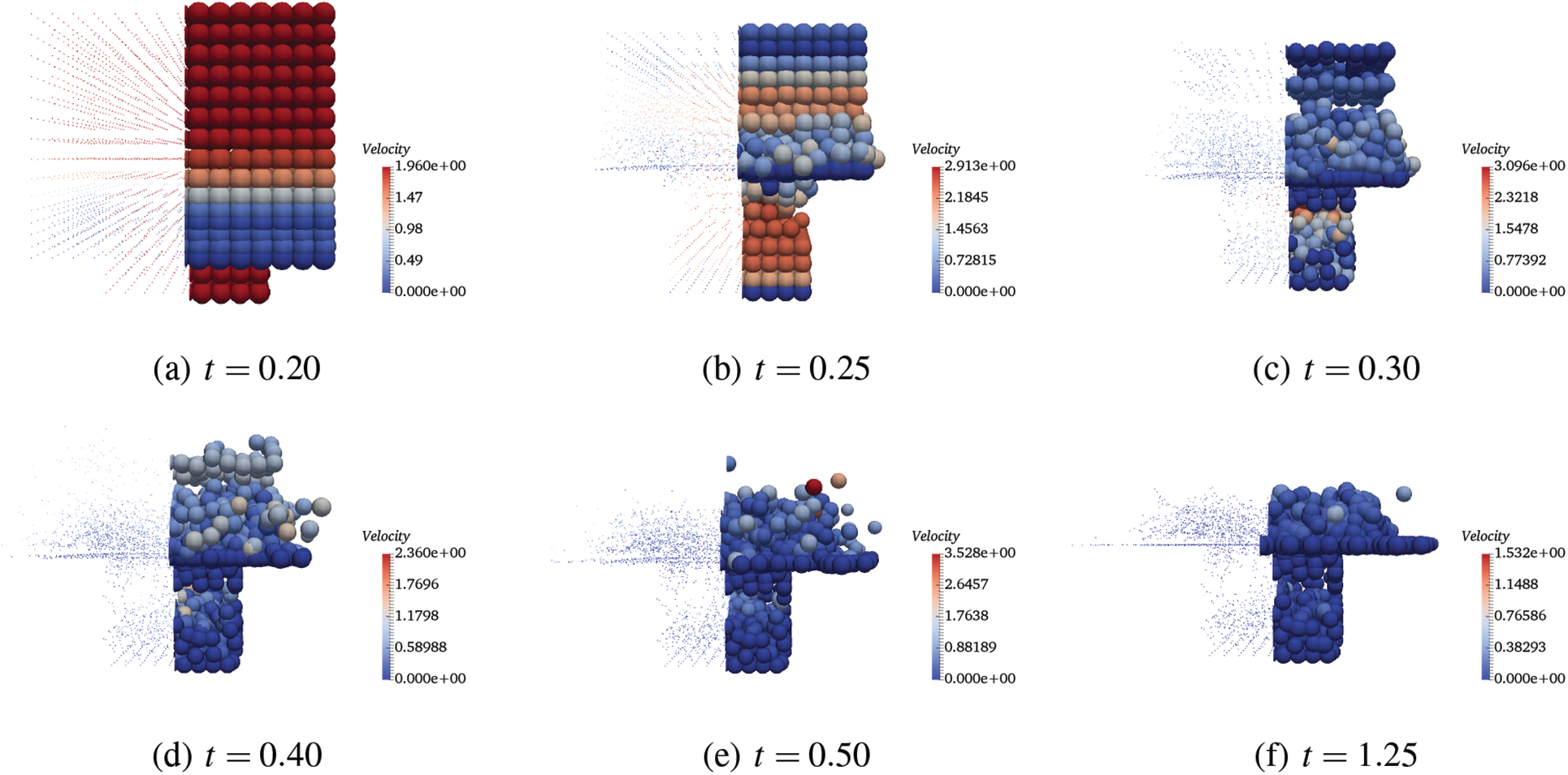
Figure 8: Velocity fields at different time by CDM-T
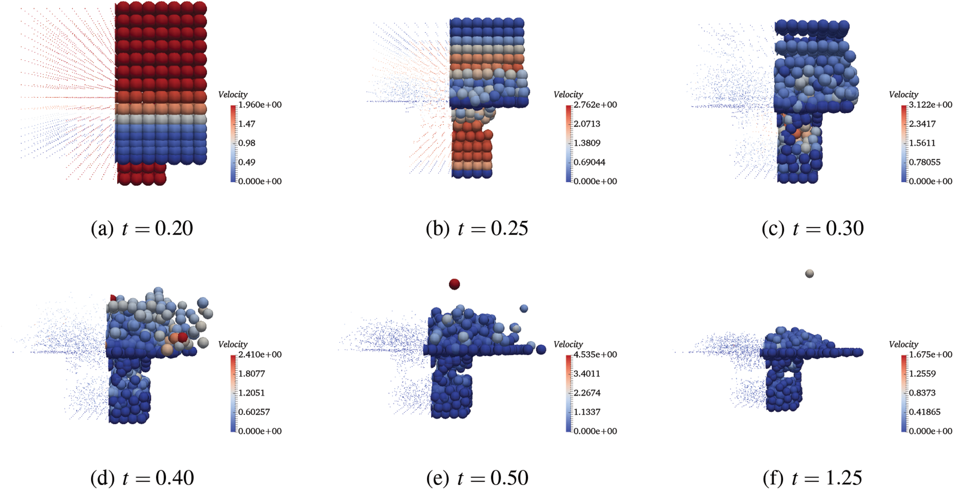
Figure 9: Velocity fields at different time by V0(1, 1, 0)-C
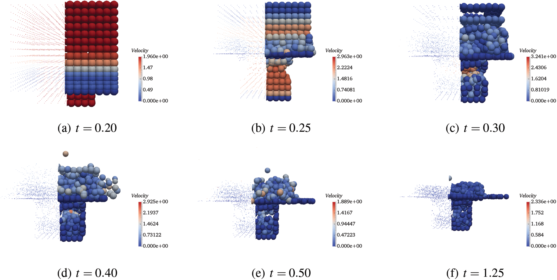
Figure 10: Velocity fields at different time by U0/V0(0, 1, 0)-C
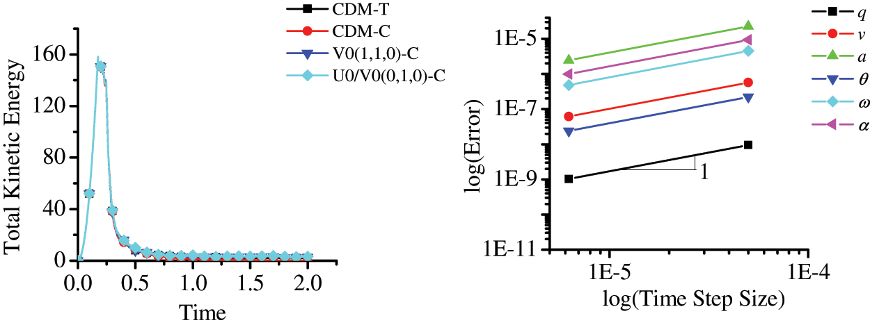
Figure 11: Left: total kinetic energy. Right: time accuracy plots of central different method with traditional tangential displacement evaluation
The time accuracy for translational and rotational position, velocity and acceleration of the central difference method with the traditional tangential displacement evaluation shows only first-order time accuracy in Fig. 11 (right). However, alternately, Fig. 12 shows the second-order time accuracy for translational position, velocity and acceleration of different time integration schemes selected within the GS4-II family with the proposed consistent tangential displacement evaluation. All the schemes show the second-order time accuracy in both translational and rotational motion. It is to be noted however, that using central difference method in solving the second-order ODE, it is supposed to yield second-order accuracy in time. According to the time convergence order from different tangential displacement evaluations, it implies that the drawback via the traditional tangential displacement evaluation in DEM type method is not at the same time level as the algorithm and has significant influence on the whole system’s time accuracy. In other words, only when the tangential displacement evaluation is evaluated at a consistent time level corresponding to the selected time integration scheme within the unified framework described, the results are completely reliable and the time integration schemes are implemented correctly and efficiently maintaining second-order time accuracy with improvement in physics.
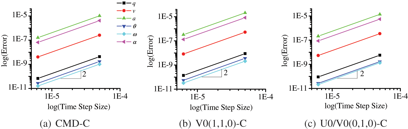
Figure 12: Time accuracy plots of different selected schemes within GS4-II family: q, v and a are translational position, velocity and acceleration, respectively.
In this work, a consistent tangential displacement evaluation approach is proposed under the framework of the unified second-order time integrators GS4-II family for improving discrete element method (DEM) simulations. The newly proposed approach is derived and designed to maintain the simplicity and generalization of the GS4-II family. Comparing it with the traditional tangential displacement evaluation method, the proposed consistent time level implementation approach can be easily implemented and yields the correct algorithmic tangential displacement at the same time level as in the time integrations via using the same parameters (
Acknowledgement: We appreciate all the constructive comments and suggestions from editors and reviewers.
Funding Statement: The authors received no specific funding for this study.
Conflicts of Interest: The authors declare that they have no conflicts of interest to report regarding the present study.
References
1. Cundall, P. A., Strack, O. D. L. (1979). A discrete numerical model for granular assemblies. Geotechnique, 29, 47–65. DOI 10.1680/geot.1979.29.1.47. [Google Scholar] [CrossRef]
2. Luding, S. (1997). Stress distribution in static two-dimensional granular model media in the absence of friction. Physical Review E, 55, 4720–4729. DOI 10.1103/PhysRevE.55.4720. [Google Scholar] [CrossRef]
3. Baxter, J., Tüzün, U., Burnell, J., Heyes, D. M. (1997). Granular dynamics simulations of two-dimensional heap formation. Physical Review E, 55(3), 3546. DOI 10.1103/PhysRevE.55.3546. [Google Scholar] [CrossRef]
4. Zhou, Y. C., Xu, B. H., Zou, R., Yu, A. B., Zulli, P. (2003). Stress distribution in a sandpile formed on a deflected base. Advanced Powder Technology, 14(4), 401–410. DOI 10.1163/156855203769710636. [Google Scholar] [CrossRef]
5. Fazekas, S., Kertész, J., Wolf, D. E. (2005). Piling and avalanches of magnetized particles. Physical Review E, 71(6), 061303. DOI 10.1103/PhysRevE.71.061303. [Google Scholar] [CrossRef]
6. Li, Y., Xu, Y., Thornton, C. (2005). A comparison of discrete element simulations and experiments for ‘sandpiles’ composed of spherical particles. Powder Technology, 160(3), 219–228. DOI 10.1016/j.powtec.2005.09.002. [Google Scholar] [CrossRef]
7. Yen, K. Z. Y., Chaki, T. (1992). A dynamic simulation of particle rearrangement in powder packings with realistic interactions. Journal of Applied Physics, 71(7), 3164–3173. DOI 10.1063/1.350958. [Google Scholar] [CrossRef]
8. Zhang, Z. P., Liu, L. F., Yuan, Y. D., Yu, A. B. (2001). A simulation study of the effects of dynamic variables on the packing of spheres. Powder Technology, 116(1), 23–32. DOI 10.1016/S0032-5910(00)00356-9. [Google Scholar] [CrossRef]
9. Latham, J. P., Lu, Y., Munjiza, A. (2001). A random method for simulating loose packs of angular particles using tetrahedra. Geotechnique, 51(10), 871–879. DOI 10.1680/geot.2001.51.10.871. [Google Scholar] [CrossRef]
10. Silbert, L. E., Grest, G. S., Landry, J. W. (2002). Statistics of the contact network in frictional and frictionless granular packings. Physical Review E, 66(6), 061303. DOI 10.1103/PhysRevE.66.061303. [Google Scholar] [CrossRef]
11. Munjiza, A. A. (2004). The combined finite-discrete element method. West Sussex, UK: John Wiley & Sons. [Google Scholar]
12. An, X. Z., Yang, R. Y., Dong, K. J., Zou, R. P., Yu, A. B. (2005). Micromechanical simulation and analysis of one-dimensional vibratory sphere acking. Physical Review Letters, 95(20), 205502. DOI 10.1103/PhysRevLett.95.205502. [Google Scholar] [CrossRef]
13. Just, S., Toschkoff, G., Funke, A., Djuric, D., Scharrer, G. et al. (2013). Experimental analysis of tablet properties for discrete element modeling of an active coating process. AAPS PharmSciTech, 14(1), 402–411. DOI 10.1208/s12249-013-9925-5. [Google Scholar] [CrossRef]
14. Lewis, R. W., Gethin, D. T., Yang, X. S., Rowe, R. C. (2005). A combined finite-discrete element method for simulating pharmaceutical powder tableting. Numerical Methods in Engineering, 62, 853–869. DOI 10.1002/(ISSN)1097-0207. [Google Scholar] [CrossRef]
15. Buchholtz, V., Pöschel, T., Tillemans, H. J. (1995). Simulation of rotating drum experiments using non-circular particles. Physica A: Statistical Mechanics and its Applications, 216(3), 199–212. DOI 10.1016/0378-4371(95)00045-9. [Google Scholar] [CrossRef]
16. Pöschel, T., Buchholtz, V. (1995). Complex flow of granular material in a rotating cylinder. Chaos, Solitons and Fractals, 5(10), 1901–1912. DOI 10.1016/0960-0779(94)00193-T. [Google Scholar] [CrossRef]
17. Sakai, M., Shibata, K., Koshizuka, S. (2006). Development of a criticality evaluation method involving the granular flow of the nuclear fuel in a rotating drum. Nuclear Science and Engineering, 154(1), 63–73. DOI 10.13182/NSE06-A2618. [Google Scholar] [CrossRef]
18. Portillo, P. M., Muzzio, F. J., Ierapetritou, M. G. (2007). Hybrid DEM-compartment modeling approach for granular mixing. AIChE Journal, 53(1), 119–128. DOI 10.1002/(ISSN)1547-5905. [Google Scholar] [CrossRef]
19. Mishra, B. K., Rajamani, R. K. (1992). The discrete element method for the simulation of ball mills. Applied Mathematical Modelling, 16, 598–604. DOI 10.1016/0307-904X(92)90035-2. [Google Scholar] [CrossRef]
20. Inoue, T., Okaya, K. (2012). Grinding mechanism of centrifugal mills-A simulation study based on the discrete element method. Comminution, 1994, 425. DOI 10.1016/0301-7516(95)00049-6. [Google Scholar] [CrossRef]
21. Gudin, D., Kano, J., Saito, F. (2007). Effect of the friction coefficient in the discrete element method simulation on media motion in a wet bead mill. Advanced Powder Technology, 18(5), 555–565. DOI 10.1163/156855207782146625. [Google Scholar] [CrossRef]
22. Sun, X., Sakai, M., Yamada, Y. (2013). Three-dimensional simulation of a solid-liquid flow by the DEM-SPH method. Journal of Computational Physics, 248, 147–176. DOI 10.1016/j.jcp.2013.04.019. [Google Scholar] [CrossRef]
23. Schwartz, S. R., Michel, P., Richardson, D. C. (2013). Numerically simulating impact disruptions of cohesive glass bead agglomerates using the soft-sphere discrete element method. Icarus, 226(1), 67–76. DOI 10.1016/j.icarus.2013.05.007. [Google Scholar] [CrossRef]
24. Guo, Y., Wassgren, C., Hancock, B., Ketterhagen, W., Curtis, J. (2015). Computational study of granular shear flows of dry flexible fibres using the discrete element method. Journal of Fluid Mechanics, 775, 24–52. DOI 10.1017/jfm.2015.289. [Google Scholar] [CrossRef]
25. Guo, Y., Curtis, J. S. (2015). Discrete element method simulations for complex granular flows. Annual Review of Fluid Mechanics, 47, 21–46. DOI 10.1146/annurev-fluid-010814-014644. [Google Scholar] [CrossRef]
26. Munjiza, A., Owen, D., Bicanic, N. (1995). A combined finite-discrete element method in transient dynamics of fracturing solids. Engineering Computations, 12(2), 145–174. DOI 10.1108/02644409510799532. [Google Scholar] [CrossRef]
27. Peters, B. (2013). The extended discrete element method (XDEM) for multi-physics applications. Scholarly Journal of Engineering Research, 2, 1–20. [Google Scholar]
28. Wang, Y., Tamma, K., Maxam, D., Xue, T., Qin, G. (2021). An overview of high-order implicit algorithms for first-/second-order systems and novel explicit algorithm designs for first-order system representations. Archives of Computational Methods in Engineering, 28(5), 3593–3619. DOI 10.1007/s11831-021-09536-3. [Google Scholar] [CrossRef]
29. Xue, T., Wang, Y., Aanjaneya, M., Tamma, K. K., Qin, G. (2021). On a generalized energy conservation/dissipation time finite element method for Hamiltonian mechanics. Computer Methods in Applied Mechanics and Engineering, 373, 113509. DOI 10.1016/j.cma.2020.113509. [Google Scholar] [CrossRef]
30. Shimada, M., Tamma, K. K. (2013). Explicit time integrators and designs for first/second order linear transient systems. Encyclopedia of Thermal Stresses, 3, 1524–1530. DOI 10.1007/978-94-007-2739-7_764. [Google Scholar] [CrossRef]
31. Atluri, S. N., Han, Z. D., Shen, S. (2003). Meshless local petrov-galerkin (MLPG) approaches for solving the weakly-singular traction and displacement boundary integral equations. Computer Modeling in Engineering & Sciences, 4(5), 507–518. DOI 10.3970/cmes.2003.004.507. [Google Scholar] [CrossRef]
32. Han, Z. D., Atluri, S. (2004). Meshless local petrov-galerkin (MLPG) approaches for solving 3D problems in elasto-statics. Computer Modeling in Engineering & Sciences, 6, 169–188. DOI 10.3970/cmes.2004.006.169. [Google Scholar] [CrossRef]
33. Long, S., Atluri, S. N. (2002). A meshless local petrov-galerkin method for solving the bending problem of a thin plate. Computer Modeling in Engineering & Sciences, 3(1), 53–64. DOI 10.3970/cmes.2002.003.053. [Google Scholar] [CrossRef]
34. Xue, T., Zhang, X., Tamma, K. K. (2018). A two-field state-based peridynamic theory for thermal contact problems. Journal of Computational Physics, 374, 1180–1195. DOI 10.1016/j.jcp.2018.08.014. [Google Scholar] [CrossRef]
35. Xue, T., Zhang, X., Tamma, K. K. (2019). A non-local dissipative lagrangian modelling for generalized thermoelasticity in solids. Applied Mathematical Modelling, 73, 247–265. DOI 10.1016/j.apm.2019.04.004. [Google Scholar] [CrossRef]
36. Matuttis, H., Chen, J. (2014). Understanding the discrete element method: Simulation of non-spherical particles for granular and multi-body systems, 1st edition. Chichester, UK: John Wiley. [Google Scholar]
37. Tsuji, Y., Tanaka, T., Ishida, T. (1992). Lagrangian numerical simulation of plug flow of cohesionless particles in a horizontal pipe. Powder Technology, 71, 239–250. DOI 10.1016/0032-5910(92)88030-L. [Google Scholar] [CrossRef]
38. Mindlin, R. D. (1949). Compliance of elastic bodies in contact. Journal of Applied Mechanics, 16, 259–268. DOI 10.1115/1.4009973. [Google Scholar] [CrossRef]
39. Mindlin, R. D., Deresiewicz, H. (1953). Elastic spheres in contact under varying oblique forces. Journal of Applied Mechanics, 20, 327–344. DOI 10.1115/1.4010702. [Google Scholar] [CrossRef]
40. Har, J., Tamma, K. K. (2012). Advances in computational dynamics of particles, materials and structures. Chichester, UK: John Wiley. [Google Scholar]
41. Tamma, K. K., Har, J., Zhou, X., Shimada, M., Hoitink, A. (2011). An overview and recent advances in vector and scalar formalisms: Space/time discretizations in computational dynamics: A unified approach. Archives of Computational Methods in Engineering, 18, 119–283. DOI 10.1007/s11831-011-9060-y. [Google Scholar] [CrossRef]
42. Shimada, M., Hoitink, A., Tamma, K. K. (2015). The fundamentals underlying evaluation of acceleration computations for general dynamic applications: Issues and noteworthy perspectives. Computer Methods in Applied Mechanics and Engineering, 104(2), 133–158. DOI 10.3970/cmes.2015.104.133. [Google Scholar] [CrossRef]
43. Hughes, T. J. R. (2000). The finite element method: Linear static and dynamic finite element analysis. Mineola, New York: Dover Publications. [Google Scholar]
Cite This Article
 Copyright © 2023 The Author(s). Published by Tech Science Press.
This work is licensed under a Creative Commons Attribution 4.0 International License , which permits unrestricted use, distribution, and reproduction in any medium, provided the original work is properly cited.
 Downloads
 Citation Tools