A Detection Method of Bolts on Axlebox Cover Based on Cascade Deep Convolutional Neural Network

1  Introduction

As the rapidly developing of metro in China, a total of 8,553.40 km of urban rail transit lines, including 6,737.23 km of metro, have been put into operation in 49 cities in mainland China [1]. However, while metro brings convenience to life, the ensuing safety operation problems cannot be ignored. Any minor malfunction may cause great safety hazards during the high-speed operation of the metro. Although major safety accidents during metro operation rarely occur in China, emergency train pickups and delays due to malfunctions do occur from time to time [2].

Bolts have the advantages of compact structure, easy disassembly, high connection force and repeated use, which have great advantages in the use of equipment and ensure the reliability and stability of the bogie system of metro vehicles [3–5]. The bolted joint on the axlebox cover mainly consists of a pair of bolts and nuts and several connecting parts. In theory, the bolt joint is kept stable by rotating the nut and bolt relative to each other, elongating the bolt and compressing the joint part to form a frictional self-locking. In this case, the bolt tension is the pressure on the contact surface of the joint and the bolt [6]. In fact, the bolt tension decreases due to repeated relative sliding wear of the joint or plastic deformation of the bolt and the joint, which can directly lead to the loss of function of the joint [7–9]. The loosening caused by the decrease of bolt tension is called bolt loosening [10]. Loose bolts can cause a series of problems such as separation, falling off and sliding of the joint, resulting in displacement and collision of the joint [11]. At present, there are two main cases of bolt loosening: rotational loosening and non-rotational loosening. The loosening caused by the relative rotation between the bolt and the joint is called rotational loosening, while the loosening caused by the plastic deformation of the bolt itself or the joint becomes non-rotational loosening. Currently, most of the loose bolts on the axlebox cover are rotating loose. Therefore, non-rotational loosening is not considered in this paper.

The traditional daily inspection mode of metro vehicles is manual inspection, but this mode is inefficient and has a high rate of leakage and false detection. With the development of nondestructive testing (NDT), the daily inspection mode of subway vehicles has changed from manual inspection to machine inspection, such as machine inspection based on nondestructive testing [12]. At present, bolt detection based on NDT methods is mainly divided into two categories: ultrasonic-based NDT [13] and computer vision-based NDT [14–16].

Due to the development of signal processing, more several methods had been applied on the bolt detection. Xu et al. [17] built the variational modal decomposition (VMD) combined morphological filtering principle into the bolt detection signal analysis method based on morphological filtering and VMD methods, which was implemented for bolt fault detection. Ramasso et al. [18] explicitly represented the cluster onset in Gaussian mixture models (GMM) and, by modifying the internal criteria of these models, which was used to describe the loosening phenomenon of bolted structures under vibration. Guo et al. [19] introduced an improved complete ensemble empirical mode decomposition (ICEEMD) to the bolt detection signal analysis, which can effectively identify the reflected signal at the end of the bolt by eliminating the noise of the intrinsic mode function (IMF) through a wavelet soft threshold denoising technique. These ultrasonic-based NDT methods focus on detecting faults, looseness and other abnormal conditions inside the bolt, and they are usually better in terms of detection accuracy but less efficient.

Apart from these signal processing methods, computer vision-based on NDT and deep learning is also widely used in bolt detection. Sun et al. [20] proposed a binocular vision-based method for loose bolt detection in trains, combining convolutional neural networks (CNN) to bring up the sub-pixel edges of bolt caps and surfaces and determine whether the bolt is faulty based on the calculated distance compared with the reference value. Song et al. [21] proposed a method combining traditional image algorithms and deep learning for the detection of freight train carpenter bolts, and used stacked autoencoders (SAEs) to provide pre-trained weights for convolutional neural networks to achieve effective feature extraction in the convolutional layer, which helps to speed up the training. Yang et al. [22] improved the overall performance of the network by adding an attention mechanism to the feature extraction layer of the CNN. Marino et al. [3] determined whether the bolts were missing by acquiring bolt images from a digital line-scan camera while preprocessing them according to two discrete wavelet transforms, which were then provided to two multilayer perceptron neural classifiers (MLPNCs). Cha et al. [23] used Region Proposal Network (RPN) tandem ZF-net with Faster Region-Convolutional Neural Network (Faster R-CNN) for high accuracy detection of various cracks and missing bolts. Huynh et al. [24] similarly used deep learning network of Region-Convolutional Neural Network (R-CNN) to detect bolts. Most of these detection methods use object detection to locate to each bolt region, with strong fitting and generalization capabilities, as well as robustness. It can be concluded that the computer vision-based NDT focuses more on considering whether the bolt is missing from the positioning result and did not take into account whether the bolt is loose or not based on the characteristics of the positioned bolt.

For bolt detection, computer vision-based NDT can quickly detect whether the bolt is missing, while ultrasonic-based NDT is more inclined to detect whether the bolt is loose. Since the efficiency of ultrasonic inspection is relatively low and cannot meet the rapid daily inspection of vehicles, the object positioning technology of computer vision is mainly used to detect the bolt status. Admittedly, measuring bolt loosening using computer vision is a popular research topic and some attempts have been made by researchers. Wang et al. [25] used CNN digital recognition to identify bolt positioning and applied Hough transform line detection to detect bolt rotation angle for final rotational loosening detection by comparing with the initial position of the fastened bolt. Zhao et al. [26] used Single Shot Multiple Box Detection (SSD) to position the bolt and the numbers on it, and the angle is calculated by the rotation of the numbers relative to its initial position for rotational loosening detection of the bolt. They did pioneer some ideas based on computer vision to detect loose bolts, but their methods start the process directly from the bolt, without the process of how to locate the bolt from the overall data set in the first place, and they still have a large error. Therefore, this work aims to be able to make a complete computer vision-based system that can start from collecting data, can pinpoint all the bolts from the background, and can perform loose detection of the bolts. Recently, the detection method of connecting multiple deep learning networks in series, using each network on different functions of detection, and combining them into a cascade network has been proposed, opening up new ideas for deep learning-based detection methods. Zhang et al. [27] combined P-Net for coarse localization, R-Net for fine localization, and O-Net for point localization in series to form a cascade network for face recognition detection. Moreover, Chen et al. [28] applied a series of methods for defects detections. Firstly, they used SSD for joint localization, then YOLO for fastener localization, and finally DCNN was used to classify the defects. Similarly, Wang et al. [29] used YOLOv3, which is based on a modified Deblur block, for primary localization of the joint and secondary localization of each component of the joint, and finally semantic segmentation of the components using deeplabv3.

In general, cascade networks are highly variable and combinatorial, suitable for multifaceted detection of objects, but do not allow for end-to-end structures. Studying bolt loosening detection from the perspective of computer vision, a cascade network based on deep learning for axle box cover marker line bolt detection and angle measurement of urban rail transit metro vehicles is proposed in combination with the theory related to deep learning. An improved SSD [30] network based on Residual Network-50 (ResNet-50) [31] with Convolutional Block Attention Module (CBAM) [32] was proposed and used to locate and segment four types of bolts from the original image of the axlebox cover. After selecting the bolts with marker lines from all the localization results, based on the saliency detection network and Pyramid Feature Attention Network (PFA) [33], the Squeeze Excitation (SE) [34] module is applied to extract the high-level features, while the Double Attention (DA) module [35] and the A2-PFN model is proposed to extract the low-level and marker line features of the bolts to generate the saliency map. At present, the metro operating company stipulates the marker line on the axlebox cover which can be located in the horizontal position for the tightening state. This indicates that the bolt tension can reach its maximum value when the marker line is in the horizontal position. The special case that the bolt rotates for one week and then reaches the horizontal position again can be disregarded because the metro vehicles are serviced very frequently and it is easy to detect a bolt that has the possibility of rotating loose. Therefore, based on the marker line prominence diagram, the rectangular approximation method is used to measure the angle of the marker line deviation from the horizontal line, and a new method to discern whether the bolt is loose or not, the angle table method, is proposed.

This paper makes the following contributions:

1.    Optimizing the SSD network with ResNet-50 and CBAM to improve the detection accuracy for small bolts, while ensuring better detection speed to guarantee that all bolts with marker lines can be acquired as much as possible.

2.    After selecting the bolts with marker lines from all localization results, the SE module and DA module are applied to extract the marker line features of high and low levels respectively, and A2-PFN is proposed to extract the marker line features of the bolts and generate the saliency map.

3.    The rectangular approximation method is proposed to frame the extracted feature position, and the average of the angle between the two long sides of the rectangular frame deviating from the horizontal position is used as the angle of deviation of the marker line and the angle table is drawn accordingly.

In the following sections of this paper, method overview is introduced in Section 2, including the general stages as well as the specific theory of each stage. Section 3 shows some experimental results of our method and comparison has been done with other methods. Finally, Section 4 gives the conclusion and outlook.

2  Method Overview

The proposed method can be divided into three stages. The main objective of the first stage of the method in this paper is to segment all types of bolts from the original data set faster, more accurately and more completely. As a result, the object localization is used. The saliency detection is used during the second stage to locate the marker lines of the bolts. Moreover, the main purpose of the third stage is to distinguish the tightness of the bolts based on measuring their angles using the rectangular approximation method according to the marker line regions. The specific method flow described below is shown in Fig. 1.

Figure 1: Process of proposed method

1.    In the first stage, an improved SSD network based on ResNet-50 with CBAM is used to segment out all kinds of bolt regions, such as Bolt_A, Bolt_B, Bolt_C and Bolt_D in Fig. 2. From them, the bolts with marker lines, referring to Bolt_A and Bolt_B, are filtered out and used for processing in the second stage.

2.    In the second stage, A2-PFN is proposed to detect the saliency of the marker line regions and generate the corresponding saliency maps.

3.    Based on the feature that the bolt is tightened when the marker lines are in the horizontal position, the angle of deviation of the marker line from the horizontal line is measured by the rectangular approximation method based on the saliency regions obtained in the second stage and the angle table is drawn.

4.    According to the angle table, it is stipulated that the upper and lower deviation from the horizontal position within a certain angle is the tightening state, and within a certain angle is the loosening state, so as to determine whether the bolts with marker lines of any axle box cover have the risk of loosening.

Figure 2: Four types of bolts

2.1 Object Localization Stage

2.1.1 Related Works

Currently, object detection is mainly used to implement object positioning technology. Object detection refers to finding regions of interest from videos or images and marking them, and extracting features by algorithms to identify and locate specific classes of objects. In recent years, deep CNNs have achieved breakthrough research results in the field of object detection, and their detection accuracy and speed have been improved, such as R-CNN [36], Fast Region-Convolutional Neural Network (Fast R-CNN) [37], Faster R-CNN [38], You Only Look Once (YOLO) [39], Single Shot Multibox Detector (SSD) [30], etc. At present, deep learning-based object detection algorithms can be broadly divided into two categories: two-stage and one-stage. R-CNN, Fast-RCNN, and Faster-RCNN are a series of classical two-stage algorithms, while YOLO and SSD are representatives of one-stage algorithms.

The two-stage algorithm is a regression-based algorithm that consists of two stages: the generation of anchor frames through the network and the regression of the anchor frames through processing for positioning. Dong et al. [40] developed the soft non-maximal suppression (Soft-NMS) algorithm to improve the segmentation accuracy of Mask Region-Convolutional Neural Network (Mask R-CNN). Chen et al. [41] proposed a new graph attention module (GAM) based on R-CNN, which enables inference across heterogeneous nodes by operating directly on graph edges. Zhang et al. [42] proposed a post-processing layer structure for removing the irrelevant parts of the two-stage segmentation results. Wang et al. [43] combined R-CNN with adaptive RF techniques to form a depth model from multiple gated recursive convolutional layers and achieved better results than R-CNN. Narasimhaswamy et al. [44] fused Mask R-CNN with two different attentional mechanisms, enabling it to densely aggregate features that will separate regions and adaptively select salient features from this region. Deshapriya et al. [45] proposed a new convolutional neural network architecture (Vec2Instance), a framework that enables convolutional neural networks to efficiently estimate the complex shapes around the centroids of instances with improved accuracy. Cao et al. [46] addressed the balance between feature maps and perceptual fields at high resolution by introducing an attention mechanism. Generally, detection accuracy of two-stage algorithm is good, but this kind of algorithm cannot reach the real-time object detection requirements, the computation of the generated area is still huge, and there are still big obstacles to the detection of small objects.

The one-stage algorithm is a direct localization regression algorithm, which reduces the number of staging steps than the two-stage algorithm, so the detection speed is faster. Liu et al. [47] proposed a distinguishable image processing (DIP) module with an end-to-end approach to jointly learn CNN-PP and YOLOv3 for the task of balancing image enhancement and object detection. Ganesh et al. [48] achieved multi-scale feature interaction by exploiting the missing combinatorial connections between various feature scales in the existing state-of-the-art methods, and enhanced both accuracy and detection speed on the improved YOLOv4. Khokhlov et al. [49] improved the detection accuracy with less computational overhead by slightly modifying the YOLOv3-tiny with the help of a priori knowledge about the scene geometry. Yi et al. [50] improved SSD by establishing feature relationships in the spatial space of the feature map and learning to highlight useful regions on the feature map with global relationship information while suppressing irrelevant information. Shi et al. [51] proposed a new Fluff module to mitigate the drawbacks of multi-scale let fusion methods and facilitate multi-scale object detection, combining SSD with the Fluff module to obtain significant efficiency and accuracy. Moreover, Tian et al. [52] proposed a novel one-stage object detection algorithm without anchor box, which avoids all hyperparameters associated with the anchor box and achieves improved detection accuracy. Currently, one-stage algorithm still has great difficulties in the detection of small objects, and the bolt happens to have the characteristics of small size and few features, so the choice of one-stage algorithm is also a challenge for bolt detection.

In practical application, high precision, high localization accuracy and high detection efficiency are essential. Although the two-stage algorithm has a high accuracy of localization, its prediction efficiency is very worrying and far from meeting the requirements. The one-stage algorithm, on the other hand, has certain problems in localization accuracy, but the detection efficiency can meet the requirements of this work. Considering the advantages and disadvantages of these algorithms, the one-stage algorithm with higher detection efficiency, the SSD, is chosen as the base algorithm and is improved for its localization accuracy and precision because of its weakness to small object detection.

2.1.2 Limitations of SSD Network and Ideas for Improvement

SSD is a classical one-stage object localization algorithm, which is better for large object localization, with a smaller model and faster detection speed. This is because SSD performs object localization and classification on each convolutional layer, and Fast Non-Maximum Suppression (Fast NMS) performs filtering and outputs the final result. The object localization on multi-scale feature map is equivalent to many more bounding boxes with wide to high ratio, and the wide to high ratio of large bolt region is varied, which happens to greatly improve the generalization ability. However, when the original SSD network is used to train the axle box cover dataset, it is prone to the situation that the error firstly decreases and then increases during training, resulting in the BOLT_C with a smaller object region not being recognized, as shown in Fig. 3.

Figure 3: Result of bolt detection using the original SSD

This is not a problem triggered by overfitting, but the network becomes deeper making it difficult to train small objects [53]. Since CNN has the property that the deeper the network depth is, the less detailed features are needed to detect small bolts like BOLT_C. There is little such detailed information left in the deep network, and the final detection result is naturally poor. In contrast, shallow networks in CNN with large feature mapping size, small perceptual field, and rich information of detailed features are more discriminative for the object localization regression subtask [54], which is suitable for small objects with simple features. And the framework of the basic SSD network is a Visual Geometry Group Network-16 (VGG-16) network for image feature extraction, to which four additional layers of auxiliary structures are added to generate feature maps of different dimensions, and finally predictions are made on a total of six feature maps. Therefore, based on the previously mentioned shallow network features, this paper improves the shallow network for the SSD network, i.e., the convolutional layer that generates feature maps 1&2.

In addition, VGG16, as the backbone part of the SSD network, has the defects of long training time, many training parameters, and easy degradation problems during the training process. Inspired by Fu et al. [55], who used ResNet-101 as well as FPN to be the backbone for object localization, this paper uses ResNet-50 to replace VGG-16 as the backbone part of the whole network. The design idea of residual network is to use shortcut connection to make the residual possible and use constant mapping to make the network deeper and reduce the computational parameters [31], which is equivalent to making the network more accurate and simplifying the network, so the use of residual network can compensate this defect of the original SSD to some extent.

2.1.3 Specific Improvement Strategies

The residual block is basically designed with reference to the original ResNet50, and instead of choosing the design of two 3 × 3 convolutional layers, the design of 1 × 1 + 3 × 3 + 1 × 1 convolutional layer is chosen, whose accuracy results will not change, with the aim of reducing the computational effort.

In the framework of the basic SSD network, the channels of the feature maps are specified as 1024, 512, 512, 256, 256 and 256, respectively. In order to match the channels of the six feature maps set by SSD, this paper discards Conv5_x and its subsequent average pooling layers, fully-connected layers, and softmax layers in the basic ResNet50 model, i.e., the layer structure of Conv1_x to Conv4_x is used. In particular, this paper adjusts the stride from 2 to 1 in Conv4_x. This operation changes the output of feature map 1 from 19 × 19 × 1024 to 38 × 38 × 1024, which corresponds to the size of feature map 1 of 38×38 in the framework of the basic SSD network.

In order to perform faster and more accurate localization of the bolt regions, inspired by the work of Woo et al. [32] and Han et al. [54], this paper adds an additional CBAM module after Conv4_x. The CBAM module can be divided into two sub-modules before and after, the former for channel attention (CA) and the latter for spatial attention (SA). Since each channel of the feature map is considered as a feature detector, the CA focuses on the semantic features of a given input image [32]. In addition, with a large amount of detail contained in the shallow feature map, employing SA allows more attention to be paid to the details of object regions rather than considering all spatial details equally. In particular, inspired by the channels weighted block (CWB) employed by Song et al. [56], instead of the traditional operation of generating an effective feature descriptor to highlight detail regions through average pooling and maximum pooling, this paper applies two convolutional layers, one with a kernel of 1×k, and the other with a kernel of k×1, to obtain spatial attention. This is in consideration of the fact that the bolts in the axle box cover dataset vary in size and degree of detail, and that the pooling operation using only the traditional method is likely to ignore this detail, and thus a convolution operation is used instead. The improved CBAM module is shown in Fig. 4, and the equations of CA and SA are:

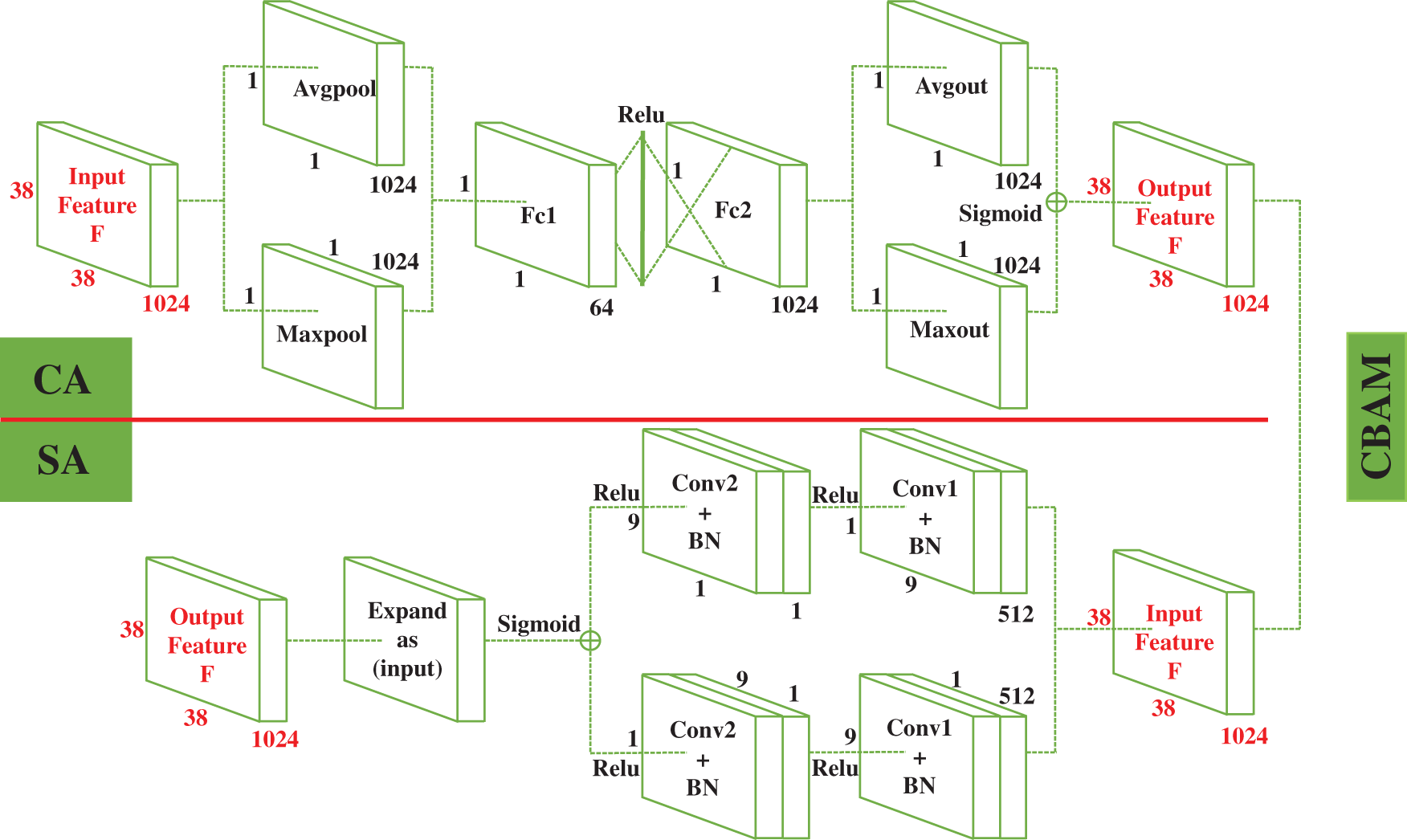
Figure 4: CBAM module with improved SA

CA=σ(MLP(AvgPool(F))+MLP(MaxPool(F)))=σ(W1(W0(Favgc))+W1(W0(Fmaxc)))(1)

SA=σ(conv2(conv1(F,W0),W1)+conv1(conv2(F,W1),W0))(2)

where σ denotes the sigmoid function, MLP denotes the multilayer perceptron, conv1 and conv2 denote the convolutional layers with structures 1×k×C and k×1×1, respectively, for a particular feature map F∈RW×H×C with W0∈RC/r×C, W1∈RC×C/r, where C is the number of channels, r is the degradation ratio, Favgc and Fmaxc denote the average pooling feature and the maximum pooling feature, respectively.

Finally, the extra layer structure is improved. Inspired by Li et al. [57], this paper adds a batch normalization (BN) layer, which is not used in the basic SSD network, after each convolutional layer in the last four extra layer structures to normalize the feature information and reduce the variability. The main role of BN layer is to alleviate the gradient disappearance problem in training, as well as to speed up the training of the model.

Combining the problems that occur when the original SSD network is used to detect bolts as proposed in the previous paper, the final proposed ResNet50_CBAM_SSD network is shown in Fig. 5.

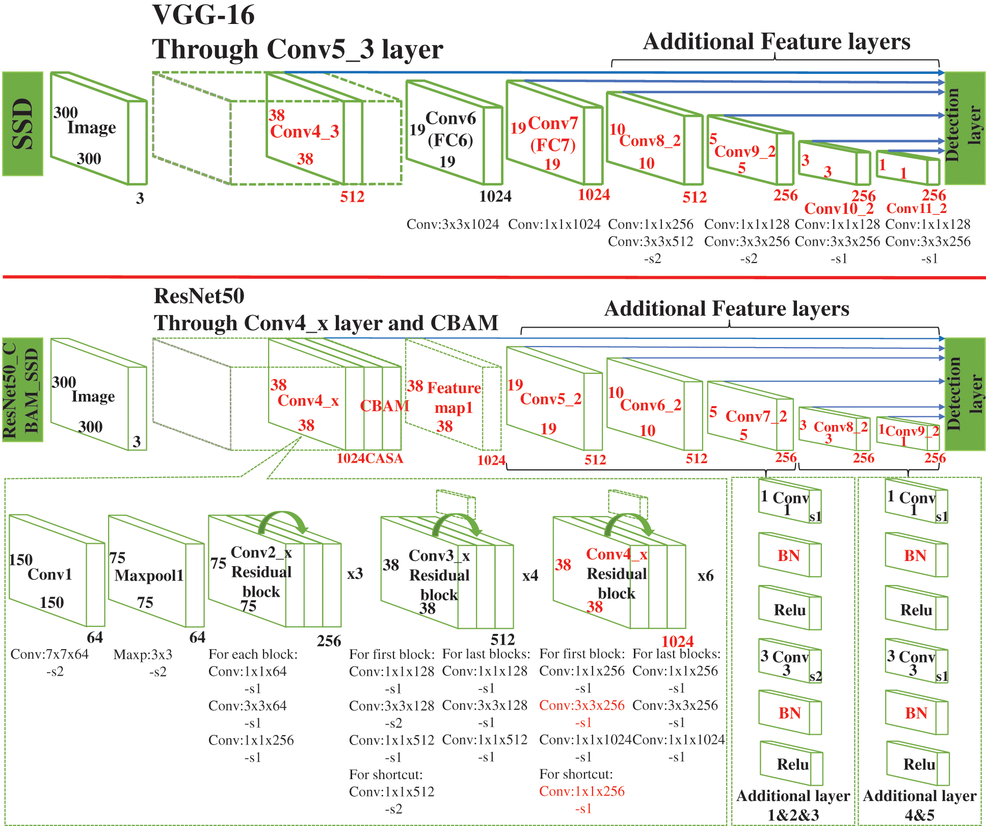
Figure 5: Comparison of SSD network with ResNet50_CBAM_SSD network

2.2 Saliency Detection Stage

2.2.1 Related Works

After obtaining the images of the four types of bolts, the bolts with marker lines (Bolt_A and Bolt_B) are selected as the next data set. For the subsequent accurate angle measurement of marker lines, saliency detection is used to achieve feature extraction of the marker line regions.

Saliency detection refers to the extraction of salient areas in an image by intelligent algorithms that simulate human visual characteristics. Zhao et al. [33] designed a new edge preservation loss that guides the network to learn more detailed information in boundary localization by integrating multi-level and multi-scale features; Song et al. [56] used a fully convolutional neural network to extract rich multilevel defect features and adopt the CWB and the residual decoder block (RDB) alternatively to integrate the spatial features of shallower layers; Qin et al. [58] similarly used a densely supervised encoder-decoder network and a residual optimization module for saliency prediction and saliency map optimization, respectively.

Saliency detection has a good performance in feature extraction of single objects. However, the direct usage of these existing saliency detection models does not accurately extract the marker regions due to the varying shapes of marker lines, low contrast and noise interference, as shown in Fig. 6.

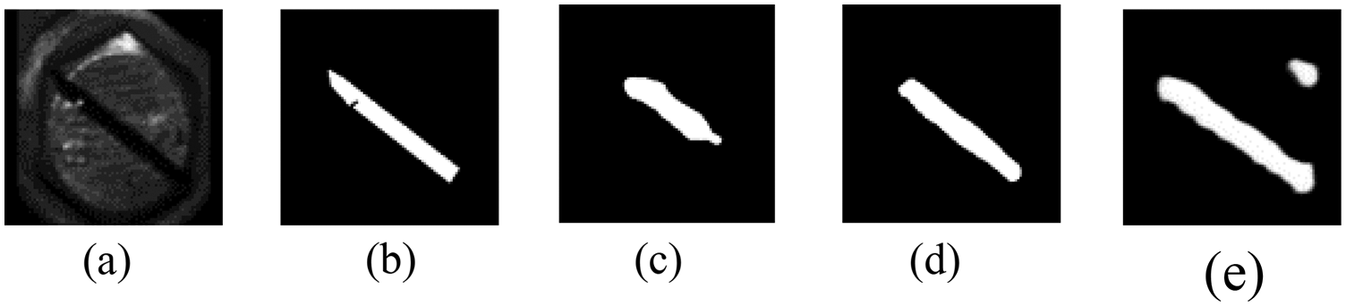
Figure 6: The marker line regions predicted by the existing saliency detection model. (a) Image (b) Ground-truth (c) PFA (d) EDR (e) BAS

2.2.2 A2-PFN

Based on the prediction results of several mainstream saliency detection networks currently available, the PFA with the highest evaluation metric score is selected as the base network architecture. However, there are two problems when using PFA to predict marker lines:

1.    The marker line boundaries are poorly extracted, and the obtained saliency regions tend to exceed the manually marked line areas. This is a fatal problem.

2.    Compared with other networks, which often have fatal cases where the predicted marker positions and angles deviate from the manually labeled positions, PFA rarely has similar cases (as shown in Fig. 6c), but still has deviations when the noise is high or when the contrast between foreground and background is low.

Accordingly, A2-PFN is proposed to solve the above two problems, and its network structure is shown in Fig. 7.

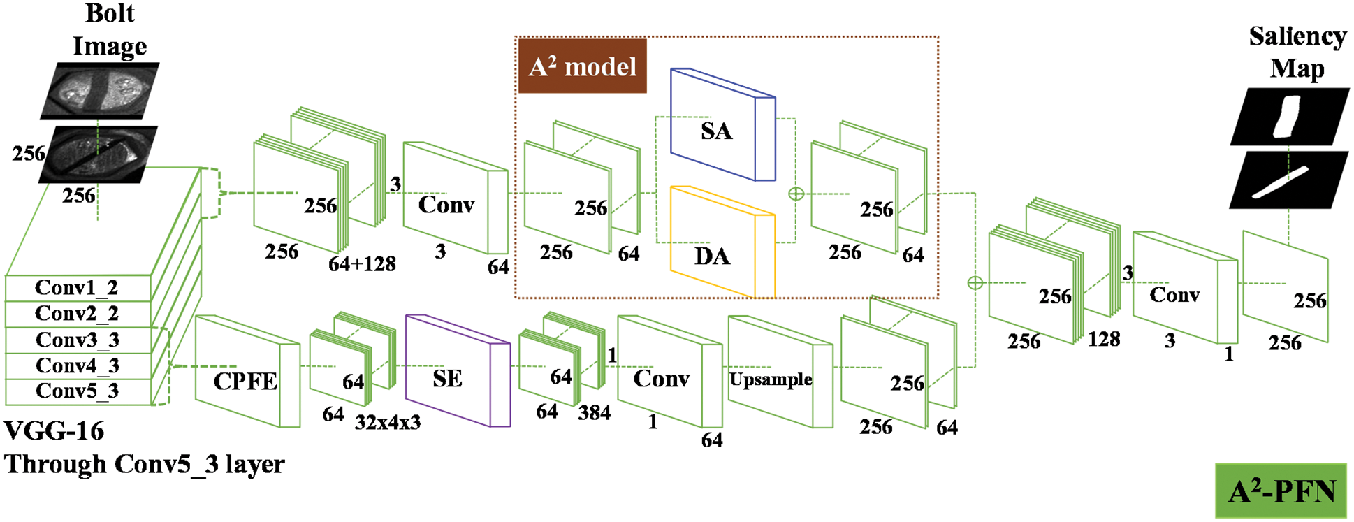
Figure 7: A2-PFN

Specifically, the bolt images are firstly fed into the VGG-16 network for initial feature extraction. The shallow networks, i.e., Conv1_2 and Conv2_2, are extracted, and the generated feature maps are passed through SA and DA to focus on the boundary features of the marked lines, respectively, and the features extracted from both are fused. Meanwhile, the deeper networks, i.e., Conv3_3 to Conv5_3, are extracted and the generated feature maps are passed through the Context-aware Pyramid Feature Extraction (CPFE) [33] module to fuse the initially extracted multi-scale features. SE is used to remove the weights of the noisy channels from the fused features, so that they focus more on the channels that are prominent in the marked line regions. Finally, the feature maps generated from the above two steps are combined and then compressed into a binary image by 3 × 3 convolutional layers, and this binary image is the extracted salient regions, i.e., marker lines.

The fusion of two attention mechanisms, i.e., SA and DA, is innovatively applied into the network to solve the problem of poor boundary feature extraction. The structure of SA is the same as that used in CBAM in the previous section. DA is structured by three 1 × 1 convolutional layers, respectively, with softmax layers added after the second and third convolutional layers. The global feature is obtained by bilinear pooling of the first and second layers, and the local feature under the global feature is obtained by multiplying global feature with the third layer by the corresponding matrix. The specific model is shown in Fig. 8.

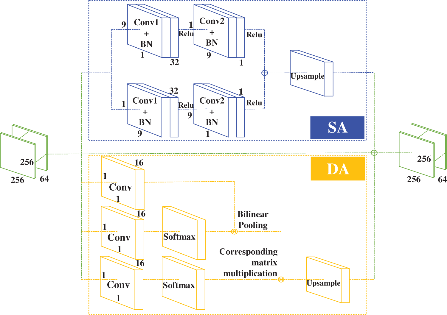
Figure 8: A2 model

The role of SA here is to focus on local features, just as the role of SA in CBAM. However, using SA to focus on local features only is prone to local optimal solutions, thus losing global feature information [35], which is why the predicted labeled line region exceeds the manually labeled marker line region. However, local information is indeed one of the important influencing factors for accurate extraction of boundary information, so DA that focuses on both global features and local features is adopted. Rather than directly replacing SA with DA, DA and SA are combined in parallel. This means that the shallow features extracted in the previous level are focused on local features through SA and on local information while focusing on global features through DA, respectively. Then the feature information obtained from both is fused to obtain the optimized local feature information, making it possible to predict the boundaries of the marked lines more accurately. The specific effect is shown in Fig. 9, and the enhancement effect brought by more accurate boundary extraction is shown in Fig. 10.

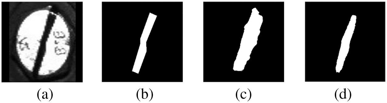
Figure 9: Comparison of predicted results (a) Image (b) Ground-truth (c) PFA (d) A2-PFN

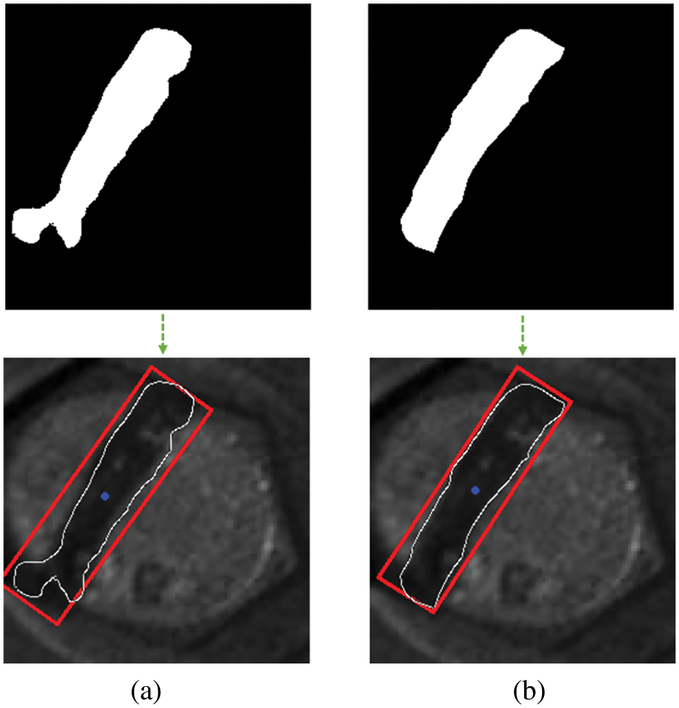
Figure 10: Comparison of the extraction results (a) PFA (b) A2-PFN

The outputs of Conv3_3 to Conv5_3 of the VGG-16 network are convolved through a 1 × 1 convolution layer and then convolved through three 3 × 3 voids with dilation rates of 3, 5, and 7, respectively. This is the structure of the CPFE module, and it is shown in Fig. 11.

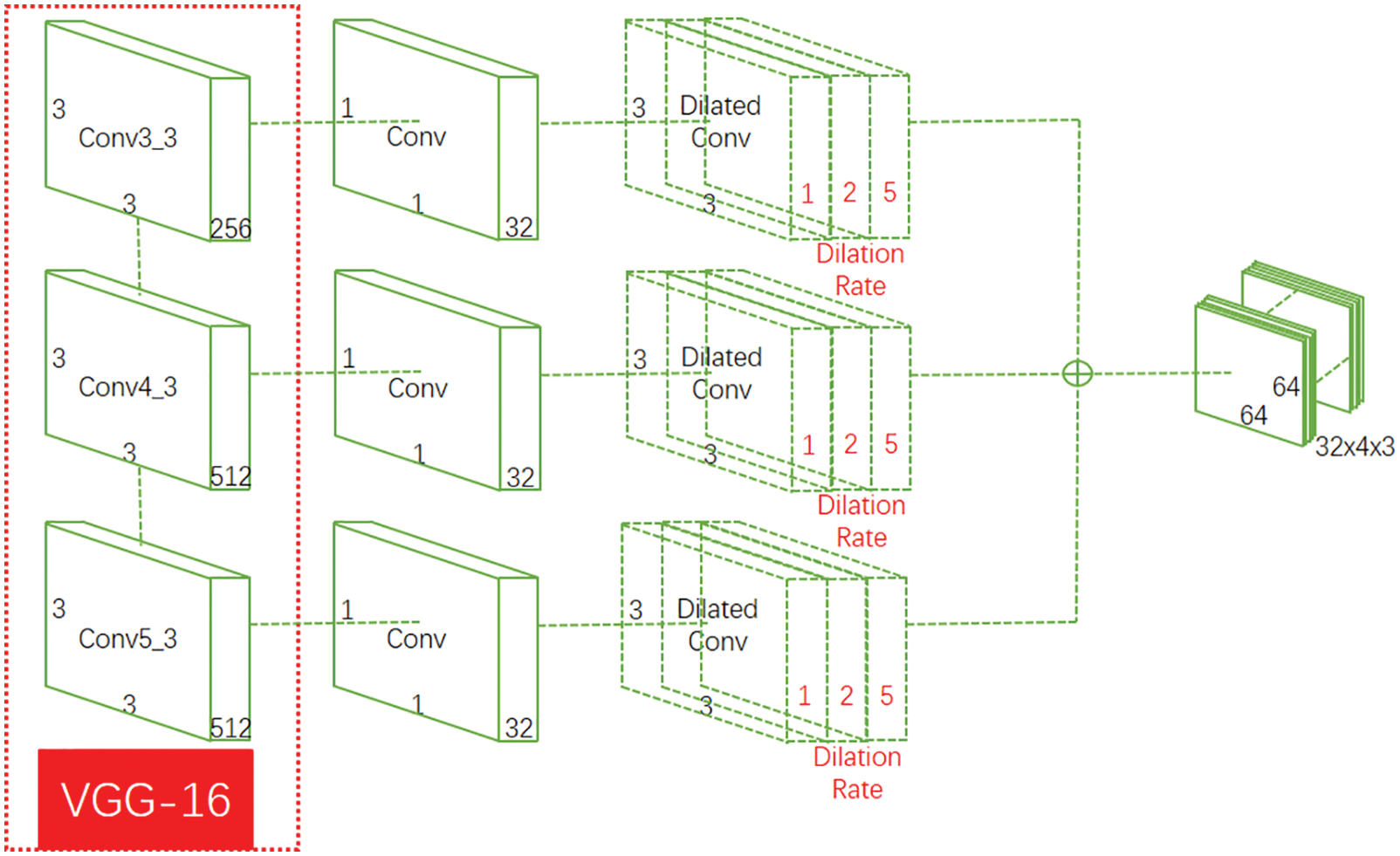
Figure 11: CPFE module

Inspired by Wang et al. [59], the selection of the appropriate dilation rate is a very important issue. If the dilation rate is “3, 5, 7” (settings in the PFA), it can avoid local information loss, i.e., gridding effect, but long-ranged information might not be relevant. Setting the dilation rate in “3, 5, 7” has an effect on large objects, but it is counterproductive for slender objects. The problematic image happens to have a slender marker line, so an unreasonable dilation rate setting may be the cause of the problem. “1, 2, 5” was finally considered to be the appropriate dilation rate through experiments (see Section 3.4.1 for details). In addition, since the second problem occurred very rarely, only the SE attention mechanism was employed to focus on the high-level location information. The structure of SE attention mechanism is shown in Fig. 12.

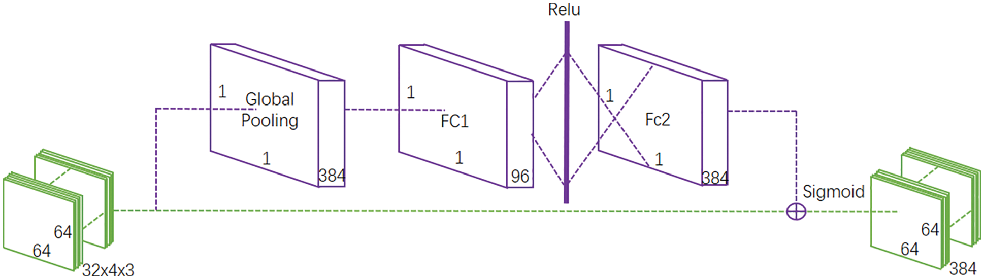
Figure 12: SE attention mechanism

2.3 Angle Calculation Stage

The general shapes of the marker line regions are classified as rectangular, but the shapes of the marker line regions may change due to wear and tear, resulting in different shapes of the marker line regions. If we only rely on the marker line regions extracted by saliency detection, it is difficult to have a uniform standard to judge the angular value of the marker line. Therefore, in this paper, after extracting the marker line regions in the previous stage, the marker line regions are further processed to obtain a method that can evaluate the marker lines generically, the rectangular approximation method, as shown in Fig. 13.

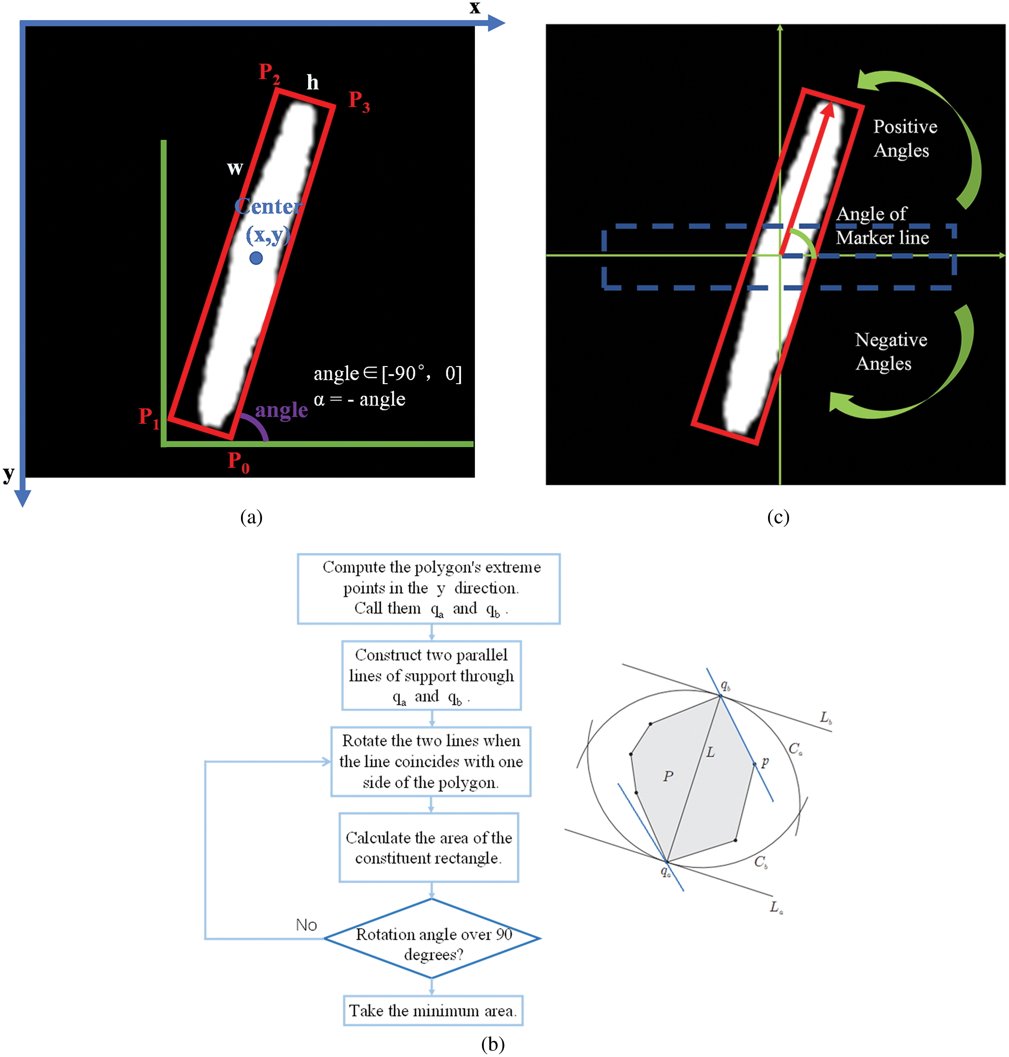
Figure 13: Schematic diagram of angle calculation

The method is described below:

1)   The edge features of the marker line are extracted and convex hull is constructed based on OpenCV to ensure the accuracy of the minimum rectangle extraction.

2)   The OpenCV-based rotating caliper algorithm is used to obtain the external rectangle with the smallest area and to obtain its center point coordinates (x, y), height (h), width (w), and initial rotation angle (angle). The specific algorithm flow is shown in Fig. 13b. Based on the fact that the origin of the OpenCV coordinate system is in the upper left corner, the counterclockwise rotation angle is negative and the clockwise rotation angle is positive with respect to the x-axis, so take α=−angle for calculation convenience. This initial rotation angle is the counterclockwise rotation of the horizontal axis (x-axis) with respect to the first edge of the encountered rectangle.

3)   In order to get the rectangular box on the saliency map, only the four parameters are not enough, the coordinates of the four endpoints of the rectangle are needed. As shown in Fig. 13a, the endpoint coordinates can be deduced from the trigonometric relationship, and the respective equations are shown below:

P0(x0,y0)={x0=x−12h⋅sin⁡(α)−12w⋅cos⁡(α)y0=y+12h⋅cos⁡(α)−12w⋅sin⁡(α)(3)

P1(x1,y1)={x1=x+12h⋅sin⁡(α)−12w⋅cos⁡(α)y1=y−12h⋅cos⁡(α)−12w⋅sin⁡(α)(4)

P2(x2,y2)={x2=2x−x0y2=2y−y0(5)

P3(x3,y3)={x3=2x−x1y3=2y−y1(6)

4)   The deviation angles of the upper and lower edges from the horizontal line are calculated based on the coordinates of each of the four vertices. The horizontal position is the horizontal line and the vertical position is the normal line, the deviation to counterclockwise is positive and to clockwise is negative from the horizontal position.

5)   Take the average of the two angles as the angle of deviation from the horizontal position of the marker line, and make an arrow at the center point to indicate. The angle of marker line is shown in Fig. 13c.

The angles calculated by the rectangular approximation method for each marker line are summarized and plotted in an angle table.

3  Experiments and Results

3.1 Datasets and Training Process

3.1.1 Datasets Collection

In order to achieve high-definition image detection of train vehicles, this paper adopts a new 360° dynamic image detection system for the whole train vehicle to obtain 360° high-definition images of the whole vehicle status. This system has the advantages of high detection efficiency, high automation and high image recognition. The system is designed with 10 sets of integrated image acquisition modules to provide full coverage of the roof, sides, windows and under walkway sections of the vehicle. Each integrated image acquisition module consists of a line array camera and a non-visible infrared laser light source, forming an enclosed, IP67 rated integrated module, as shown in Fig. 14. The LQ camera module is mainly used to scan the underbody and side walk sections of the vehicle, and can collect the data set applicable to this paper. The camera used in this paper is a 4 K HD camera with image resolution up to 1mm/pixel, which supports multi-level magnification for small parts and can clearly view the marker lines of bolts.

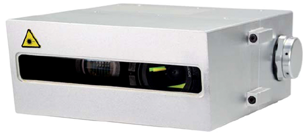
Figure 14: LQ camera module for integrated acquisition

Each integrated image acquisition module in the system is installed in the central bed position of the rail track, both sides of the rail and above the side, forming a complete circle layout from top to bottom, which can be seen Figs. 15a and 15b for installation method. 10 groups of image acquisition modules in the system are responsible for scanning and processing vehicle images within a certain angle range, and finally synthesize high-definition images through feature point positioning image stitching technology, as shown in Fig. 15c.

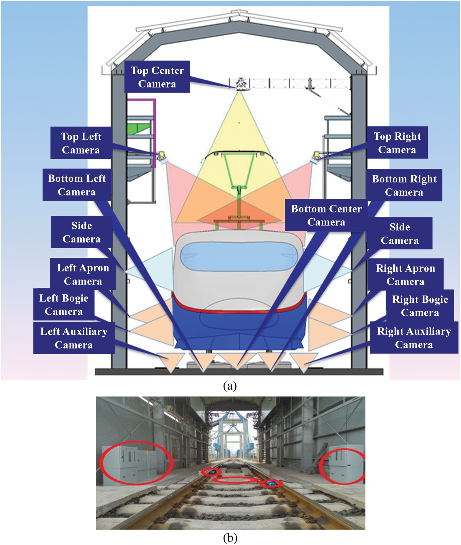
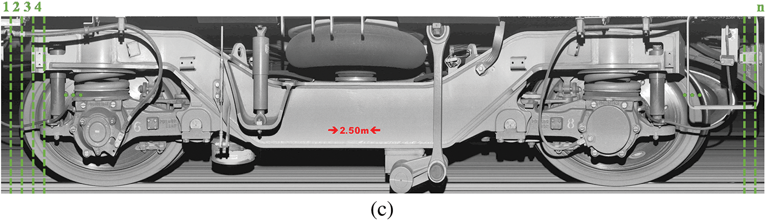
Figure 15: Acquisition of Original Datasets (a) Schematic diagram of the image acquisition unit (b) Field inspection unit (underneath the vehicle) (c) Composited high resolution image of the bogie side travel section

3.1.2 Overall Training Process

All deep learning networks in this paper are trained, validated, and tested using NVIDIA GeForce RTX 2060, and the code framework is pytorch1.5. The overall training process is shown in Fig. 16, which is described as follows.

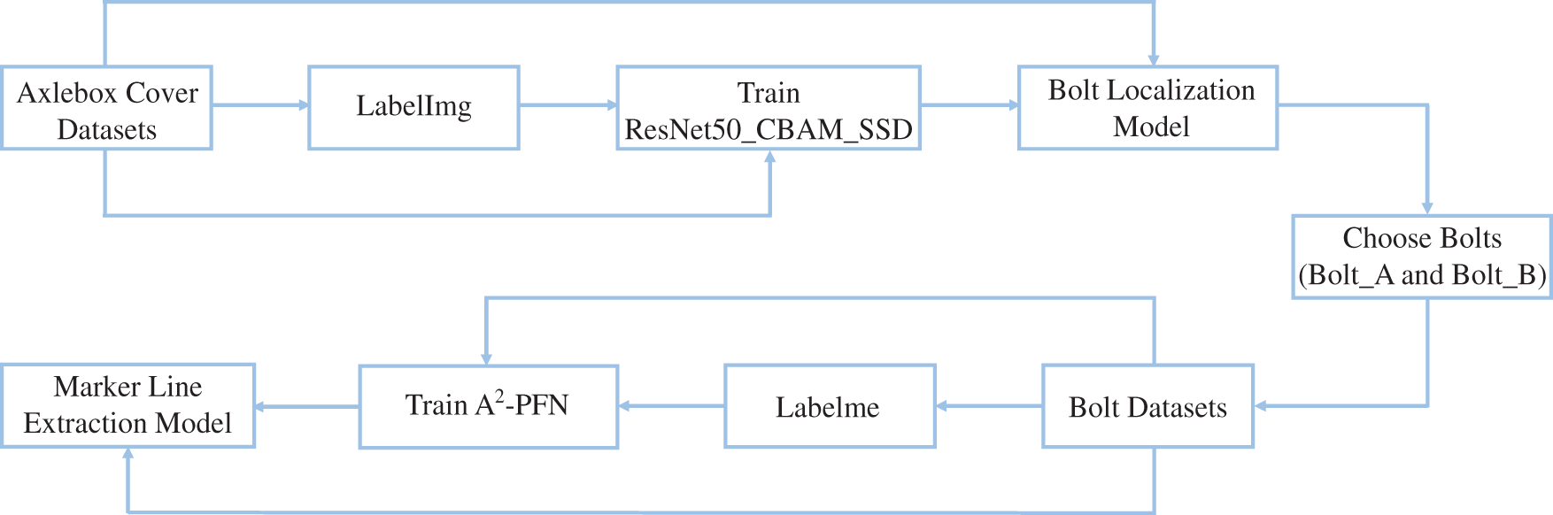
Figure 16: Overall training process

Step 1: LabelImg is used to mark four kinds of bolts from the axlebox images, and they are applied to train the ResNet50_CBAM_SSD for the bolt localization.

Step 2: Labelme is used to mark the marker line regions of Bolt_A and Bolt_B, and they are applied to train the A2-PFN for extracting the saliency regions of marker lines.

3.2 Dataset Labeling

3.2.1 Labeling for Object Detection

Since the object detection model used in this paper is a supervised model, four different bolt regions must be labeled to make the network more focused on the location of the target criteria box before model training. At present, most datasets are manually labeled [53], and some small errors due to manual labeling are not taken into account in this paper.

Currently, labelImg is commonly used in the field of object detection to manually label target criteria box. Firstly, enter the axlebox cover data set into labelImg and select the PascolVoc format. Secondly, the standard frame of the bolt is manually labeled on the image and the label names are labeled as “Bolt_A”, “Bolt_B”, “Bolt_C”, “Bolt_D” according to the characteristics of the bolt. Finally, the manually labeled file in “.xml” format is saved and this file will be used for supervised model training. The specific method of manually labeling images with labelImg is shown in Fig. 17.

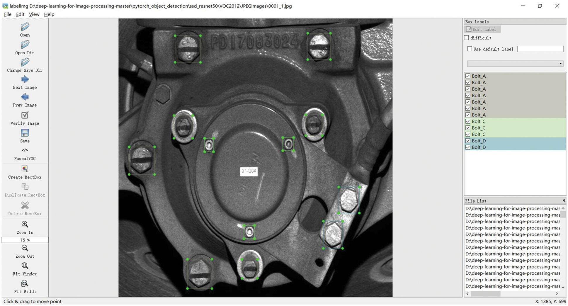
Figure 17: Label image for object detection

3.2.2 Labeling for Saliency Detection

Similar to the use of labelImg to label the object detection dataset, labelme is usually used to manually label the ground-truth in the field of saliency detection. Firstly, the bolt dataset is entered into labelme. Secondly, frame the marker line region along its edges on the image, getting as close to the edges as possible in the process, and change its label name to “marker line”. Finally, save the manually labeled file in “.json” format and convert the “.json” file into a “.jpg” file by means of a command. This “.jpg file”, i.e., the ground-truth, will be used for supervised training of the saliency detection model. The specific method of manually framing out the ground-truth with labelme is shown in Fig. 18.

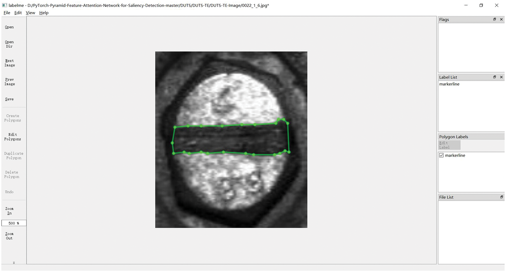
Figure 18: Label image for saliency detection

3.3 Bolt Localization

3.3.1 Object Detection

In this paper, experiments are conducted on the axlebox cover dataset to verify the effect of the ResNet50_CBAM_SSD. There are 370 images in the axlebox cover dataset, including 266 images in the training set, 67 images in the validation set, and 37 images in the test set.

In the dataset of axlebox cover, four different classes of bolts are marker, where Bolt_A and Bolt_B are bolts with marker lines and Bolt_C and Bolt_D are bolts without marker lines. The input size is 300 × 300 × 3, the batchsize is set to 2, and the learning rate is reduced from 0.0005 to 0.000045. The dataset in this paper is in PASCAL VOC 2012 format, and the training generated Eval mAP is the default evaluation metric for this class of dataset. The loss function change vs. learning rate change and mAP curves during training are shown in Fig. 19.

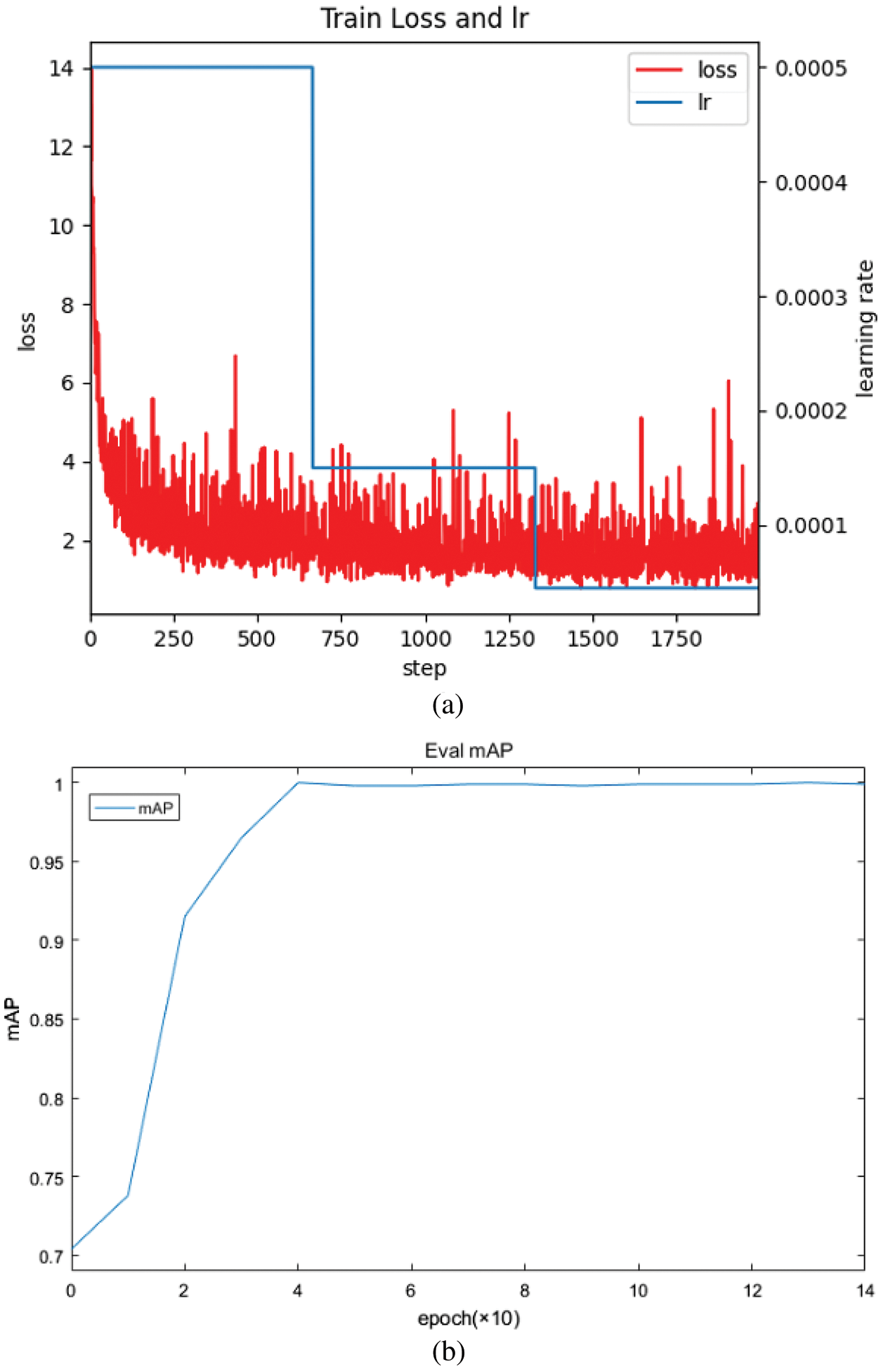
Figure 19: The results of training (a) Convergence curve of the training process of ResNet50_CBAM_SSD (b) Curve of eval mAP

In this paper, we compare ResNet50_CBAM_SSD with SSD and ResNet50_SSD, and the statistical results are shown in Table 1. When the uniform input image size is 300 × 300 × 3, although there are more parameters than ResNet50_SSD, it is much more streamlined than SSD, and the detection accuracy (mAP(IoU = 0.5), mAP(IoU = 0.5:0.95)) and FPS have significant accuracy improvement as well as detection speed improvement compared with the previous model. The mAP (IoU = 0.5:0.95) is 2.4% higher than SSD, 1.4% higher than ResNet50_SSD, and the FPS is 5 higher than SSD and the same as ResNet50_SSD.

A comparison of the recognition accuracy of the four types of bolts is shown in Table 2. In order to analyze the results more clearly and comprehensively, a compromise IoU of 0.75 is chosen. ResNet50_CBAM_SSD made the biggest improvement in the small target detection, i.e., Bolt_C metric, rising from 0.202 to 0.586, for a total increase of 0.384, mainly due to the adoption of ResNet50 to replace VGG-16. In addition, the important Bolt_A and Bolt_B rose from 0.973 to 0.983 and from 0.683 to 0.75, respectively, improving the accuracy even more. The overall mAP also rose from 0.654 to 0.77, for a total increase of 0.116. In terms of accuracy data, ResNet50_CBAM_SSD effectively improves the reliability and accuracy of the model.

It is one-sided to judge model strengths and weaknesses only at the data level, so a comparison between actual detection results is also necessary. A comparison of the detection accuracy of three models is shown in Fig. 20. It is easy to find that ResNet50_CBAM_SSD is faster in terms of accuracy convergence compared to SSD than ResNet50_SSD, and the final accuracy of ResNet50_CBAM_SSD is relatively higher (when IoU = 0.5). In addition, when IoU = 0.5:0.95, ResNet50_CBAM_SSD achieved higher accuracy relative to the other two.

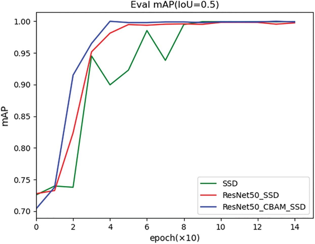
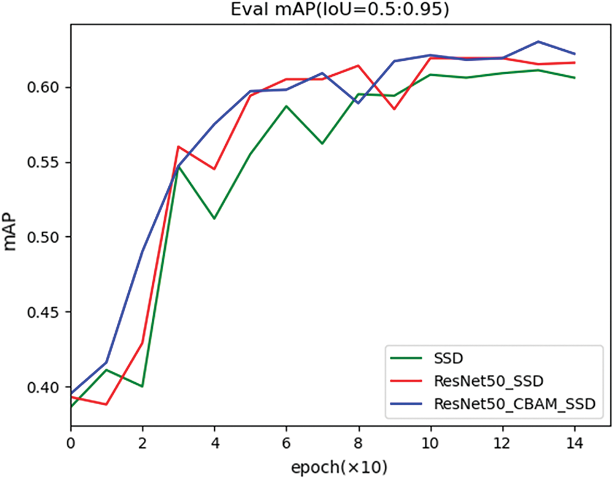
Figure 20: Comparison of the detection accuracy of three models during training

Besides, a comparison of results of three models is shown in Fig. 21. It can be visualized that the SSD algorithm can detect the bolts with marker lines, but ignore the small bolts (Bolt_C). ResNet50_SSD algorithm can achieve the detection of part of the small bolts, but will be missing and lose some important bolts with marker lines (Bolt_B). The improved ResNet50_CBAM_SSD algorithm in this paper can correctly detect most of the bolts.

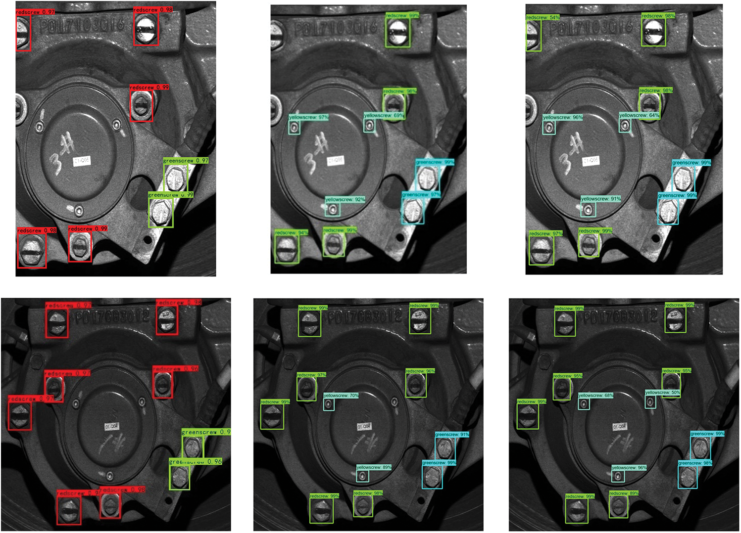
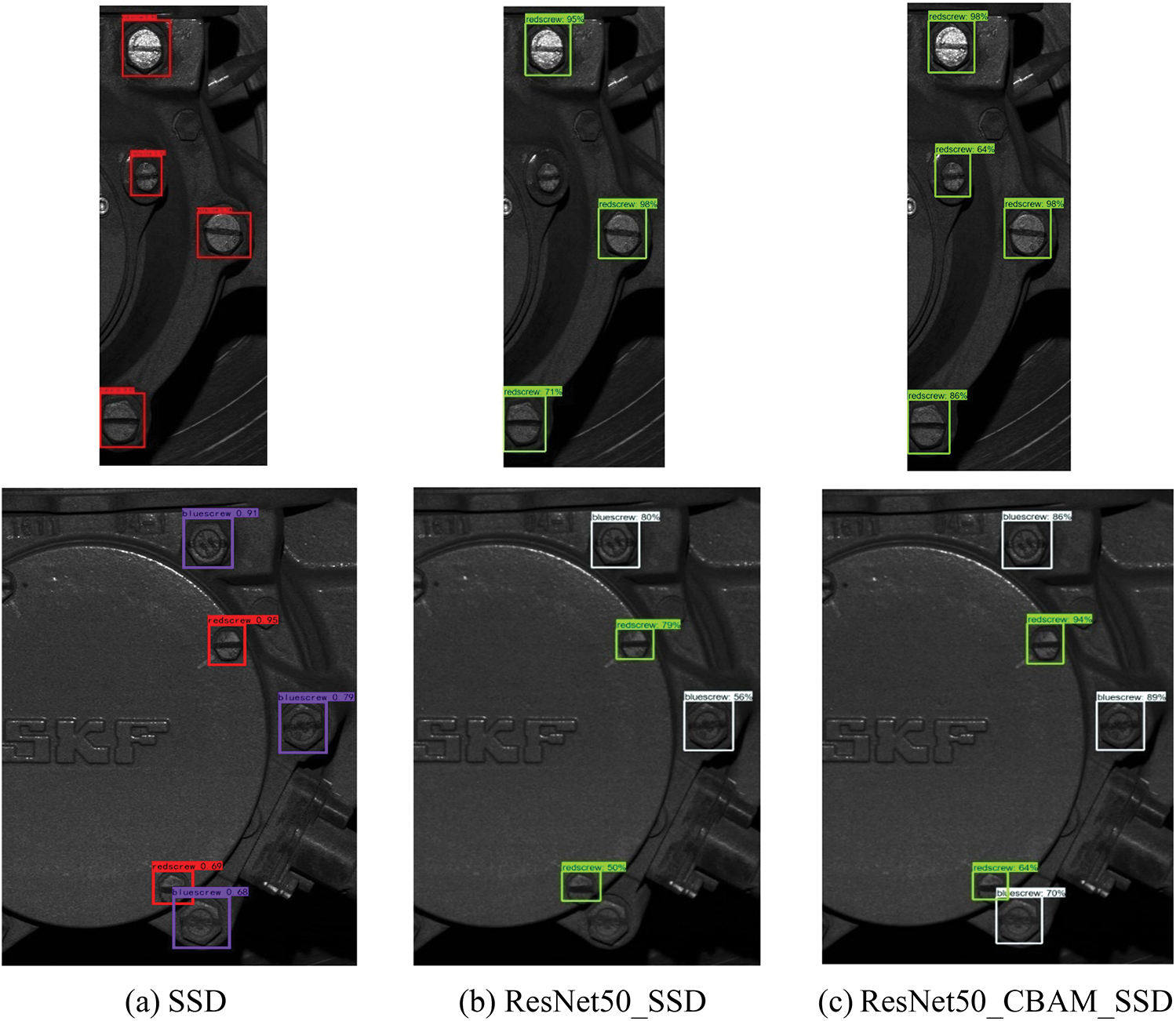
Figure 21: Comparison of results of three models

3.3.2 Visual Explanation

The current deep learning models work well but are poorly interpretable because the CNN model is a black box [60]. In this paper, Grad-CAM++ [61] is introduced to obtain the feature attention heat map of the last layer of the feature extraction layer in order to verify whether the attention mechanism incorporated in this paper has any effect on the overall model.

Compared with Grad-CAM [60], Grad-CAM++ is more advantageous for multi-objective heat map acquisition, and the accuracy will be a bit higher. The bolt inspection of the axle box cover is indeed a multi-objective inspection, so the Grad-CAM++ method was finally chosen.

The obtained heat maps are shown in Fig. 22. It is clear to see that the addition of the attention mechanism results in a larger sensory field and the ability to focus on more important bolt features.

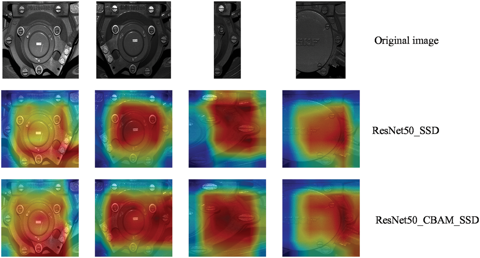
Figure 22: Comparison of feature visualization before and after adding the attention mechanism

3.4 Marker Line Extraction

3.4.1 Hyperparameter Configuration

For the saliency detection part, several parameters with deeper influence have been adjusted during training the model, such as dilation rate, initial learning rate and epochs. The dilation rates are chosen to be “3,4,7” and “1,2,5”. Appropriate dilation rates can effectively reduce the loss and perform better in terms of indicators. The initial learning rate is also closely related to the update of the weight parameters. The larger the initial learning rate, the larger the loss will be, and the faster the network diverges, making it more difficult to converge. In addition, choosing appropriate epochs can improve the running speed of network and let the model converge properly. The batch size is uniformly set to 10, which is the maximum this GPU can handle. In addition, the Adam optimizer was chosen for the optimizer. The experiment results are shown in Table 3 below.

By comparing the training loss and validation loss, precision, recall and MAE, we can initially find that when the dilation rate is set to “1, 2, 5”, epochs are set to 200, and initial learning rate is set to 0.0001, the performance of each indicator is the best. After reviewing the related metrics of each epoch, we finally found that the best metrics are achieved when epochs are set to 150. Therefore, the final setting of epochs for this experiment is 150.

3.4.2 Saliency Detection

From the above detected bolts, the bolts with marker lines (Bolt_A and Bolt_B) are selected by label category and combined into a new dataset to be substituted into the A2-PFN for saliency detection and extraction of marker line regions. In the experiment, a total of 1756 images of bolts with marker lines are resized into 256 × 256 × 3 images, which are assigned to the training set, validation set and test set in the ratio of 8:1:1. The batch size is set to 10, the initial learning rate is set to 0.0001, the epochs are set to 150, and the dilation rate is set to “1,2,5”. In addition, the Adam optimizer is chosen for the optimizer. However, we do not consider the learning rate decay, because using this strategy would cause the training error to rise. The loss curve of the training process is shown in Fig. 23.

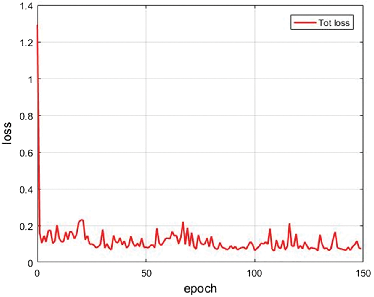
Figure 23: Curve of training loss of A2-PFN

The trained best weights can be obtained to characterize the marker line region of any axle box cover bolt, and a qualitative comparison of our results with those of PFA [33], EDR [56], BAS [58], U-2 [62], PoolNet [63], and BASv2 is shown in Fig. 24.

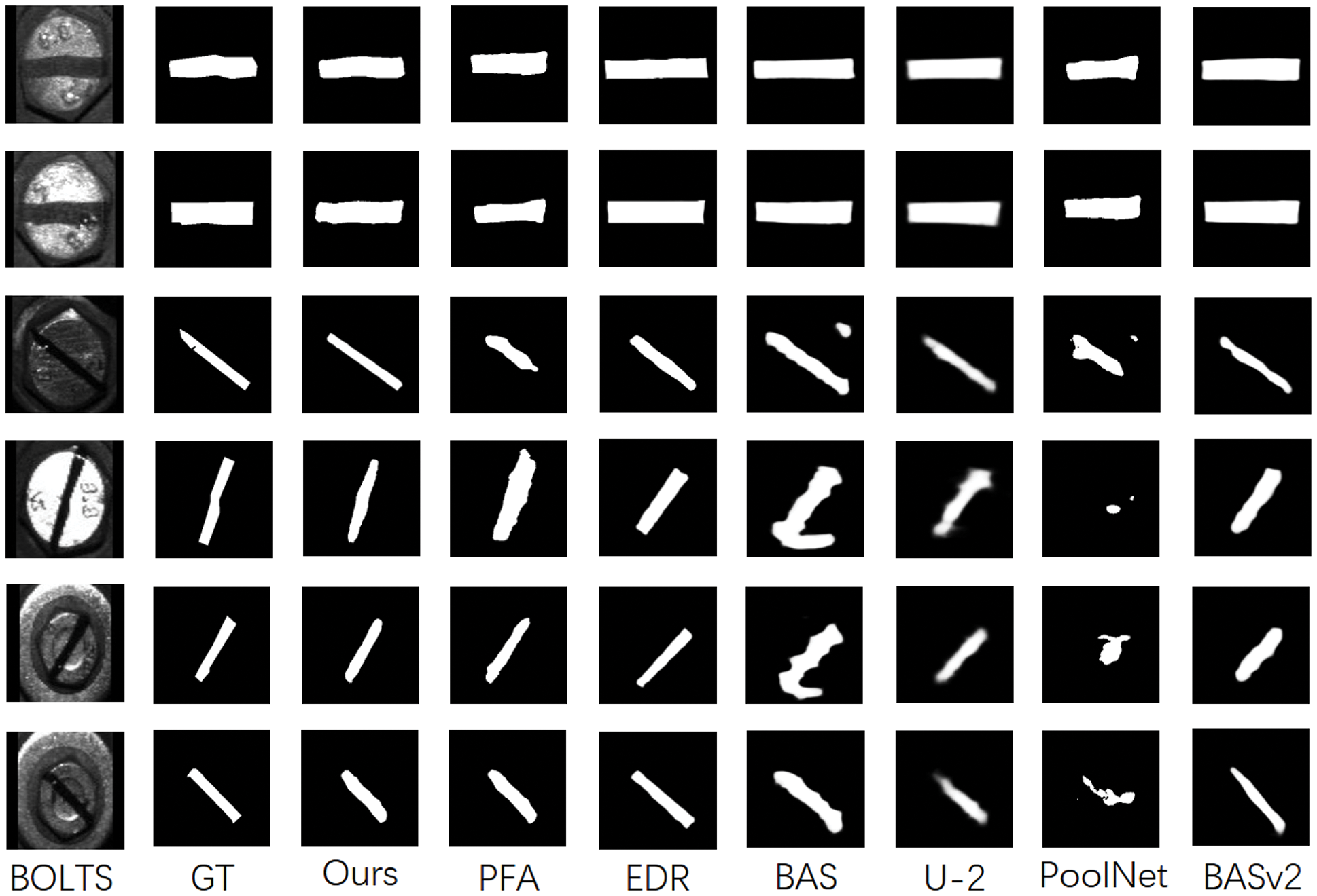
Figure 24: Qualitative comparison of the results of feature extraction of the marker lines of the bolts

From the qualitative comparison of each model in Fig. 24, it can be found that the results obtained from each model differ little from the ground-truth when the marker lines are located above and below the horizontal position. However, when the marker lines are skewed, the BAS, U-2, and PoolNet models fail to correctly identify the marker line regions. The PFA, EDR, and BASv2 are able to extract saliency regions similar to the marker line region, but with a skewed angle. Our method is able to get closer to the ground-truth and ensure that the angle does not deviate too much. In addition, for slender marker lines, such as the examples in the third and fourth rows, our method is able to extract the saliency of the marker lines without exceeding the ground-truth too much, while the other methods obviously inflate the saliency region too much beyond the ground-truth due to unreasonable parameter settings.

In order to compare our model with other advanced models from a quantitative perspective, we introduced four metrics, which are calculated as described below:

precision=TPTP+FP(7)

recall=TPTP+FN(8)

MAE=1W×H∑pW×H|S(p)−GT(p)|(9)

Fβ=(1+β2)×Precision×Recallβ2×Precision+Recall(10)

Precision and recall are calculated as shown in Eqs. (7) and (8), where TP indicates a positive case is correctly classified as a positive case, FP indicates a negative case is incorrectly classified as a positive case, and FN indicates a positive case is incorrectly classified as a negative case. The curve consisting of precision and recall can determine the good or bad performance of the model, and the closer the curve is to the upper right corner, the better the performance of the model. Based on the P-R curve of the test set during the training process, the model can be judged to have a better performance. In addition, we used three metrics, mean absolute error (MAE), F-measure (Fβ) [53], and area under the receiver operating characteristic curve (AUC), to measure the performance in a comprehensive manner. The MAE is calculated as shown in Eq. (9), where refers to the saliency map, GT(p)refers to the ground-truth (GT), while W and H are the width and height of the image, respectively. The result of MAE measures the difference between the ground-truth and the saliency map at the pixel level, and the closer the MAE is to 0, the less the difference is. Fβ is calculated as shown in Eq. (10), and according to what is stated in [53], here β2=0.3, which measures the accuracy, the closer Fβ is to 1 indicates the higher accuracy. AUC is the area under the receiver operating characteristic curve, and the closer the AUC is to 1 the better the model performance.

The values of specific quantitative metrics are shown in Table 4, and a quantitative comparison of the results of feature extraction of the marker lines of the bolts is shown in Fig. 25.

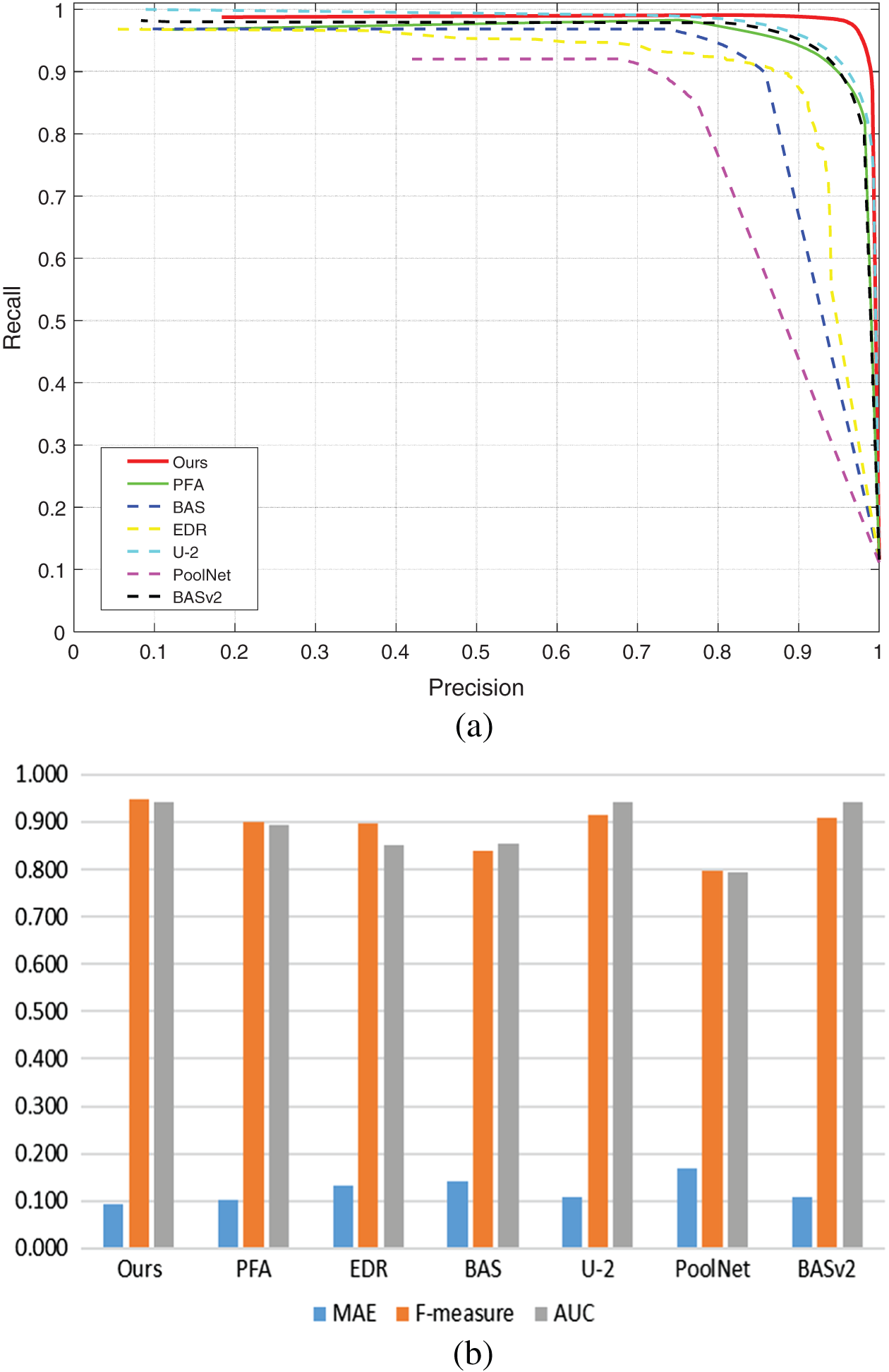
Figure 25: Quantitative comparison of the results of feature extraction of the marker lines of the bolts (a) P-R curve (b) MAE & F-measure & AUC

According to Table 4, the MAE of our method is the smallest among the compared methods, reaching 0.092, which is 0.012 lower than the lowest PFA. In addition, Fβ and AUC reach the highest values among the compared methods, with 0.948 and 0.943, respectively. Finally, according to the P-R curves in Fig. 25, the curve of our method is closer to the upper right corner than the curves of the other methods and can mostly wraps around the curves of the other methods. According to the results shown above it is proved that our model has better performance.

Since the features located above and below the horizontal position in the marker line dataset are generally simpler and far more numerous than in other cases, the overall difference in the effectiveness of more advanced deep learning-based saliency detection of such marker lines is not significant. However, for angularly skewed marker lines with little data, the network detects very different saliency regions. Our method, the A2-PFN, is able to perform the task of detecting such bolts because it extracts feature regions that do not produce too much deformation and fit more closely to the saliency regions in the original figure, while not exceeding the ground-truth too much when dealing with slender marker lines, as illustrated by the P-R curves calculated in Fig. 25. Likewise, the error (MAE) and accuracy (F-measure and AUC) are better as a result according to Table 4.

3.4.3 Visual Explanation

Similar to what has done in Section 3.3.2, Grad-CAM++ [61] is also used to visualize the feature heat map for the A2 model. It can be clearly seen in Fig. 26 that the addition of the attention mechanism makes the model pay more attention to the area around the marker lines and reduces a certain amount of background noise interference.

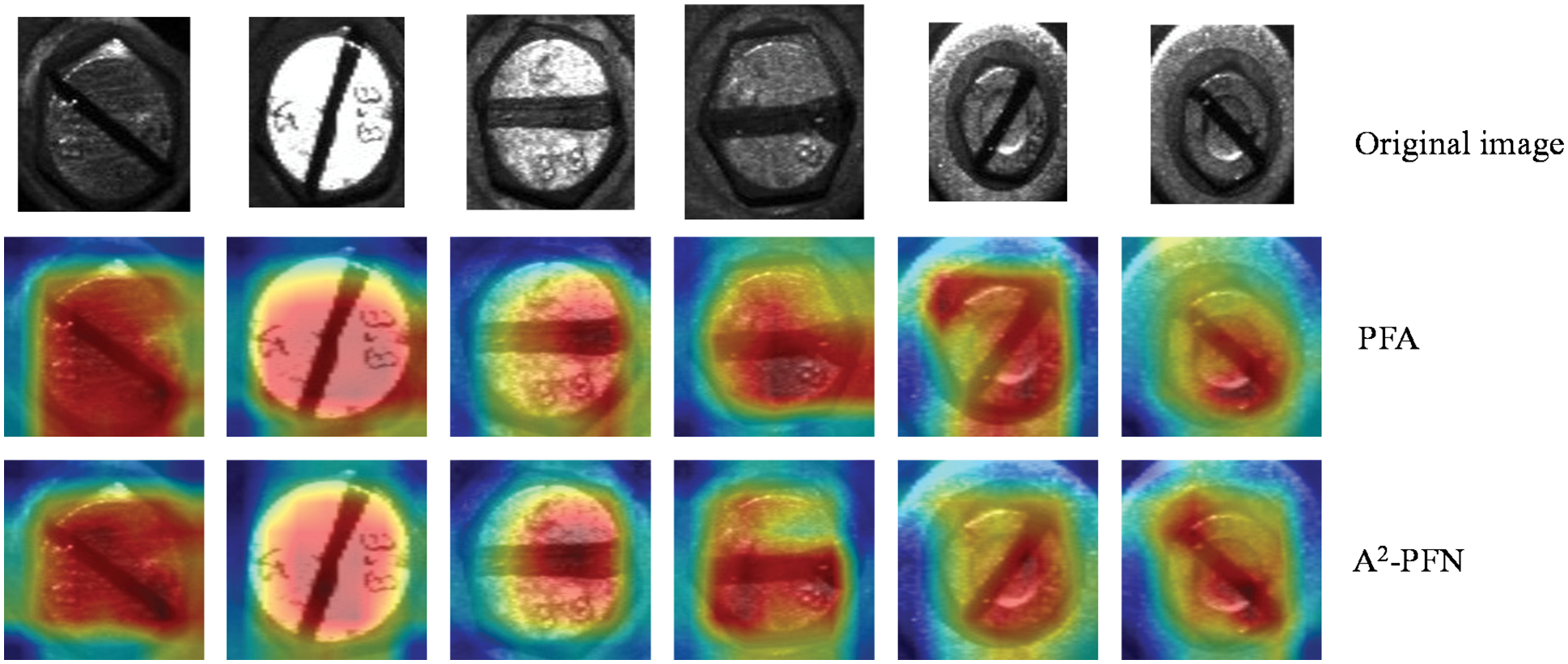
Figure 26: Comparison of feature visualization before and after adding the attention mechanism

3.4.4 Comparison of Prediction Efficiency

In practical applications, the prediction efficiency of the algorithm is also one of the criteria for judging a model. If the prediction efficiency is too slow, it is difficult to be applied directly in practice. Hence, FPS is also used in this work to achieve the comparison of prediction efficiency. Similarly, the FPS results of our method are compared with those of PFA, EDR, BAS, U-2, PoolNet and BASv2, and the results are shown in Table 5.

Although PFA achieved the highest FPS of 59.1, A2-PFN still achieved the second highest FPS of 56.8, with an FPS reduction of 2.3. Taking into account that A2-PFN is higher than PFA in all accuracy metrics, we believe that a 2.3 reduction in FPS is acceptable. In addition, the FPS of A2-PFN is still much higher than the other methods, where it is 14.2 FPS higher than the third-ranked BAS and 18.6 FPS higher than the fourth-ranked BASv2. This indicates that A2-PFN still has a great advantage in FPS and accuracy when used for marker line detection.

3.5 Angle Calculation

After the extraction of the features of marker lines, this paper introduces the angle table as an evaluation index to evaluate the angle measurement of the marker line. Based on the best weights obtained from the previous stage, feature regions of 1756 marker lines are generated, and the angle table is drawn by using MATLAB and according to the angle measurement method specified in Chapter II, Section 2.3. The angle measurement process according to the rectangular approximation method of all the marker lines is shown in Fig. 27.

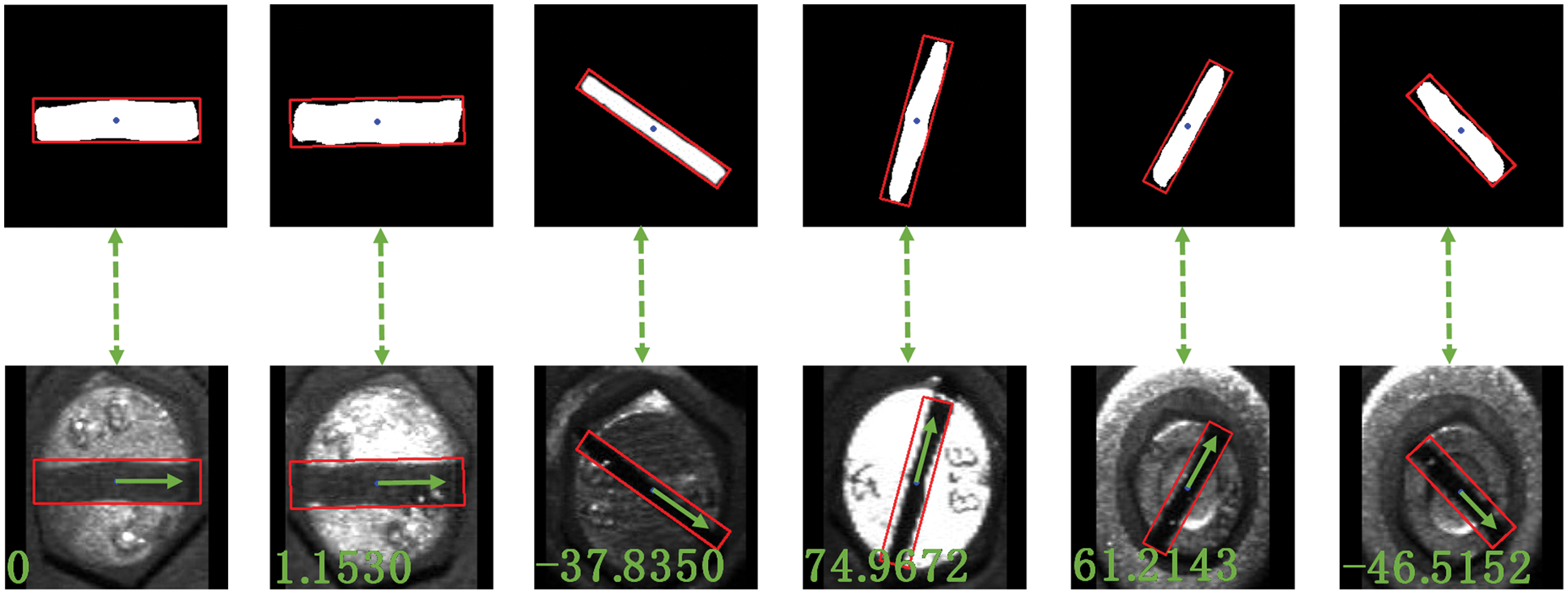
Figure 27: Angle measurement process of marker lines based on rectangular approximation method

Theoretically, the bolt tension is sufficient to keep the bolt tight only when the marker line is in the horizontal position (0°). However, out of 1756 angles of the marker line finally calculated by the method of this work, only 104 angles were 0°. In fact, judging from the work experience of subway maintenance personnel, a large number of marker lines that deviate from 0° by only a few degrees are still judged to be tight during routine maintenance. This is due to a series of errors caused by the wear and tear of the marker lines, the failure to extract 100% of the entire marker lines during saliency detection, and the calculation of the minimum outer rectangle. After consultating with the metro maintenance staff, a suitable interval by their work experience is defined to judge the rotational looseness based on the angle of the marking line: an angle between ±5° is tight, an angle between ±5° to ±30° is loose, and an angle between ±30° to ±90° is severely loose.

In Fig. 28, 676 angles are included as samples and are plotted in an angle table. A coordinate point on the X-Y axis represents a marker line of a bolt, and the Z axis represents the value of its angle. According to the suitable regulations given above, i.e., the bolt with the risk of severely loosening is marked as red when the marker line deviates from ±30° to ±90°; the bolt with the risk of loosening is marked as blue when the marker line deviates from ±30° to ±5°; and the bolt with the risk of tightening is marked as green when the marker line deviates within ±5°. Among these 676 samples, a total of 60 bolts are marked red, 69 bolts are marked blue, and 547 bolts are marked green.

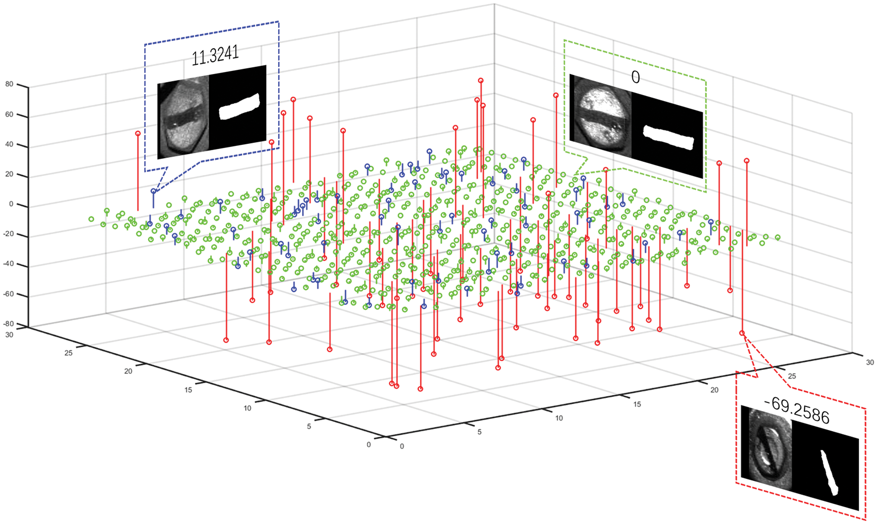
Figure 28: Angle table of the marker lines of the bolts

4  Conclusion

In this paper, we propose a system for measuring the angles of the marker lines of the bolts on axlebox cover of urban train vehicles based on deep learning, which mainly includes a ResNet50_CBAM_SSD network for object localization, A2-PFN based saliency detection for marker line extraction, a rectangular approximation method for measuring the angle of a marker line, and an angle table method to determine the bolt looseness by the angles.

1.    In the object localization stage, by comparing our proposed ResNet50_CBAM_SSD improved for the bolt features with the network before the improvement, our method can extract most of the four types of bolts more completely and effectively, where our mAP(IoU = 0.75) reaches 0.77 and fps reaches 16.6.

2.    In the saliency detection stage, A2-PFN is proposed to extract the marker line region closer to the ground-truth region, and the results are compared qualitatively and quantitatively with other state-of-the-art networks, and our results are better than the others, where our MAE reaches 0.092, F-measure reaches 0.948 and AUC reaches 0.943.

3.    In the angle calculation stage, the rectangle approximation method is used to create a regular rectangle that fits the marker line, and the angle of the marker line is calculated by averaging the angles of the upper and lower sides separately, and the angle size is used to determine whether the bolt is at risk of loosening. Ultimately, out of 676 bolt samples, a total of 60 bolts are loose, 69 bolts are at risk of loosening, and 547 bolts are tightened.

In summary, although the final results are able to meet the expectations of this paper, they still suggest some further improvements.

1.    The SSD network was first proposed in 2016, and more novel object localization networks have been proposed recently, such as YOLOv5. Using more novel networks and improving them for the data features, the results may be more desirable than those in this paper.

2.    It is hoped that in the future, it will not only be measured from the angle of image measurement, but also combined with other methods, such as ultrasonic detection, so as to truly achieve error-free detection of bolt loosening.

3.    This paper is mainly based on the Fault Detection and Diagnosis (FDD) technique and is missing the incipient fault detection and diagnosis (IFDD). As stated in [64], IFDD is very different from FDD, and IFDD has its unique superiority. It is hoped that IFDD-based bolt loosening detection can be added in the future.

Data Availability:The data used to support the findings of this study are available from the corresponding author upon request.

Funding Statement:This work was supported by the National Natural Science Foundation of China (Nos. 51975347, 51907117, and 12004240) and Shanghai Science and Technology Program (No. 22010501600).

Conflicts of Interest: The authors declare that they have no conflicts of interest to report regarding the present study.

References

 1.  Overview of Urban Rail Transit Lines in Mainland China in 2021. China Urban Rail Transit Association. https://www.camet.org.cn/xxfb/8658. [Google Scholar]

 2.  Zhou, D. H., Ji, H. Q., He, X. (2018). Fault diagnosis technology of high-speed train information control system. Journal of Automation, 44(7), 1153–1164. [Google Scholar]

 3.  Marino, F., Distante, A., Mazzeo, P. L., Stella, E. (2007). A real-time visual inspection system for railway maintenance: Automatic hexagonal-headed bolts detection. IEEE Transactions on Systems, Man & Cybernetics: Part C (Applications & Reviews), 37(3), 418–428. DOI 10.1109/TSMCC.2007.893278. [Google Scholar] [CrossRef]

 4.  Teloli, R., Silva, S. D., Ritto, T. G., Chevallier, G. (2021). Bayesian model identification of higher-order frequency response functions for structures assembled by bolted joints. Mechanical Systems and Signal Processing, 151, 107333. DOI 10.1016/j.ymssp.2020.107333. [Google Scholar] [CrossRef]

 5.  Jamia, N., Jalali, H., Taghipour, J., Friswell, M. I., Khodaparast, H. H. (2021). An equivalent model of a nonlinear bolted flange joint. Mechanical Systems and Signal Processing, 153(25–26), 107507. DOI 10.1016/j.ymssp.2020.107507. [Google Scholar] [CrossRef]

 6.  Lin, Q., Zhao, Y., Sun, Q., Chen, K. (2022). Reliability evaluation method of anti-loosening performance of bolted joints. Mechanical Systems and Signal Processing, 162(5), 108067. DOI 10.1016/j.ymssp.2021.108067. [Google Scholar] [CrossRef]

 7.  Li, H., Lv, H., Sun, H., Qin, Z., Wang, X. (2021). Nonlinear vibrations of fiber-reinforced composite cylindrical shells with bolt loosening boundary conditions. Journal of Sound and Vibration, 496(31), 115935. DOI 10.1016/j.jsv.2021.115935. [Google Scholar] [CrossRef]

 8.  Liu, J., Ouyang, H., Feng, Z., Cai, Z., Liu, X. et al. (2017). Study on self-loosening of bolted joints excited by dynamic axial load. Tribology International, 115(5), 432–451. DOI 10.1016/j.triboint.2017.05.037. [Google Scholar] [CrossRef]

 9.  Qin, Z., Han, Q., Chu, F. (2016). Bolt loosening at rotating joint interface and its influence on rotor dynamics. Engineering Failure Analysis, 59(2), 456–466. DOI 10.1016/j.engfailanal.2015.11.002. [Google Scholar] [CrossRef]

10. Brns, M., Thomsen, J. J., Si, M. S., Tcherniak, D., Fidlin, A. (2021). Estimating bolt tension from vibrations: Transient features, nonlinearity, and signal processing. Mechanical Systems and Signal Processing, 150(3), 107224. DOI 10.1016/j.ymssp.2020.107224. [Google Scholar] [CrossRef]

11. Gong, H., Liu, J., Ding, X. (2019). Study on the mechanism of preload decrease of bolted joints subjected to transversal vibration loading. Proceedings of the Institution of Mechanical Engineers, Part B: Journal of Engineering Manufacture, 233(12), 2320–2329. DOI 10.1177/0954405419838675. [Google Scholar] [CrossRef]

12. Shi, T. Y. (2019). Current situation of informationization and intelligent development of high-speed railroad in China. Technology Herald, 37(6), 53–59. [Google Scholar]

13. Zhu, W. F., Fan, G. P., Meng, X. Z., Cheng, Y., Zhang, H. Y. et al. (2021). Ultrasound saft imaging for hsr ballastless track using the multi-layer sound velocity model. Insight-Non-Destructive Testing and Condition Monitoring, 63(4), 199–208. DOI 10.1784/insi.2021.63.4.199. [Google Scholar] [CrossRef]

14. Peng, L. L., Zheng, S. B., Li, P. X., Wang, Y. L., Zhong, Q. W. (2021). A comprehensive detection system for track geometry using fused vision and inertia. IEEE Transactions on Instrumentation and Measurement, 70, 1–15. DOI 10.1109/TIM.2020.3039301. [Google Scholar] [CrossRef]

15. Li, L. M., Chai, X. D., Zhao, S. G., Zheng, S. B., Su, S. C. (2018). Saliency optimization and integration via iterative bootstrap learning. International Journal of Pattern Recognition and Artificial Intelligence, 32(9), 1859016. DOI 10.1142/S0218001418590164. [Google Scholar] [CrossRef]

16. Zheng, D. Y., Li, L. M., Zheng, S. B., Chai, X. D., Zhao, S. G. et al. (2021). A defect detection method for rail surface and fasteners based on deep convolutional neural network. Computational Intelligence and Neuroscience, 2021(12), 15. DOI 10.1155/2021/2565500. [Google Scholar] [CrossRef]

17. Xu, J., Ren, Q. W. (2017). A novel method of bolt detection based on variational modal decomposition. Electrical Engineering and Systems Science. https://arxiv.org/abs/1711.04388. [Google Scholar]

18. Ramasso, E., Ux, T. D., Chevallier, G. (2021). Clustering acoustic emission data streams with sequentially appearing clusters using mixture models. https://arxiv.org/abs/2108.11211. [Google Scholar]

19. Guo, C., Zhang, Z., Xie, X., Yang, Z. (2017). Bolt detection signal analysis method based on ICEEMD. Shock and Vibration, 1–10. [Google Scholar]

20. Sun, J. H., Xie, Y. X., Cheng, X. Q. (2019). A fast bolt-loosening detection method of running train’s key components based on binocular vision. IEEE Access, 7, 32227–32238. DOI 10.1109/ACCESS.2019.2900056. [Google Scholar] [CrossRef]

21. Song, Y., Li, Q. N., Liu, Y. C. (2019). Deep learning-based fault identification technology for target components and applications. Information Communication, 2, 50–53. [Google Scholar]

22. Yang, J., Xin, L., Huang, H., He, Q. (2021). An improved algorithm for the detection of fastening targets based on machine vision. Computer Modeling in Engineering & Sciences, 128(2), 779–802. DOI 10.32604/cmes.2021.014993. [Google Scholar] [CrossRef]

23. Cha, Y. J., Choi, W., Suh, G., Mahmoudkhani, S., Buyukozturk, O. (2018). Autonomous structural visual inspection using region-based deep learning for detecting multiple damage types. Computer-Aided Civil and Infrastructure Engineering, 33(9), 731–747. DOI 10.1111/mice.12334. [Google Scholar] [CrossRef]

24. Huynh, T. C., Park, J. H., Jung, H. J., Kim, J. T. (2019). Quasi-autonomous bolt-loosening detection method using vision-based deep learning and image processing. Automation in Construction, 105(12), 102844. DOI 10.1016/j.autcon.2019.102844. [Google Scholar] [CrossRef]

25. Wang, C., Wang, N., Ho, M., Chen, X., Song, G. (2019). Design of a new vision-based method for the bolts looseness detection in flange connections. IEEE Transactions on Industrial Electronics, PP(99), 1. [Google Scholar]

26. Zhao, X. F., Zhang, Y., Wang, N. N. (2019). Bolt loosening angle detection technology using deep learning. Structural Control and Health Monitoring, 26(1), e2292. DOI 10.1002/stc.2292. [Google Scholar] [CrossRef]

27. Zhang, K., Zhang, Z., Li, Z., Qiao, Y. (2017). Joint face detection and alignment using multitask cascaded convolutional networks. IEEE Signal Processing Letters, 23(10), 1499–1503. DOI 10.1109/LSP.2016.2603342. [Google Scholar] [CrossRef]

28. Chen, J. W., Liu, Z. G., Wang, H. R., Hunez, A., Han, Z. W. (2018). Automatic defect detection of fasteners on the catenary support device using deep convolutional neural network. IEEE Transactions on Instrumentation and Measurement, 67(2), 257–269. DOI 10.1109/TIM.2017.2775345. [Google Scholar] [CrossRef]

29. Wang, J., Luo, L., Ye, W., Zhu, S. (2020). A defect-detection method of split pins in the catenary fastening devices of high-speed railway based on deep learning. IEEE Transactions on Instrumentation and Measurement, 69(12), 9517–9525. [Google Scholar]

30. Liu, W., Anguelov, D., Erhan, D., Szegedy, C., Reed, S. et al. (2016). SSD: Single shot multibox detector. Proceedings of European Conference on Computer Vision, pp. 21–37. Amsterdam, Springer International Publishing. [Google Scholar]

31. He, K. M., Zhang, X. Y., Ren, S. Q., Sun, J. (2016). Deep residual learning for image recognition. 2016 IEEE Conference on Computer Vision and Pattern Recognition (CVPR), pp. 770–778. Las Vegas, NV, USA. [Google Scholar]

32. Woo, S., Park, J., Lee, J. Y., Kweon, I. S. (2018). CBAM: Convolutional block attention module. ECCV 2018. Lecture Notes in Computer Science, vol. 11211, pp. 3–19. Cham, Springer. [Google Scholar]

33. Zhao, T., Wu, X. (2019). Pyramid feature attention network for saliency detection. 2019 IEEE/CVF Conference on Computer Vision and Pattern Recognition (CVPR), pp. 3080–3089. Long Beach, IEEE. [Google Scholar]

34. Hu, J., Shen, L., Sun, G. (2018). Squeeze-and-excitation networks. Proceedings of the IEEE Conference on Computer Vision and Pattern Recognition, pp. 7132–7141. [Google Scholar]

35. Chen, Y. P., Kalantidis, Y., Li, J. S., Yan, S. C., Feng, J. S. (2018). A2-Nets: Double attention networks. Proceedings of the 32nd International Conference on Neural Information Processing Systems (NIPS’18), pp. 350–359. Red Hook, NY, USA, Curran Associates Inc. [Google Scholar]

36. Girshick, R., Donahue, J., Darrell, T., Malik, J. (2013). Rich feature hierarchies for accurate object detection and semantic segmentation. Proceedings of the IEEE Conference on Computer Vision and Pattern Recognition, pp. 580–587. Columbus, IEEE. [Google Scholar]

37. Girshick, R. (2015). Fast R-CNN. Proceedings of the IEEE Conference on International Conference on Computer Vision, pp. 1440–1448. Boston, IEEE. [Google Scholar]

38. Ren, S., He, K., Girshick, R., Sun, J. (2017). Faster R-CNN: Towards real-time object detection with region proposal networks. IEEE Transactions on Pattern Analysis & Machine Intelligence, 39(6), 1137–1149. DOI 10.1109/TPAMI.2016.2577031. [Google Scholar] [CrossRef]

39. Redmon, J., Divvala, S., Girshick, R., Farhadi, A. (2016). You only look once: Unified, real-time object detection. Proceedings of the IEEE Conference on Computer Vision and Pattern Recognition, pp. 779–788. New York, IEEE Press. [Google Scholar]

40. Dong, J., Liu, J., Wang, N., Fang, H., Zhang, J. et al. (2021). Intelligent segmentation and measurement model for asphalt road cracks based on modified mask R-CNN algorithm. Computer Modeling in Engineering & Sciences, 128(2), 541–564. DOI 10.32604/cmes.2021.015875. [Google Scholar] [CrossRef]

41. Chen, H., Shrivastava, A. (2021). HR-RCNN: Hierarchical relational reasoning for object detection. https://arxiv.org/abs/2110.13892. [Google Scholar]

42. Zhang, Y., Davison, B. D., Talghader, V. W., Chen, Z., Xiao, Z. et al. (2021). Automatic head overcoat thickness measure with NASNet-large-decoder net. https://arxiv.org/abs/2106.12054. [Google Scholar]

43. Wang, J., Hu, X. (2021). Convolutional neural networks with gated recurrent connections. IEEE Transactions on Pattern Analysis and Machine Intelligence, 44(7), 3421–3435. DOI 10.1109/TPAMI.2021.3054614. [Google Scholar] [CrossRef]

44. Narasimhaswamy, S., Nguyen, T., Hoai, M. (2020). Detecting hands and recognizing physical contact in the wild. https://arxiv.org/abs/2010.09676. [Google Scholar]

45. Deshapriya, N. L., Dailey, M. N., Hazarika, M. K., Miyazaki, H. (2020). Vec2Instance: Parameterization for deep instance segmentation. https://arxiv.org/abs/2010.02725. [Google Scholar]

46. Cao, J., Chen, Q., Guo, J., Shi, R. (2020). Attention-guided context feature pyramid network for object detection. https://arxiv.org/abs/2005.11475. [Google Scholar]

47. Liu, W. Y., Ren, G. F., Yu, R. S., Guo, S., Zhu, J. K. et al. (2021). Image-adaptive YOLO for object detection in adverse weather conditions. https://arxiv.org/abs/2112.08088. [Google Scholar]

48. Ganesh, P., Chen, Y., Yang, Y., Chen, D. M., Winslett, M. (2021). YOLO-ReT: Towards high accuracy real-time object detection on edge GPUs. https://arxiv.org/abs/2110.13713. [Google Scholar]

49. Khokhlov, I., Davydenko, E., Osokin, I., Ryakin, I., Gorbachev, R. (2020). Tiny-YOLO object detection supplemented with geometrical data. 2020 IEEE 91st Vehicular Technology Conference (VTC2020-Spring), Antwerp, IEEE. [Google Scholar]

50. Yi, J., Wu, P., Metaxas, D. N. (2019). Assd: Attentive single shot multibox detector. Computer Vision and Image Understanding, 189(1), 102827. DOI 10.1016/j.cviu.2019.102827. [Google Scholar] [CrossRef]

51. Shi, Y., Jiang, B., Che, Z., Tang, J. (2020). Fast object detection with latticed multi-scale feature fusion. https://arxiv.org/abs/2011.02780. [Google Scholar]

52. Tian, Z., Shen, C., Chen, H., He, T. (2020). Fcos: A simple and strong anchor-free object detector. IEEE Transactions on Pattern Analysis and Machine Intelligence, 44(4), 1922–1933. DOI 10.1109/ TPAMI.2020.3032166. [Google Scholar]

53. Achanta, R., Hemami, S., Estrada, F., Susstrunk, S. (2009). Frequency-tuned salient region detection. 2009 IEEE Conference on Computer Vision and Pattern Recognition, pp. 1597–1604. Miami. [Google Scholar]

54. Han, X., Zhao, L., Ning, Y., Hu, J. (2021). ShipYOLO: An enhanced model for ship detection. Journal of Advanced Transportation, 2021(10), 1060182. DOI 10.1155/2021/1060182. [Google Scholar] [CrossRef]

55. Fu, C. Y., Liu, W., Ranga, A., Tyagi, A., Berg, A. C. (2017). Dssd: Deconvolutional single shot detector. https://arxiv.org/abs/1701.06659v1. [Google Scholar]

56. Song, G., Song, K., Yan, Y. (2020). EDRNet: Encoder-decoder residual network for salient object detection of strip steel surface defects. IEEE Transactions on Instrumentation and Measurement, 69(12), 9709–9719. DOI 10.1109/TIM.2020.3002277. [Google Scholar] [CrossRef]

57. Li, Y., Wang, N., Shi, J., Liu, J., Hou, X. (2016). Revisiting batch normalization for practical domain adaptation. Pattern Recognition, 80, 109–117. [Google Scholar]

58. Qin, X., Zhang, Z., Huang, C., Gao, C., Jagersand, M. (2019). BASNet: Boundary-aware salient object detection. 2019 IEEE/CVF Conference on Computer Vision and Pattern Recognition (CVPR), pp. 7471–7481. Long Beach, IEEE. [Google Scholar]

59. Wang, P., Chen, P., Yuan, Y., Liu, D., Huang, Z. et al. (2018). Understanding convolution for semantic segmentation. 2018 IEEE Winter Conference on Applications of Computer Vision (WACV), pp. 1451–1460. Lake Tahoe, IEEE. [Google Scholar]

60. Selvaraju, R. R., Das, A., Vedantam, R., Cogswell, M., Parikh, D. et al. (2016). Grad-CAM: Why did you say that? Visual explanations from deep networks via gradient-based localization. https://arxiv.org/abs/1610.02391. [Google Scholar]

61. Chattopadhyay, A., Sarkar, A., Howlader, P., Balasubramanian, V. N. (2017). Grad-CAM++: Generalized gradient-based visual explanations for deep convolutional networks. https://arxiv.org/abs/1710.11063v2. [Google Scholar]

62. Qin, X., Zhang, Z., Huang, C., Dehghan, M., Jagersand, M. (2020). U2-Net: Going deeper with nested U-structure for salient object detection. Pattern Recognition, 106(11), 107404. DOI 10.1016/j.patcog.2020.107404. [Google Scholar] [CrossRef]

63. Xiang, F., Wan, W., Da, X., Stuart, P., Song, Z. (2018). A new mesh visual quality metric using saliency weighting-based pooling strategy. Graphical Models, 99, 1–12. [Google Scholar]

64. Wu, Y., Jiang, B., Wang, Y. (2020). Incipient winding fault detection and diagnosis for squirrel-cage induction motors equipped on CRH trains. ISA Transactions, 99(5), 488–495. DOI 10.1016/j.isatra.2019.09.020. [Google Scholar] [CrossRef]