Optimal Joint Space Control of a Cable-Driven Aerial Manipulator

Nomenclature

1  Introduction

As special robot systems, unmanned aerial vehicles (UAVs) have the characteristics of simple structure, convenient operation and flexible manoeuvring, and are widely used in aerial work tasks, such as aerial photography mapping, power inspection, and battlefield reconnaissance [1,2]. Most existing UAVs can only perform passive monitoring tasks and cannot actively interact with their environment. To this end, the researchers added a multi-degree-of-freedom (multi-DOF) manipulator or gripper to the UAV to form a novel aerial robot system, which is the so-called aerial manipulator. Aerial manipulators obviously broaden mobile manipulations into three dimensions, allowing for novel applications, such as remote sampling [3], aerial grasp [4], bridge inspection [5], and cooperative aerial manipulation [6]. At present, most aerial manipulators currently use rigid manipulators, whose large moment of inertia will exacerbate the coupling effect between the manipulator and the UAV, making it difficult to maintain the pose of the system. To solve the above issues, cable-driven technique is implemented in the manipulator’s physical structure, which rearranges the drive modules and utilizes cables to transmit torques and forces remotely. Due to their lower inertia, greater flexibility, and lighter mass, cable-driven mechanisms can enhance operational capabilities and increase flight time [7,8]. Aerial manipulator motion control is a well-studied but challenging topic. Robotic manipulators are closely coupled to UAVs, so controller design should take these into account. It is essential that the controller also be capable of handling the forces that result from interactions with the external environment. Furthermore, the flexible driving cable will also reduce the overall stiffness of the aerial manipulator, making it highly susceptible to external disturbances and its own internal vibrations. Therefore it is critical to develop a high-performance controller capable of controlling the cable-driven aerial manipulator’s high-precision aerial operations.

At present, many approaches for motion control of aerial manipulators have been presented in the literatures, such as adaptive control strategy [9], backstepping control method [10], active disturbance rejection control [11], and proportion integration differentiation (PID) [12]. Kim et al. [13] proposed a robust control approach termed sliding mode control (SMC) for tracking the aerial manipulator’s trajectories in joint space while taking uncertainties and disturbances into account. SMC is widely used in nonlinear systems due to its various advantages, including little sensitivity to changes in system parameters and no requirement for accurate modelling. The design of the sliding mode (SM) surface is critical in SMC since it affects the controller’s convergence speed and tracking precision. Then, terminal SMC (TSMC) and fast terminal SMC (FTSMC) approaches have been presented to assure the asymptotic convergence rate of SMC in a finite period [14]. However, FTSMC suffers from a singularity problem which may generate terms with a negative power index. In order to eliminate the singularity, a fast nonsingular terminal SMC (FNTSMC) has been developed [15]. Thanks to its superior properties, FNTSMC is becoming increasingly popular in engineering applications, such as industrial manipulator [16], permanent magnet synchronous motor servo system [17], and flexible spacecraft [18]. Unfortunately, the FNTSMC is not robust to parametric uncertainties as well as external disturbances, resulting in relatively poor dynamic features and lower control precision. In [19], a disturbance observer (DOB) technique has been combined with SMC, which achieves a good performance in quadrotor motion control. Chen et al. [20] designed a nonlinear DOB for unknown information based on Lyapunov theory and adopted it to a 2-DOF manipulator. DOB is characterized by the estimation of unknown disturbances at the system input. Therefore, it needs detailed information of the plant and cannot estimate the uncertainty within the system. Unlike DOB, ESO estimates the external disturbances and internal uncertainties of the system as an extended state and requires little model information. The ESO is available in two configurations, nonlinear ESO (NESO) and linear ESO (LESO). Chang et al. integrate a fuzzy sliding mode technique with NESO to develop a controller for an aerial manipulator subjected to lumped disturbances, which can hold the pose of system well [21]. However, NDOB has a lot of parameters to be determined, which will increase the difficulty of controller design. Compared to NESO, the performance of LESO is governed by only two parameters, observer bandwidth and controller bandwidth. LESO is often combined into existing control methods which can be found in previous works [22,23]. Inspired by these works, this article will combine FNTSMC with LESO (FNTSMC-LESO) to realize the trajectory tracking control in joint space for a cable-driven aerial manipulator.

As is widely known, controller parameters tuning is a challenging task [24], especially since the FNTSMC-LESO has four parameters to be tuned. This means that the suggested controller’s parameters are regarded to be an optimized mathematical entity since the index is set to a minimum value. High-quality control effects are defined as minimizing the controller index. Our objective is to build a performance evaluation metric that accurately reflects the controller’s performance. In general, the controller parameters are tuned in time domain by metaheuristic algorithms, such as particle swarm optimization (PSO) [25], artificial bee colony algorithm (ABC) [26], genetic algorithm (GA) [27], firefly algorithm (FA) [28], salp swarm algorithm (SSA) [29]. We focus exclusively on SSA in this paper due to its great robustness, simple parameters, and ease of implementation. SSA is an effective optimization algorithm developed in 2017 [30], which is fit for parameter tuning of the FNTSMC-LESO method. Unfortunately, standard SSA tends to fall into local optima, as well as most swarm intelligence algorithms, resulting in slower convergence in the later stages of the algorithm. Therefore, cloud model has been adopted in this article, which helps SSA achieve better performance. Furthermore, the improved SSA (ISSA) will be used to find appropriate control parameters for the proposed controller FNTSMC-LESO. The following summarizes the major contributions and aspects of this work:

1)   A novel cable-driven aerial manipulator mounted on a quadrotor has been designed. Compared with existing works [31–34], the aerial manipulator system uses the cable-driven technique for transmitting forces and torques by rearrangement of drive modules. Due to lower inertia, greater flexibility, and lighter mass, cable-driven mechanisms can improve operational capabilities and increase flight time.

2)   To achieve trajectory tracking accuracy in joint space, a fast nonsingular terminal sliding mode control is used to assure tracking accuracy and convergence speed. Additionally, the lumped disturbances are estimated utilizing linear extended state observer. To our knowledge, there are no published reports on the FNFTSMC-LESO approach for cable-driven aerial manipulator.

3)   A novel combination of SSA with cloud model, namely ISSA has been proposed for parameter tuning of the FNFTSMC-LESO. The performance of the optimized algorithm is compared with two other algorithms in terms of transient response analysis in time domain adopting the objective function of integral of time multiplied by absolute error (ITAE) performance index.

This article’s outline is as follows. Section 2 discusses the system modeling of aerial robots, including quadrotor dynamics and cable-driven manipulator dynamics. Section 3 discusses the design process of the FNTSMC-LESO method. Meanwhile, the suggested robust controller’s stability study has been presented. Additionally, Section 4 illustrates how to tune the proposed controller’s settings using the enhance salp swarm method. Section 5 contains the suggested controller’s simulation findings and compares the alternative alternatives. Finally, Section 6 summarizes some conclusions.

2  Mathematical Model

Consider the schematic view of a cable-driven aerial manipulator in Fig. 1, where {I} represents an inertial coordinate frame, {B} denotes a body coordinate frame which is attached to the center of mass of the quadrotor, {1} and {2} are the frame attached to the joints of the manipulator, and {e} denotes the end-effector’s coordinate frame. The use of cable-driven technology, in particular, enables the drive unit to be located at the base of the manipulator, significantly simplifying the construction and lowering the quality of the robot arm’s moving components.

Figure 1: Schematic view of our prototype

Remark 1. In our work, the quadrotor and its manipulator are treated as two separate systems since the CAM works in hover [35]. In that case, the coupling effects between these two systems are considered as unmodeled features. As a result, the dynamics models for the quadrotor and the manipulator are independent, respectively.

2.1 Dynamics Model of a Quadrotor

The quadrotor model is constructed by describing the aircraft as a rigid body developing in three dimensions and subject to the main thrust and three torques. Its dynamics model can be deduced through Lagrangian approach [36]. Consider the generalized coordinates of the quadrotor stated by:

ξ=[x,y,z,ψ,θ,ϕ]T(1)

where χ=[x,y,z]T is the position vector of the quadrotor relative to the frame {I}, Θ=[ψ,θ,ϕ]T is the vector of Euler angles relative to the frame {B}. ψ, θ and ϕ are yaw angle of rotation about the axis ZB, pitch angle of rotation about the axis YB, and roll angle of rotation about the axis XB, respectively.

Let the Lagrangian formula [37] be expressed by:

L(ξ,ξ˙)=Tt+Tr−P(2)

where Tt=12mAχ˙Tχ˙ and Tr=12ΩIAΩ denote the translational energy and rotational kinetic energy, respectively. P=mAg is the potential energy. mA denotes the quadrotor’s mass, Ω denotes the vector of angular velocity, IA=diag(Ixx,Iyy,Izz) is the rotational inertia, g is the gravitational acceleration.

The relation between the angular speed Ω and the angular speed relative to the frame {B} is expressed by a typical kinematic formula [38,39]:

Ω=[ϕ˙−ψ˙sin⁡θθ˙cos⁡ϕ+ψ˙cos⁡θsin⁡ϕψ˙cos⁡θcos⁡ϕ−θ˙sin⁡ϕ](3)

The rotational kinetic energy Tr is expressed by:

Tr =12Θ˙TJAΘ˙(4)

where JA=ΩT(Θ˙−1)TIAΘ˙−1Ω is the inertia matrix for the quadrotor’s full rotational kinetic energy described in generalized coordinates Θ. Θ˙ is the vector of the angular velocity of Euler angles.

Recalling Eq. (2), the quadrotor dynamics can be derived from Euler–Lagrange method with generalized forces, which is expressed as:

ddt(∂L∂ξ˙)−∂L∂ξ=U(5)

where U are the generalized forces and torques. It can be expressed as:

U=[F^τA]=[F^∑i=14τMi(fM2−fM4)l(fM3−fM1)l]=[Uq1Uq2Uq3Uq4](6)

where fMi and τMi (i=1,2,3,4) denote the force and moment generated by a propeller’s motor, l represents the distance between the center of gravity of the quadrotor and the propeller’s center, τA is generalized torques, Uqi(i=1,2,3,4) denotes the control commands. F^ is the main thrust relative to the frame {B} and described as:

F^=RIB[00Uq1]=[cos⁡θcos⁡ψsin⁡ϕsin⁡θcos⁡ψ−cos⁡ϕsin⁡ψcos⁡ϕsin⁡θcos⁡ψ+sin⁡ϕsin⁡ψcos⁡θsin⁡ψsin⁡ϕsin⁡θsin⁡ψ+cos⁡ϕcos⁡ψcos⁡ϕsin⁡θsin⁡ψ−sin⁡ϕcos⁡ψ−sin⁡θsin⁡ϕcos⁡θcos⁡ϕcos⁡θ][00Uq1](7)

where RIB is the quadrotor’s orientation relative to the frame {I}.

The control commands are relative to the rotational velocity of the propeller by means of the standard relationship [40–42]:

[Uq1Uq2Uq3Uq4]=[ktktktkt22ktl−22ktl−22ktl22ktl22ktl22ktl−22ktl−22ktl−kmkm−kmkm][ω12ω22ω32ω42](8)

where kt is thrust coefficient, km is torque coefficient, ωi(i=1,2,3,4) represents the propeller’s rotational speed.

Integrating Eqs. (5)–(7), the full quadrotor dynamics model is described as:

{mAχ¨+mAg=F^Θ¨=τA−C(Θ,Θ˙)Θ˙(9)

where C(Θ,Θ˙) is the quadrotor’s Coriolis and centrifugal term.

Considering the lumped disturbances, the system (9) is rearranged as:

{x¨=(sin⁡θcos⁡ψcos⁡ϕ+sin⁡ψsin⁡ϕ)U1/mA1y¨=(sin⁡θsin⁡ψcos⁡ϕ−cos⁡ψsin⁡ϕ)U1/mAz¨=cos⁡θcos⁡ϕU1/mA−gϕ¨=[(Iyy−Izz)ψ˙θ˙+Uq2]/Ixxθ¨=[(Izz−Ixx)ψ˙ϕ˙+Uq3]/Iyyϕ¨=[(Ixx−Iyy)ϕ˙θ˙+Uq4]/Izz(10)

Remark 2. An aerial manipulator’s trajectory tracking control in joint space is the purpose of this study. The quadrotor just acts as an aerial platform, which can be controlled using the traditional PID method. Hence, the design process of the quadrotor controller is no longer discussed.

2.2 Dynamics Model of a Manipulator

Remark 3. Cable flexibility can be concentrated at the joints when ignoring the mass and rotational inertia of the cable. In that case, the force and moment of the joint are linearly related to the joint flexibility. The flexible joint is considered as a linear spring [43,44].

The rigid-flexible coupling dynamics model of the cable-driven manipulator is obtained by Lagrange-Euler formula [45]:

Mq¨+Cq˙+G+τext=Ks(qj−q)+Kd(q˙j−q˙)(11)

Jq¨j+Dq˙j+Ks(qj−q)+Kd(q˙j−q˙)=u(12)

where q=[q1,q2]T denotes joint position, q˙=[q˙1,q˙2]T denotes joint speed, q¨=[q¨1,q¨2]T denotes joint acceleration. Similarly, qj, q˙j, and q¨j represent the position, speed and acceleration of the two motors, respectively. The inertia matrix, centrifugal and Coriolis forces terms, gravitational term, and disturbance torque term of links are denoted by the symbols M, C, G, and τext, respectively. J, D, and u are inertial matrix, damping matrix, and output torque of motors, respectively. Ks and Kd denote joint’s damping matrix and stiffness matrix, respectively.

Associating Eqs. (11) and (12), the dynamical model of the cable-driven aerial manipulator driven by motors is obtained by:

Mq¨+Cq˙+G+Jq¨j+Dq˙j+τext=u(13)

In practice, accurate model information for the aerial manipulator is generally poorly available. Hence, a diagonal gain matrix M¯ is introduced to estimate the unknown nonlinear behavior [46], and Eq. (13) is rewritten as:

u=M¯q¨+N(14)

where N=(M−M¯)q¨+Cq˙+G+Jq¨j+Dq˙j+τext denotes the lumped disturbances consisting of unmodeled features and external disturbances.

3  Controller Design

Since the lumped disturbances in system (14) is strongly couplings and highly nonlinear, traditional techniques may be difficult for obtaining it. For solving this problem, a LESO technique is applied in the scheme of our proposed controller.

Remark 4. Despite the fact that the proposed controller requires little information of the dynamics model, the controller design process still needs to be described with the model.

The controller design is the same for each loop in that it needs no precise details of the numerical model and instead depends on the loop’s input and output data. We use joint 1 q1 as an example to determine the suggested controller’s design procedure.

3.1 LESO Design

Recalling system (14), the dynamical model of joint 1 can be rewritten as:

{q¨1=M¯1−1(u1−N1)y1=q1(15)

where y1 is the output.

The state-space form of Eq. (15) can be described as:

{x˙1=A1x1+B1u1+E1f1y1=C1x1(16)

where x1=[q1,q˙1]T, u1=u1, y1=y1, f1=−M¯1−1N1, A1=[0100],B1=[0M¯1−1],E1=[01],C1=[10]T.

Remark 5. In practice, the lumped disturbances N1 is differentiable and derivable. That means ‖N1‖<∞, ‖N˙1‖<∞ with the bounds that supt>0⁡‖N1‖=Nb, supt>0⁡‖N˙1‖=nb.

With Remark 5, We use an extra extended state to express it. Furthermore, Eq. (16) is rewritten as:

{z¯˙1=A¯1z¯1+B¯1u1+E¯1h1y1=C¯1z¯1(17)

where z¯1=[q1,q˙1,x3]T, h1=f˙1, x3=−M¯1−1N1, A¯1=[010001000],B¯1=[0M¯1−10],E¯1=[001],C¯1=[100]T.

The LESO of system (17) is as follows:

{z¯^˙1=A1z¯^1+B1u1+L1(y1−y^1)y^1=C1z¯^1(18)

where z¯^1=[q^1,q˙^1,x^3]T, z¯^1 is the estimation of z¯1, q^1,q˙^1,x^3 are state variables, y^1 denotes the output, L1=[β11,β12,β13]T=[ξ11ω1o,ξ2ω1o,ξ3ω1o]T is the observer gain vector. ω10>0 denotes the observer bandwidth, ς1i(i=1,2,3) is selected such that λ(s)=s3+ς11s2+ς12s+ς13 is Hurwitz. The coefficient ς1i satisfies:

ς1i=3!i!(3−i)!,i=1,2,3(19)

3.2 NTSM Design

Taking q1 as an example to illustrate the design process of the NTSM. The tracking errors of the joint position, joint velocity and joint acceleration are defined as e1=q1r−q1, e˙1=q˙1r−q˙1, and e¨1=q¨1r−q¨1, where q1r, q˙1r, and q¨1r are the referenced joint and its first-order derivative, second-order derivative. For q1, the following is the form of a NTSM surface [47]:

s1=e1+β1|e˙1|γ1tanh(e˙1)=e1+β1sig(e˙1)γ1=0(20)

where β1>0, 1<γ1<2 are constants. The symbol tanh(⋅) represents the hyperbolic tangent function that effectively reduces chattering.

The first-order derivative of Eq. (20) can be calculated as:

s˙1=e˙1+β1γ1|e˙1|γ1−1e¨1(21)

Substituting Eq. (21) into Eq. (14) yields:

u1e=M¯1(β1γ1sig(e˙1)2−γ1+q¨1r)+x^3(22)

where u1e is the equivalent input.

Furthermore, a fast terminal sliding mode type is brought as the reaching law in order to decrease chattering and fulfill the need for rapid finite-time convergence.

s˙1=−k11s1−k12sig(s1)p1(23)

where 0<p1<1, k11 and k12 are control parameters to be tuned.

With Eq. (23), the reaching control law can be designed as:

u1r=k11s1+k12sig(s1)p1(24)

Combing the equivalent input (22) and reaching control law (24), one gets the integrated control law FNTSMC-LESO of q1 as:

u1=u1e+u1r=M¯1(β1γ1sig(e˙1)2−γ1+q¨1r)+x^3+k11s1+k12sig(s1)p1(25)

Similarly, the NFTSMC-LESO of q2 as:

u2=u2e+u2r=M¯2(β2γ2sig(e˙2)2−γ2+q¨2r)+x^4+k21s2+k22sig(s2)p2(26)

where β2>0, 1<γ2<2, 0<p2<1, q¨2r is the second derivative of the referenced joint, k21 and k22 are control parameters to be tuned, x^4 is the estimation of N2.

3.3 Stability Analysis

The proposed FNTSMC-LESO controller’s stability analysis is illustrated by using q1 as an example.

Taking q1 as an example to demonstrate the stability analysis of the proposed controller. The stability of the closed-loop system will be analyzed in three steps.

Step 1: Prove the convergence of LESO.

Recalling Eq. (18), the estimation error of the LESO is defined as:

e1z¯=z¯1−z¯^1(27)

Subtracting Eq. (18) from Eq. (17) yields:

e˙1z¯=(A¯1−L1C¯1)ez¯1−E1h1=A1e−E1h1(28)

where A1e=[−ς11ω1o10−ς12ω1o201−ς13ω1o300].

A1e contains three distinct eigenvalues. As a result, the following principles apply to an invertible real matrix T1:

A1e=T1diag(−λ1,−λ2,−λ3)T1−1(29)

Eq. (29) can be rewritten as an exponential form:

e1A1e1t=T1diag(e1−λ1t,e1−λ2t,e1−λ3t)T1−1(30)

with it follows that:

‖e1A1e1t‖m∞≤ϖnbe1−λ1t(31)

where ϖ denotes a weight function. Notice that the m∞ norm of a square matrix equals the product of the order value and the biggest element.

The solution to Eq. (28) is as follows:

e1z¯(t)=eA1etez¯(0)+∫0teA1e(t−τ)E1h1(τ)dτ(32)

Under Remark 5, the estimation error (32) is convergent. Additionally, the compatibility of m∞ norm and vector norm of a complex field yields:

‖e1z¯(t)‖≤‖eA1e1t‖‖e1z¯(0)‖+‖∫0teA1e1(t−τ)E1h1(τ)dτ‖≤ϖnbe1−λ1t‖e1z¯(0)‖+ϖnbλ1(1−e1−λ1t)(33)

where e1z¯(0) denotes the initial value. Since limt→∞⁡e−λ1t=0, the LESO asymptotically converges:

‖e1z¯(t)‖≤ϖnbλ1(34)

Remark 6. Assume that the lumped disturbance’s first-order derivative meets limt→∞⁡‖N˙1‖=limt→∞⁡nb=0, the estimation error approaches zero asymptotically, i.e., limt→∞⁡‖e1z¯(t)‖=0.

Step 2: Prove the convergence of the NTSM variable s1.

Considering a normal Lyapunov function:

V1=12s1Ts1(35)

The Lyapunov function’s first-order derivative is given as follows:

V˙1=s1Ts˙1(36)

Combining Eqs. (14),(25) and (36) yields:

V˙1=β1γ1|e˙1|γ1−1(N1−x^3)−k¯11s12−k¯12sig(s1)p1+1(37)

With k¯1i(i=1,2) follows that:

k¯1i=β1γ1|e˙1|γ1−1k1i(38)

Furthermore, Eq. (37) can be divided into two forms:

V˙1=−[k¯11−β1γ1|e˙1|γ1−1(N1−x^3)s1−1]s12−k¯12|s1|p1+1(39)

V˙1=−k¯11s12−[k¯12−β1γ1|e˙1|γ1−1(N1−x^3)sig(s1)−p1]|s1|p1+1(40)

Since k¯11−β1γ1|e˙1|γ1−1(N1−x^3)s1−1 is positive definite, the SM surface will approach a certain area in finite time:

‖s1‖≤|β1γ1|e˙1|γ1−1(N1−x^3)|/k¯11=|N1−x^3|/k¯11=Δ1(41)

Similarly, since k¯12−β1γ1|e˙1|γ1−1(N1−x^3)sig(s1)−p1 is positive definite, the SM surface will approach another certain area in finite time:

‖s1‖≤[|β1γ1|e˙1|γ1−1(N1−x^3)|/k¯12]1/p1=(|N1−x^3|/k¯12)1/p1=Δ2(42)

Combining Eqs. (41) and (42), the SM surface will converge into the following region in finite time:

‖s1‖≤Δ=min(Δ1,Δ2)(43)

Step 3: Prove the convergence of the tracking error e1.

Recalling Eq. (43), the FNTSM surface (20) can be rewritten as following:

e1+(β1−s1sig(e˙1)γ1)sig(e˙1)γ1=0(44)

Since β1−s1sig(e˙1)γ1 is positive, Eq. (44) holds the form of NFTSM. The tracking error’s first-order derivative will approach the following area:

|e˙1|≤(Δ/β1)1/γ1(45)

Combining Eqs. (44) and (45) yields:

|e1|≤β1|e˙1|γ1+|s1|≤2Δ(46)

It indicates that the tracking error of joint 1 will asymptotically converge into a region under the proposed control law. Meanwhile, the same results hold true for the channel of joint 2.

4  Parameters Tuning

4.1 Algorithm Principles

In our proposed control structure, the parameters that have less influence on the control performance are treated as a priori and need no adjustment. As a result, r1=r2=1.5, p1=p2=0.5. In addition, each joint controller has four parameters to be tuned. There are a total of eight parameters that need to be tuned in the controller for the cable-driven aerial manipulator, i.e., ωio, βi, ki1 and ki2(i=1,2). These unknown control parameters will be determined by ISSA method.

According to previous work [48], SSA algorithm is one of metaheuristic algorithms, which is inspired by the navigating and foraging behaviors found in salps in deep oceans. The salps have a body structure that is very similar to that of jellyfish, which follows the same pattern of movement by pumping water through the body as they move forward. The swarming behavior of salps serves as an inspiration for the SSA algorithms, in which the chain of salps is created by a swarm. An individual at the front of each salp chain is referred to as a leader, while others who follow it are known as followers. The followers follow the leaders swarm into the foods. The basic principle of the SSA is described as follows.

The initial position of different salps are defined as xi=[xi1,xi2,⋯,xiD], where i lies in the range [1,2,⋯,N], N is the population size, D is the number of the unknown control parameters.

Here the position of food source Fj in the jth dimension (j=1,2,⋯,D) is considered as the objective function. The objective function established using ITAE performance index, which is governed by:

Fj=∫0TmaxTe2(T)dT(47)

where e(T) is the controller’s tracking error, T and Tmax are the current iteration and maximum number of iterations, respectively.

The chain of salps is on the prowl for the finest food source in SSA. Thus, the leader’s position is updated by:

x1j={Fj+c1⋅[(buj−blj)⋅c2+blj],c3≥0.5Fj−c1⋅[(buj−blj)⋅c2+blj],c3<0.5(48)

where x1j denotes the leader’s position, buj and blj are the upper limit and lower limit of the leader’s position in the jth dimension respectively, c1 and c2 are the random vectors in the range [0,1], c3 is the weight factor that can balance the exploration and exploitation tendencies:

c3=2e−(4T/Tmax)2(49)

The position of follower is updated by the Newton equation:

xij=0.5ata2+v0ta+xij(i≥2)(50)

where ta is step size, v0 is the initial velocity, a=(vfinal−v0)/ta is the acceleration, vfinal=(xij−1−xij)/ta is the terminal velocity.

Since v0=0, the above Eq. (51) becomes:

xij=0.5(xij+xij−1)(51)

where j≥2 and xij denotes the jth follower’s position in the jth dimension search space.

The leader changes its position according to food source, and followers keep track over iterations. The optimal control parameters can be found with the mechanism of the SSA. However, the classical SSA has some drawbacks as well as other intelligent algorithms. The drawbacks are concluded as: 1) SSA requires the determination of three basic parameters c1, c2 and c3 to be determined, which makes the algorithm computationally complex. 2) SSA struggles with local optima stagnation and poor convergence. 3) Though the weight factor c3 has a good balance between the exploitation and exploration, the performance of the algorithm needs to be improved.

4.2 Improved Operators

One-dimensional normal cloud model has been introduced in the update process of leader’s position to avoid the SSA fall into the local optima stagnation. The cloud model is capable of an uncertain transition between qualitative and quantitative, which has three elements of expectation (Ex), entropy (En) and hyper entropy (He) [49–51]. A new objective function value Fjnew in the neighborhood of Fj in Eq. (48) can be generated by one-dimensional normal cloud model C(Ex,En,He) with the mathematical formula given by:

Fjnew={C(Ex,En,He),ifj=dFj,otherwise(52)

where d is a random integer in the range [1,D].

One-dimensional normal cloud model C(Ex,En,He) can be generated by the following steps: 1) Generate a normal random number ε1 whose expectancy value is En and hyper entropy is He. 2) Calculate the membership degree through the formula below:

y1=exp⁡(−(u−En)2/2He2)(53)

3) Repeat (1)∼(2) until N cloud droplets fully produced.

Fig. 2 illustrates clouds made by one-dimensional normal cloud generator with various parameters. Fox example, take Ex as 0.5, En as 0.1 and 0.3, He as 0.03 and 0.1, respectively. As can be observed, the figures display the cloud model with 500 cloud drops. Each cloud droplet in the figure can be understood as a new food source obtained with 0.5 (expectation) as the initial food source with different entropy and super entropy. It can be seen the obvious differences in coverage and dispersion of the four cloud models, i.e., the higher the entropy, the larger the range of new food source search, and the higher the super entropy, the more discrete the new food source within the search range. The Ex denotes a prospective food location, the En denotes the search range, and the He denotes the search’s stability.

Figure 2: Clouds generated by one-dimensional normal cloud model

When the number of iterations reaches a certain value, the searched fitness value will be closer to the optimal value. To increase solution accuracy and manage the search range, the value of exj is adjusted using a nonlinear decreasing control technique.

exj=−(ubj−lbj)⋅(TTmax)2+ubj(54)

In the follower position update process, the adaptive operator is used to help the SSA algorithm to escape the constraints of local optimality, so that the individual salp has a strong global convergence ability in the early stage, and relatively accurate results can be obtained in the later stage. The specific form of the adaptive operator is:

xij=w(T)⋅(xij+xi−1j)(55)

w(T)=wmax⋅rand−TTmax(wmax−wmin)(56)

where wmin and wmax are the lower and upper limits of the weight factor w, rand denotes a random number between 0 and 1.

Remark 7. If w is too large, the search efficiency of the algorithm is low, the local mining ability is insufficient, and it is difficult to obtain the optimal solution. On the contrary, if w is too small, the convergence accuracy of the algorithm is high, but the global search ability is weak, and the algorithm is easy to fall into local optimum. Eq. (55) can effectively solve the above problems.

5  Simulation Results

This article imports a 3D model of the aerial robot into the Maltab/Simscape platform for simulation. Fig. 3 depicts the control structure of the whole system, which uses the PID controller of the quadrotor aircraft and two FNSTSMC-LESO controllers for the rope-driven manipulator.

Figure 3: Control structure of the aerial robot

Case A. A step signal is designed to test the parameter tuning ability of the ISSA algorithm for the FNTSMC-LESO controller. The step values of the aerial manipulator are set as qr=[60°,−60°], and the other conditions all set as zeros. Moreover, a lumped disturbance N=2cos(πt)\,N⋅m has been added to the two joint channels. Meanwhile, ABC and SSA are introduced as comparison to illustrate the performance of the ISSA. The three algorithms’ parameters are shown in Table 1. Each algorithm is simulated 10 times, and the best result is selected. As shown in Fig. 4, it is obvious that the convergence rate of ISSA is the fastest in comparison with the other two algorithms. The objective function value obtained by ISSA is 0.013, which is 48% and 95.41% lower than that of SSA and ABC, respectively. The final controller parameters of FNTSMC-LESO tuned by ISSA are listed in Table 2. Furthermore, the corresponding results are depicted in Figs. 5 and 6, where both figures show the trajectory tracking performance of the joints optimized by three different algorithms. As observed from the results, the tracking performance obtained by ISSA is better than the other two swarm intelligent algorithms. In addition, Case A provides a set of expected control parameters for the next two cases.

Figure 4: Iteration curves of the three algorithms

Figure 5: Response of joint 1 in Case A

Figure 6: Response of joint 2 in Case A

Case B. To assess the suggested FNTSMC-LESO method’s performance, it is compared to LADRC and PID controllers. The other step values of the aerial manipulator are set as qr=[45°,45°], and the other conditions all set as zeros. For the time between 0 to 5 s, the tracking responses of the proposed method and other control methods are similar, as observed in Figs. 7 and 8. Nonetheless, the FNTSMC-LESO controller has desirable control performance, such as smaller overshoot, shorter setting time, and higher tracking accuracy. From the error response shown in Figs. 9 and 10, we can see that the proposed controller provides the highest tracking precision in comparison with LADRC and PID. To accurately evaluate the control performance of the three controllers in the steady phase, the functions of the root-mean-squared error (RMSE) and maximum absolute error (MAE) are calculated using data from 1 to 5 s. As observed from the results, the FNTSMC-LESO method has an RMSE of 0.492 for joint 1 and 0.161 for joint 2, which are 74.66% and 68.27% of LADRC and 51.03% and 45.39% of PID, respectively. It is proved that the proposed controller is more effective than the others with lower chattering, higher accuracy, and faster convergence. The same calculated results can be obtained for MAE. The response of control torques are shown in Figs. 11 and 12, where the torques produced by PID cause undesirable performance, but FNTSMC-LESO and LADRC can output smooth control signals with the help of LESO. Hence, our provided controller offers optimal control performance over the other two controllers.

Figure 7: Response of joint 1 in Case A

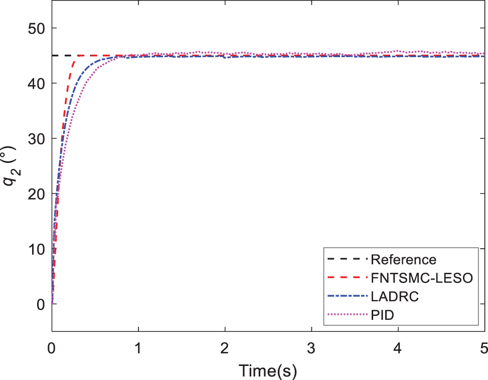
Figure 8: Response of joint 2 in Case B

Figure 9: Tracking errors of joint 1 in Case B

Figure 10: Tracking errors of joint 2 in Case B

Figure 11: Comparison of torque 1 in Case B

Figure 12: Comparison of torque 2 in Case B

Case C. In this simulation, the motion of the quadrotor and aerial manipulator are simulated. A special reference trajectory is set for the quadrotor which describes the phase from take-off to hover, as shown in Fig. 13. The controller parameters of PID are listed in Table 3. It can be observed that the quadrotor can track the reference trajectory well with the PID controller. Furthermore, the responses of the attitude and position are given in Figs. 14 and 15. When the quadrotor is in the hovering state, the reference trajectory of the manipulator is designed through the Cycloidal curve [52], and the initial angle of the two joints is set to 0. Considering that the manipulator will face the influence of disturbances, such as gust of wind, flexible deformation of the rope and mechanical vibration during actual work, a Gaussian noise with an amplitude of 1 N is added as the disturbance torque. The entire simulation time is set to 35 s. Similarly, LADRC and PID are used to control the cable-driven aerial manipulator respectively in the same environment, so as to compare the practicability of the three controllers. Figs. 16 and 17 show the output responses of the two joint angles under the three controllers. It can be seen that the three controllers can make the joint angles better track the reference trajectory. Furthermore, Figs. 18 and 19 show the tracking errors based on different controllers, and it can be seen that the trajectory tracking error obtained by the controller in this paper is the smallest. The root mean square error RMSE is used to evaluate the tracking accuracy. For q1, the RMSE of the controller in this paper is 0.638 which is 0.341 and 0.452 lower than that of LADRC and PID, respectively. For q2, the RMSE of the controller in this paper is 0.832, which is 0.299 and 0.557 lower than the RMSE of the latter two, respectively. This shows that the controller in this paper has high tracking accuracy and can effectively suppress the aggregate disturbance of the system. Finally, Figs. 20 and 21 show the comparison of the control torque of the three controllers. It can be observed from the figures that the proposed controller is the smoothest with almost no chattering phenomenon, which causes no harm to the actuator.

Figure 13: 3D flight trajectory of the quadrotor

Figure 14: Attitude response of the quadrotor

Figure 15: Position response of the quadrotor

Figure 16: Response of joint 1 in Case C

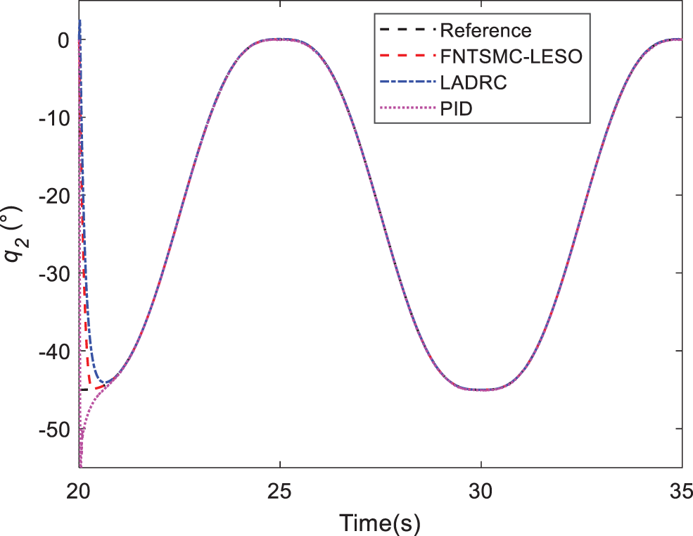
Figure 17: Response of joint 2 in Case C

Figure 18: Tracking errors of joint 1 in Case C

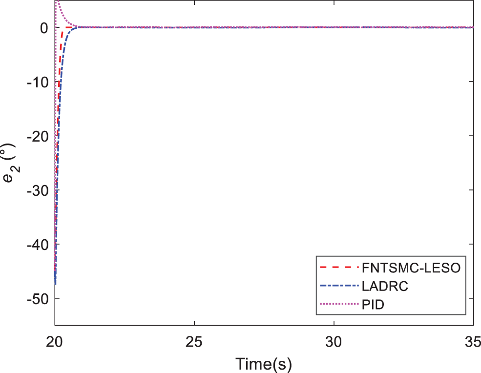
Figure 19: Tracking errors of joint 2 in Case C

Figure 20: Comparison of torque 1 in Case C

Figure 21: Comparison of torque 2 in Case C

6  Conclusions

In this paper, we have designed a novel cable-driven aerial manipulator applied for aerial tasks. Due to the use of cable-driven technology, the drive unit of the manipulator can be mounted at the base of the arm, simplifying the structure of the arm and reducing its quality. Meanwhile, a FNTSMC-LESO controller was proposed by combing the FNTMSC method with LESO technique. By using a nonlinear sliding mode surface, the FNTSMC-LESO control is capable of generating high precision and fast convergence. The nonlinear sliding mode surface, FNTSMC, can accelerate convergence in the region of the equilibrium point, which is of benefit to comprehensive performance. Furthermore, the parameter tuning of the proposed controller is conducted by ISSA. The simulation cases indicate that the proposed controller achieves a better control effect compared to LADRC and PID controllers.

In the future research, we will explore the other control strategy of the aerial manipulator and test the effectiveness of the proposed controller designed in this paper in the outdoor real flight test. In addition, we will further study the dynamic coupling law between the quadrotor and the cable-driven manipulator.

Acknowledgement: We would like to express our gratitude to the anonymous reviewers for their informative and constructive comments.

Funding Statement: This work was partially supported by the National Natural Science Foundation of China (52005231), Social Development Science and Technology Support Project of Changzhou (CE20215050), Jiangsu Province Graduate Student Practice Innovation Plan (SJCX21_1313, SJCX21_1314).

Conflicts of Interest: The authors declare that they have no conflicts of interest to report regarding the present study.

References

1. Guo, P., Xu, K., Deng, H., Liu, H., Ding, X. (2021). Modeling and control of a hexacopter with a passive manipulator for aerial manipulation. Complex & Intelligent Systems, 7(6), 3051–3065. DOI 10.1007/s40747-021-00488-6. [Google Scholar] [CrossRef]
2. Ding, X. L., Guo, P., Xu, K., Yu, Y. S. (2019). A review of aerial manipulation of small-scale rotorcraft unmanned robotic systems. Chinese Journal of Aeronautics, 32(1), 200–214. DOI 10.1016/j.cja.2018.05.012. [Google Scholar] [CrossRef]
3. Baizid, K., Giglio, G., Pierri, F., Trujillo, M. A., Antonelli, G. et al. (2017). Behavioral control of unmanned aerial vehicle manipulator systems. Autonomous Robots, 41(5), 1203–1220. DOI 10.1007/s10514-016-9590-0. [Google Scholar] [CrossRef]
4. Ramon-Soria, P., Arrue, B. C., Ollero, A. (2020). Grasp planning and visual servoing for an outdoors aerial dual manipulator. Engineering, 6(1), 77–88. DOI 10.1016/j.eng.2019.11.003. [Google Scholar] [CrossRef]
5. Ikeda, T., Minamiyama, S., Yasui, S., Ohara, K., Ichikawa, A. et al. (2019). Stable camera position control of unmanned aerial vehicle with three-degree-of-freedom manipulator for visual test of bridge inspection. Journal of Field Robotics, 36(7), 1212–1221. DOI 10.1002/rob.21899. [Google Scholar] [CrossRef]
6. Kim, S., Seo, H., Shin, J., Kim, H. J. (2018). Cooperative aerial manipulation using multirotors with multi-dof robotic arms. IEEE/ASME Transactions on Mechatronics, 23(2), 702–713. DOI 10.1109/TMECH.3516. [Google Scholar] [CrossRef]
7. Wang, Y., Li, B., Yan, F., Chen, B. (2019). Practical adaptive fractional-order nonsingular terminal sliding mode control for a cable-driven manipulator. International Journal of Robust and Nonlinear Control, 29(5), 1396–1417. DOI 10.1002/rnc.4441. [Google Scholar] [CrossRef]
8. Wang, Y., Yan, F., Chen, J., Ju, F., Chen, B. (2018). A new adaptive time-delay control scheme for cable-driven manipulators. IEEE Transactions on Industrial Informatics, 15(6), 3469–3481. DOI 10.1109/TII.9424. [Google Scholar] [CrossRef]
9. Beikzadeh, H., Liu, G., (2018). Trajectory tracking of quadrotor flying manipulators using L1 adaptive control. Journal of the Franklin Institute, 355(14), 6239–6261. DOI 10.1016/j.jfranklin.2018.06.011. [Google Scholar] [CrossRef]
10. Ma, L., Yan, Y., Li, Z., Liu, J. (2021). A novel aerial manipulator system compensation control based on ADRC and backstepping. Scientific Reports, 11(1), 1–15. DOI 10.1038/s41598-021-01628-1. [Google Scholar] [CrossRef]
11. Aydemir, M., Arıkan, K. B. (2020). Evaluation of the disturbance rejection performance of an aerial manipulator. Journal of Intelligent & Robotic Systems, 97(3), 451–469. DOI 10.1007/s10846-019-01013-1. [Google Scholar] [CrossRef]
12. Orsag, M., Korpela, C., Bogdan, S., Oh, P. (2017). Dexterous aerial robots—mobile manipulation using unmanned aerial systems. IEEE Transactions on Robotics, 33(6), 1453–1466. DOI 10.1109/TRO.2017.2750693. [Google Scholar] [CrossRef]
13. Kim, S., Seo, H., Choi, S., Kim, H. J. (2016). Vision-guided aerial manipulation using a multirotor with a robotic arm. IEEE/ASME Transactions on Mechatronics, 21(4), 1912–1923. DOI 10.1109/TMECH.2016.2523602. [Google Scholar] [CrossRef]
14. Yang, L., Yang, J. (2011). Nonsingular fast terminal sliding-mode control for nonlinear dynamical systems. International Journal of Robust and Nonlinear Control, 21(16), 1865–1879. DOI 10.1002/rnc.1666. [Google Scholar] [CrossRef]
15. Madani, T., Daachi, B., Djouani, K. (2016). Non-singular terminal sliding mode controller: Application to an actuated exoskeleton. Mechatronics, 33, 136–145. DOI 10.1016/j.mechatronics.2015.10.012. [Google Scholar] [CrossRef]
16. Yi, S., Zhai, J. (2019). Adaptive second-order fast nonsingular terminal sliding mode control for robotic manipulators. ISA Transactions, 90, 41–51. DOI 10.1016/j.isatra.2018.12.046. [Google Scholar] [CrossRef]
17. Li, S., Zhou, M., Yu, X. (2012). Design and implementation of terminal sliding mode control method for PMSM speed regulation system. IEEE Transactions on Industrial Informatics, 9(4), 1879–1891. DOI 10.1109/TII.2012.2226896. [Google Scholar] [CrossRef]
18. Miao, Y., Hwang, I., Liu, M., Wang, F. (2019). Adaptive fast nonsingular terminal sliding mode control for attitude tracking of flexible spacecraft with rotating appendage. Aerospace Science and Technology, 93, 105312. DOI 10.1016/j.ast.2019.105312. [Google Scholar] [CrossRef]
19. Ríos, H., Falcón, R., González, O. A., Dzul, A. (2018). Continuous sliding-mode control strategies for quadrotor robust tracking: Real-time application. IEEE Transactions on Industrial Electronics, 66(2), 1264–1272. DOI 10.1109/TIE.41. [Google Scholar] [CrossRef]
20. Chen, W. H., Ballance, D. J., Gawthrop, P. J., Gribble, J. J., O’Reilly, J. (1999). A nonlinear disturbance observer for two link robotic manipulators. Proceedings of the 38th IEEE Conference on Decision and Control, pp. 3410–3415. Phoenix, USA. [Google Scholar]
21. Chang, Z. Y., Luo, Y. Y., Shao, Y. H., Chu, H. Y., Wu, B. et al. (2020). Fuzzy sliding mode control for rotorcraft aerial manipulator with extended state observer. 2020 Chinese Automation Congress (CAC), pp. 1710–1714. IEEE, Shanghai, China. [Google Scholar]
22. Liu, J., Vazquez, S., Wu, L., Marquez, A., Gao, H. et al. (2016). Extended state observer-based sliding-mode control for three-phase power converters. IEEE Transactions on Industrial Electronics, 64(1), 22–31. DOI 10.1109/TIE.2016.2610400. [Google Scholar] [CrossRef]
23. Zhang, B., Tan, W., Li, J. (2019). Tuning of linear active disturbance rejection controller with robustness specification. ISA Transactions, 85, 237–246. DOI 10.1016/j.isatra.2018.10.018. [Google Scholar] [CrossRef]
24. Hekimoğlu, B. (2019). Optimal tuning of fractional order PID controller for DC motor speed control via chaotic atom search optimization algorithm. IEEE Access, 7, 38100–38114. DOI 10.1109/Access.6287639. [Google Scholar] [CrossRef]
25. Isiet, M., Gadala, M. (2020). Sensitivity analysis of control parameters in particle swarm optimization. Journal of Computational Science, 41, 101086. DOI 10.1016/j.jocs.2020.101086. [Google Scholar] [CrossRef]
26. Yan, F., Wang, Y., Xu, W., Chen, B. (2018). Time delay control of cable-driven manipulators with artificial bee colony algorithm. Transactions of the Canadian Society for Mechanical Engineering, 42(2), 177–186. DOI 10.1139/tcsme-2017-0043. [Google Scholar] [CrossRef]
27. Salloom, T., Yu, X., He, W., Kaynak, O. (2020). Adaptive neural network control of underwater robotic manipulators tuned by a genetic algorithm. Journal of Intelligent & Robotic Systems, 97(3), 657–672. DOI 10.1007/s10846-019-01008-y. [Google Scholar] [CrossRef]
28. Kommula, B. N., Kota, V. R. (2020). Direct instantaneous torque control of brushless DC motor using firefly algorithm based fractional order PID controller. Journal of King Saud University-Engineering Sciences, 32(2), 133–140. DOI 10.1016/j.jksues.2018.04.007. [Google Scholar] [CrossRef]
29. Singh, A., Sharma, V. (2019). Salp swarm algorithm-based model predictive controller for frequency regulation of solar integrated power system. Neural Computing and Applications, 31(12), 8859–8870. DOI 10.1007/s00521-019-04422-3. [Google Scholar] [CrossRef]
30. Mirjalili, S., Gandomi, A. H., Mirjalili, S. Z., Saremi, S., Faris, H. et al. (2017). Salp swarm algorithm: A bio-inspired optimizer for engineering design problems. Advances in Engineering Software, 114, 163–191. DOI 10.1016/j.advengsoft.2017.07.002. [Google Scholar] [CrossRef]
31. Fanni, M., Khalifa, A. (2017). A new 6-DOF quadrotor manipulation system: Design, kinematics, dynamics and control. IEEE/ASME Transactions on Mechatronics, 22(3), 1315–1326. DOI 10.1109/TMECH.2017.2681179. [Google Scholar] [CrossRef]
32. Jimenez-Cano, A., Braga, J., Heredia, G., Ollero, A. (2015). Aerial manipulator for structure inspection by contact from the underside. 2015 IEEE/RSJ International Conference on Intelligent Robots and Systems (IROS), pp. 1879–1884. IEEE, Hamburg, Germany. [Google Scholar]
33. Jimenez-Cano, A., Heredia, G., Bejar, M., Kondak, K., Ollero, A. (2016). Modelling and control of an aerial manipulator consisting of an autonomous helicopter equipped with a multi-link robotic arm. Proceedings of the Institution of Mechanical Engineers, Part G: Journal of Aerospace Engineering, 230(10), 1860–1870. [Google Scholar]
34. Kim, S. J., Lee, D. Y., Jung, G. P., Cho, K. J. (2018). An origami-inspired, self-locking robotic arm that can be folded flat. Science Robotics, 3(16eaar2915. DOI 10.1126/scirobotics.aar2915. [Google Scholar] [CrossRef]
35. Zhong, H., Miao, Z., Wang, Y., Mao, J., Li, L. et al. (2019). A practical visual servo control for aerial manipulation using a spherical projection model. IEEE Transactions on Industrial Electronics, 67(12), 10564–10574. DOI 10.1109/TIE.41. [Google Scholar] [CrossRef]
36. Chang, H., Liu, Y., Wang, Y., Zheng, X. (2017). A modified nonlinear dynamic inversion method for attitude control of UAVs under persistent disturbances. 2017 IEEE International Conference on Information and Automation (ICIA), pp. 715–721. IEEE, Macao. [Google Scholar]
37. Shi, D. J., Dai, X. H., Zhang, X. W., Quan, Q. (2017). A practical performance evaluation method for electric multicopters. IEEE-ASME Transactions on Mechatronics, 22(3), 1337–1348. DOI 10.1109/TMECH.2017.2675913. [Google Scholar] [CrossRef]
38. Tian, B. L., Lu, H. C., Zuo, Z. Y., Zong, Q., Zhang, Y. P. (2018). Multivariable finite-time output feedback trajectory tracking control of quadrotor helicopters. International Journal of Robust and Nonlinear Control, 28(1), 281–295. DOI 10.1002/rnc.3869. [Google Scholar] [CrossRef]
39. Wang, B., Zhang, Y. M. (2018). An adaptive fault-tolerant sliding mode control allocation scheme for multirotor helicopter subject to simultaneous actuator faults. IEEE Transactions on Industrial Electronics, 65(5), 4227–4236. DOI 10.1109/TIE.41. [Google Scholar] [CrossRef]
40. Dai, X., Ke, C., Quan, Q., Cai, K. Y. (2021). RFlySim: Automatic test platform for UAV autopilot systems with FPGA-based hardware-in-the-loop simulations. Aerospace Science and Technology, 114, 1–14. DOI 10.1016/j.ast.2021.106727. [Google Scholar] [CrossRef]
41. Dhadekar, D. D., Sanghani, P. D., Mangrulkar, K., Talole, S. (2021). Robust control of quadrotor using uncertainty and disturbance estimation. Journal of Intelligent & Robotic Systems, 101(3), 1–21. DOI 10.1007/s10846-021-01325-1. [Google Scholar] [CrossRef]
42. Tang, P., Zhang, F., Ye, J., Lin, D. (2021). An integral TSMC-based adaptive fault-tolerant control for quadrotor with external disturbances and parametric uncertainties. Aerospace Science and Technology, 109, 1–13. DOI 10.1016/j.ast.2020.106415. [Google Scholar] [CrossRef]
43. Azar, A. T., Serrano, F. E., Koubâa, A., Kamal, N. A., Vaidyanathan, S. et al. (2019). Adaptive terminal-integral sliding mode force control of elastic joint robot manipulators in the presence of hysteresis. International Conference on Advanced Intelligent Systems and Informatics, pp. 266–276. Springer, Tokyo, Japan. [Google Scholar]
44. Giusti, A., Malzahn, J., Tsagarakis, N. G., Althoff, M. (2018). On the combined inverse-dynamics/passivity-based control of elastic-joint robots. IEEE Transactions on Robotics, 34(6), 1461–1471. DOI 10.1109/TRO.8860. [Google Scholar] [CrossRef]
45. Wang, Y., Zhang, R., Ju, F., Zhao, J., Chen, B. et al. (2020). A light cable-driven manipulator developed for aerial robots: Structure design and control research. International Journal of Advanced Robotic Systems, 17(3), 1–14. DOI 10.1177/1729881420926425. [Google Scholar] [CrossRef]
46. Zhao, J., Wang, Y., Wang, D., Ju, F., Chen, B. et al. (2020). Practical continuous nonsingular terminal sliding mode control of a cable-driven manipulator developed for aerial robots. Proceedings of the Institution of Mechanical Engineers, Part I: Journal of Systems and Control Engineering, 234(9), 1011–1023. DOI 10.1177/0959651819899494. [Google Scholar] [CrossRef]
47. Yu, S., Yu, X., Shirinzadeh, B., Man, Z. (2005). Continuous finite-time control for robotic manipulators with terminal sliding mode. Automatica, 41(11), 1957–1964. DOI 10.1016/j.automatica.2005.07.001. [Google Scholar] [CrossRef]
48. Salgotra, R., Singh, U., Singh, S., Singh, G., Mittal, N. (2021). Self-adaptive salp swarm algorithm for engineering optimization problems. Applied Mathematical Modelling, 89, 188–207. DOI 10.1016/j.apm.2020.08.014. [Google Scholar] [CrossRef]
49. Li, S., Wang, G., Yang, J. (2019). Survey on cloud model based similarity measure of uncertain concepts. CAAI Transactions on Intelligence Technology, 4(4), 223–230. DOI 10.1049/trit.2019.0021. [Google Scholar] [CrossRef]
50. Wang, P., Xu, X., Huang, S., Cai, C. (2018). A linguistic large group decision making method based on the cloud model. IEEE Transactions on Fuzzy Systems, 26(6), 3314–3326. DOI 10.1109/TFUZZ.2018.2822242. [Google Scholar] [CrossRef]
51. Zhao, D., Li, C., Wang, Q., Yuan, J. (2020). Comprehensive evaluation of national electric power development based on cloud model and entropy method and TOPSIS: A case study in 11 countries. Journal of Cleaner Production, 277, 1–14. DOI 10.1016/j.jclepro.2020.123190. [Google Scholar] [CrossRef]
52. Kali, Y., Saad, M., Benjelloun, K., Khairallah, C. (2018). Super-twisting algorithm with time delay estimation for uncertain robot manipulators. Nonlinear Dynamics, 93(2), 557–569. DOI 10.1007/s11071-018-4209-y. [Google Scholar] [CrossRef]
Cite This Article
Copyright © 2023 The Author(s). Published by Tech Science Press.
This work is licensed under a Creative Commons Attribution 4.0 International License , which permits unrestricted use, distribution, and reproduction in any medium, provided the original work is properly cited.
Downloads
Citation Tools