
 Submit a Paper
 Propose a Special lssue
 Open Access
ARTICLE
Bayesian Computation for the Parameters of a Zero-Inflated Cosine Geometric Distribution with Application to COVID-19 Pandemic Data
Department of Applied Statistics, Faculty of Applied Science, King Mongkut’s University of Technology North Bangkok, Bangkok, 10800, Thailand
* Corresponding Author: Sa-Aat Niwitpong. Email:
(This article belongs to the Special Issue: New Trends in Statistical Computing and Data Science)
Computer Modeling in Engineering & Sciences 2023, 135(2), 1229-1254. https://doi.org/10.32604/cmes.2022.022098
Received 21 February 2022; Accepted 08 June 2022; Issue published 27 October 2022
 View Full Text
 Download PDF
Abstract
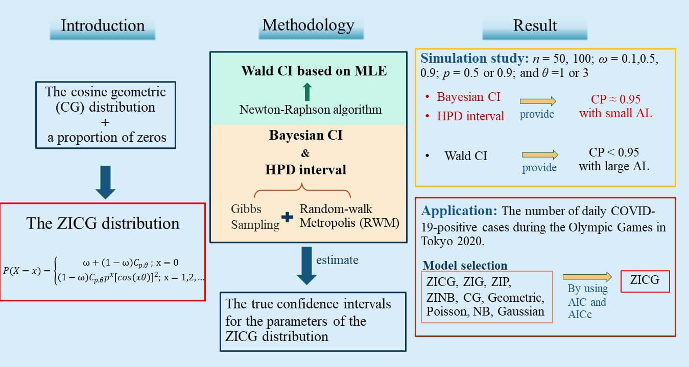
A new three-parameter discrete distribution called the zero-inflated cosine geometric (ZICG) distribution is proposed for the first time herein. It can be used to analyze over-dispersed count data with excess zeros. The basic statistical properties of the new distribution, such as the moment generating function, mean, and variance are presented. Furthermore, confidence intervals are constructed by using the Wald, Bayesian, and highest posterior density (HPD) methods to estimate the true confidence intervals for the parameters of the ZICG distribution. Their efficacies were investigated by using both simulation and real-world data comprising the number of daily COVID-19 positive cases at the Olympic Games in Tokyo 2020. The results show that the HPD interval performed better than the other methods in terms of coverage probability and average length in most cases studied.Graphic Abstract
Keywords
Over-dispersed count data with excess zeros occur in various situations, such as the number of torrential rainfall incidences at the Daegu and the Busan rain gauge stations in South Korea [1], the DMFT (decayed, missing, and filled teeth) index in dentistry [2], and the number of falls in a study on Parkinson’s disease [3]. Classical models such as Poisson, geometric, and negative binomial (NB) distributions may not be suitable for analyzing these data, so two classes of modified count models (zero-inflated (ZI) and hurdle) are used instead. Both can be viewed as finite mixture models comprising two components: for the zero part, a degenerate probability mass function is used in both, while for the non-zero part, a zero-truncated probability mass function is used in hurdle models and an untruncated probability mass function is used in ZI models. Poisson and geometric hurdle models were proposed and used by [4] to analyze data on the daily consumption of various beverages; in the intercept-only case (no regressors appear in either part of the model), the ZI model is equivalent to the hurdle model, with the estimation yielding the same log-likelihood and fitted probabilities. Furthermore, several comparisons with classical models have been reported in the literature. The efficacies of ZI and hurdle models have been explored by comparing least-squares regression with transformed outcomes (LST), Poisson regression, NB regression, ZI Poisson (ZIP), ZINB, zero-altered Poisson (ZAP) (or Poisson hurdle), and zero-altered NB (ZANB) (or NB hurdle) models [5]; the results from using both simulated and real data on health surveys show that the ZANB and ZINB models performed better than the others when the data had excess zeros and were over-dispersed. Recently, Feng [6] reviewed ZI and hurdle models and highlighted their differences in terms of their data-generating process; they conducted simulation studies to evaluate the performances of both types of models, which were found to be dependent on the percentage of zero-deflated data points in the data and discrepancies between structural and sampling zeros in the data-generating process.
The main idea of a ZI model is to add a proportion of zeros to the baseline distribution [7,8], for which various classical count models (e.g., ZIP, ZINB, and ZI geometric (ZIG)), are available. These have been studied in several fields and many statistical tools have been used to analyze them. The ZIP distribution originally proposed by [9] has been studied by various researchers. For instance, Ridout et al. [10] considered the number of roots produced by 270 shoots of Trajan apple cultivars (the number of shoots entries provided excess zeros in the data), and analyzed the data by using Poisson, NB, ZIP, and ZINB models; the fits of these models were compared by using the Akaike information criterion (AIC) and the Bayesian information criterion (BIC), the results of which show that ZINB performed well. Yusuf et al. [11] applied the ZIP and ZINB regression models to data on the number of falls by elderly individuals; the results show that the ZINB model attained the best fit and was the best model for predicting the number of falls due to the presence of excess zeros and over-dispersion in the data. Iwunor [12] studied the number of male rural migrants from households by using an inflated geometric distribution and estimated the parameters of the latter; the results show that the maximum likelihood estimates were not too different from the method of moments values. Kusuma et al. [13] showed that a ZIP regression model is more suitable than an ordinary Poisson regression model for modeling the frequency of health insurance claims.
The cosine geometric (CG) distribution, a newly reported two-parameter discrete distribution belonging to the family of weighted geometric distributions [14], is useful for analyzing over-dispersed data and has outperformed some well-known models such as Poisson, geometric, NB, and weighted NB. In the present study, the CG distribution was applied as the baseline and then a proportion of zeros was added to it, resulting in a novel three-parameter discrete distribution called the ZICG distribution.
Statistical tools such as confidence intervals provide more information than point estimation and p-values for statistical inference [15]. Hence, they have often been applied to analyze ZI count data. For example, Wald confidence intervals for the parameters in the Bernoulli component of ZIP and ZAP models were constructed by [16], while Waguespack et al. [17] provided a Wald-based confidence interval for the ZIP mean. Moreover, Srisuradetchai et al. [18] proposed the profile-likelihood-based confidence interval for the geometric parameter of a ZIG distribution. Junnumtuam et al. [19] constructed Wald confidence intervals for the parameters of a ZIP model; in an analysis of the number of daily COVID-19 deaths in Thailand using six models: Poisson, NB, geometric, Gaussian, ZIP, and ZINB, they found that the Wald confidence intervals for the ZIP model were the most suitable. Furthermore, Srisuradetchai et al. [20] proposed three confidence intervals: a Wald confidence interval and score confidence intervals using the profile and the expected or observed Fisher information for the Poisson parameter in a ZIP distribution; the latter two outperformed the Wald confidence interval in terms of coverage probability, average length, and the coverage per unit length.
Besides the principal method involving maximum likelihood estimation widely used to estimate parameters in ZI count models, Bayesian analysis is also popular. For example, Cancho et al. [21] provided a Bayesian analysis for the ZI hyper-Poisson model by using the Markov chain Monte Carlo (MCMC) method; they used some noninformative priors in the Bayesian procedure and compared the Bayesian estimators with maximum likelihood estimates obtained by using the Newton-Raphson method and found that all of the estimates were close to the real values of the parameters as the sample size was increased, which means that their biases and mean-squared errors (MSEs) approached zero under this circumstance. Recently, Workie et al. [22] applied the Bayesian analytic approach by using MCMC simulation and Gibbs’ sampling algorithm for modeling the Bayesian ZI regression model determinants to analyze under-five child mortality.
Motivated by these previous studies, we herein propose Wald confidence intervals based on maximum likelihood estimation, Bayesian credible intervals, and highest posterior density (HPD) intervals for the three parameters of a ZICG distribution. Both simulated data and real-world data were used to compare the efficacies of the proposed methods for constructing confidence intervals via their coverage probabilities and average lengths.
The CG distribution is a two-parameter discrete distribution belonging to the family of weighted geometric distributions [14]. The probability mass function (PMF) for a CG distribution is given by
where
If
where
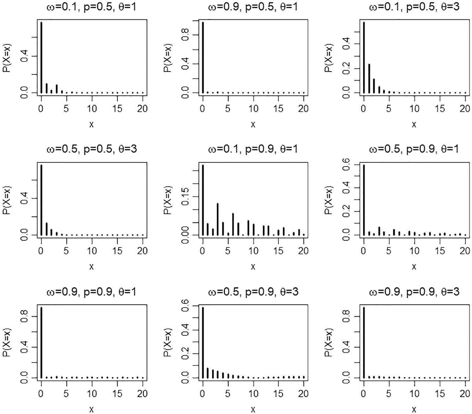
Figure 1: Pmf plots of the ZICG distribution for different values of the parameters
This section provides the cumulative distribution function (CDF), moment generating function (MGF), mean, and variance of a ZICG distribution, which are derived from the CG distribution [14].
Proposition 2.1. The cdf of a ZICG distribution with parameters
Proposition 2.2. The mgf of the ZICG distribution with parameters
Since the explicit expression for the moment using equality is
Since
and
Since
The index of dispersion (D), a measure of dispersion, is defined as the ratio of the variance to the mean
The values of D for selected values of the parameters

2.3 Maximum Likelihood Estimation for the ZICG Model with No Covariates
The likelihood function of the ZICG distribution is
while the log-likelihood function of the ZICG distribution can be expressed as
In the case of a single homogeneous sample (p,
where J is the largest observed count value;
Here, we have

This provides the closed-form expression for
2.4 The Wald Confidence Intervals for the ZICG Parameters
In this study, we assume that there is more than one unknown parameter. Meanwhile, the assumed parameter vector is
where standard error
where
where
where
Hence, the
where

2.5 Bayesian Analysis for the Confidence Intervals for the ZICG Parameters
Suppose
Let
Since the elements in set A can be generated from two different parts: (1) the real zeros part and (2) the CG distribution, after which the an unobserved latent allocation variable can be defined as
where
Thus, the likelihood function based on augmented data
where
and
Since there is no prior information from historic data or previous experiments, we use the noninformative prior for all of the parameters. The prior distributions for
where
the joint posterior distribution for parameters
Since the joint posterior distribution in (35) is analytically intractable for calculating the Bayes estimates similarly to using the posterior distribution method, MCMC simulation can be applied to generate the parameters [26,27]. The Metropolis-Hastings algorithm is an MCMC method for obtaining a sequence of random samples from a probability distribution from which direct sampling is difficult. Subsequently, the obtained sequence can be used to approximate the desired distribution. Moreover, the Gibbs’ sampler, which is an alternative to the Metropolis-Hastings algorithm for sampling from the posterior distribution of the model parameters, can be used. Hence, the Gibbs’ sampler can be applied to generate samples from the joint posterior distribution in (35). Clearly, the marginal posterior distribution of
Thus, the marginal posterior distribution of
and the marginal posterior distribution of
Here, we applied the random-walk Metropolis (RWM) algorithm to generate p and
The process proceeds as follows:
1. Choose trial position
2. Calculate
3. Generate
4. If
The Gibbs’ sampling steps are as follows:

2.6 The Bayesian-Based HPD Interval
The HPD interval is the shortest Bayesian credible interval containing
1. The density for each point inside the interval is greater than that for each point outside of it.
2. For a given probability (say 1 −
Bayesian credible intervals can be obtained by using the MCMC method [30]. Hence, we used it to construct HPD intervals for the parameters of a ZICG distribution. This approach only requires MCMC samples generated from the marginal posterior distributions of the three parameters:

2.7 The Efficacy Comparison Criteria
Coverage probabilities and average lengths were used to compare the efficacies of the confidence intervals. Suppose the nominal confidence level is
and the average length is computed by
where
Sample size
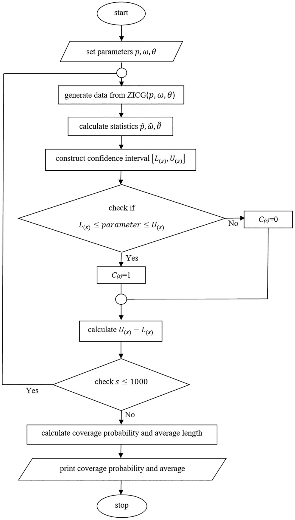
Figure 2: A flowchart of the simulation study

For sample size n = 50 or 100, the Bayesian credible intervals and the HPD intervals performed better than the Wald confidence intervals because they provided coverage probabilities close to the nominal confidence level (0.95) and obtained the shorter average lengths for almost all of the cases. However, when the proportion of zeros was high (i.e.,
3.2 Applicability of the Methods When Using Real COVID-19 Data
Data for new daily COVID-19 cases during the Tokyo 2020 Olympic Games from 01 July 2021 to 12 August 2021 were used for this demonstration. The data are reported by the Tokyo Organizing Committee on the Government website (https://olympics.com/en/olympic-games/tokyo-2020) and they are shown in Table 3, with a histogram of the data provided in Fig. 3.

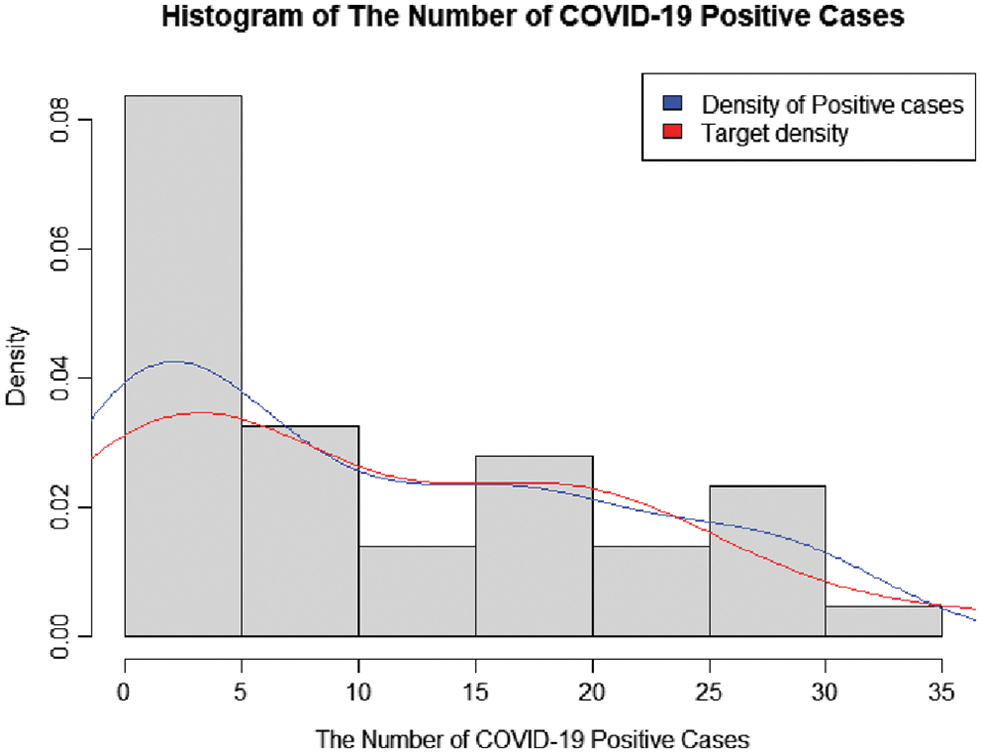
Figure 3: A histogram of the number of COVID-19-positive case during the olympic games in Tokyo 2020
3.2.1 Analysis of the COVID-19 Data
The information in Table 4 shows that the data are over-dispersed with an index of dispersion of 9.7149. The suitability of fitting the data to ZICG, ZIG, ZIP, ZINB, CG, geometric, Poisson, NB, and Gaussian distributions was assessed by using the AIC computed as AIC


The 95

We proposed a new mixture distribution called ZICG and presented its properties, namely the mgf, mean, variance, and Fisher information. According to the empirical study results, the ZICG distribution is suitable for over-dispersed count data containing excess zeros, such as occurred in the number of daily COVID-19-positive cases at the Tokyo 2020 Olympic Games. Confidence intervals for the three parameters of the ZICG distribution were constructed by using the Wald confidence interval, the Bayesian credible interval, and the HPD interval. Since the maximum likelihood estimates of the ZICG model parameters have no closed form, the Newton-Raphson method was applied to estimate the parameters and construct the Wald confidence intervals. Furthermore, Gibbs’ sampling with the RWM algorithm was utilized in the Bayesian computation to approximate the parameters and construct the Bayesian credible intervals and the HPD intervals. Their performances were compared in terms of coverage probabilities and average lengths. According to the simulation results, the index of dispersion plays an important role: when it was small (e.g.,
Acknowledgement: The first author acknowledges the generous financial support from the Science Achievement Scholarship of Thailand (SAST).
Funding Statement: This research has received funding support from the National Science, Research and Innovation Fund (NSRF), and King Mongkut’s University of Technology North Bangkok (Grant No. KMUTNB-FF-65-22).
Conflicts of Interest: The authors declare that they have no conflicts of interest to report regarding the present study.
References
1. Lee, C., Kim, S. (2017). Applicability of zero-inflated models to fit the torrential rainfall count data with extra zeros in South Korea. Water, 9(2), 123. DOI 10.3390/w9020123. [Google Scholar] [CrossRef]
2. Böhning, D., Dietz, E., Schlattmann, P., Mendonca, L., Kirchner, U. (1999). The zero-inflated poisson model and the decayed, missing and filled teeth index in dental epidemiology. Journal of the Royal Statistical Society: Series A (Statistics in Society), 162(2), 195–209. DOI 10.1111/1467-985X.00130. [Google Scholar] [CrossRef]
3. Ashburn, A., Fazakarley, L., Ballinger, C., Pickering, R., McLellan, L. D. et al. (2006). A randomised controlled trial of a home based exercise programme to reduce the risk of falling among people with Parkinson’s disease. Journal of Neurology, Neurosurgery & Psychiatry, 78(7), 678–684. DOI 10.1136/jnnp.2006.099333. [Google Scholar] [CrossRef]
4. Mullahy, J. (1986). Specification and testing of some modified count data models. Journal of Econometrics, 33(3), 341–365. DOI 10.1016/0304-4076(86)90002-3. [Google Scholar] [CrossRef]
5. Yang, S., Harlow, L. L., Puggioni, G., Redding, C. A. (2017). A comparison of different methods of zero-inflated data analysis and an application in health surveys. Journal of Modern Applied Statistical Methods, 16(1), 518–543. DOI 10.22237/jmasm/1493598600. [Google Scholar] [CrossRef]
6. Feng, C. X. (2021). A comparison of zero-inflated and hurdle models for modeling zero-inflated count data. Journal of Statistical Distributions and Applications, 8(8), 1–19. [Google Scholar]
7. Cameron, A. C., Trivedi, P. K. (2013). Regression analysis of count data. New York, USA: Cambridge University Press. [Google Scholar]
8. Böhning, D., Ogden, H. (2021). General flation models for count data. Metrika, 84, 245–261. DOI 10.1007/s00184-020-00786-y. [Google Scholar] [CrossRef]
9. Lambert, D. (1992). Zero-inflated poisson regression, with an application to defects in manufacturing. Technometrics, 34(1), 1–14. DOI 10.2307/1269547. [Google Scholar] [CrossRef]
10. Ridout, M. S., Demetrio, C. G. B., Hinde, J. P. (1998). Models for counts data with many zeros. The 19th International Biometric Conference, Cape Town, South Africa. [Google Scholar]
11. Yusuf, O. B., Bello, T., Gureje, O. (2017). Zero inflated poisson and zero inflated negative binomial models with application to number of falls in the elderly. Biostatistics and Biometrics Open Access Journal, 1(4), 69–75. [Google Scholar]
12. Iwunor, C. C. (1995). Estimation of parameters of the inflated geometric distribution for rural out-migration. Genus, 51, 253–260. [Google Scholar]
13. Kusuma, R. D., Purwono, Y. (2019). Zero-inflated poisson regression analysis on frequency of health insurance claim pt. xyz. 12th International Conference on Business and Management Research, Bali, Indonesia. [Google Scholar]
14. Chesneau, C., Bakouch, H., Hussain, T., Para, B. (2021). The cosine geometric distribution with count data modeling. Journal of Applied Statistics, 48(1), 124–137. DOI 10.1080/02664763.2019.1711364. [Google Scholar] [CrossRef]
15. Das, S. K. (2019). Confidence interval is more informative than p-value in research. International Journal of Engineering Applied Sciences and Technology, 4(6), 278–282. DOI 10.33564/IJEAST.2019.v04i06.045. [Google Scholar] [CrossRef]
16. Srisuradetchai, P., Junnumtuam, S. (2020). Wald confidence intervals for the parameter in a Bernoulli component of zero-inflated poisson and zero-altered poisson models with different link functions. Science & Technology Asia, 25(2), 1–14. [Google Scholar]
17. Waguespack, D., Krishnamoorthy, K., Lee, M. (2020). Tests and confidence intervals for the mean of a zero-inflated poisson distribution. American Journal of Mathematical and Management Sciences, 39(4), 383–390. DOI 10.1080/01966324.2020.1777914. [Google Scholar] [CrossRef]
18. Srisuradetchai, P., Dangsupa, K. (2021). Profile-likelihood-based confidence intervals for the geometric parameter of the zero-inflated geometric distribution. The Journal of KMUTNB, 31(3), 527–538. DOI 10.14416/j.kmutnb. [Google Scholar] [CrossRef]
19. Junnumtuam, S., Niwitpong, S. A., Niwitpong, S. (2021). The Bayesian confidence interval for coefficient of variation of zero-inflated poisson distribution with application to daily COVID-19 deaths in Thailand. Emerging Science Journal, 5, 62–76. DOI 10.28991/esj-2021-SPER-05. [Google Scholar] [CrossRef]
20. Srisuradetchai, P., Tonprasongrat, K. (2022). On interval estimation of the poisson parameter in a zero-inflated poisson distribution. Thailand Statistician, 20(2), 357–371. [Google Scholar]
21. Cancho, V. G., Yiqi, B., Fiorucci, J. A., Barriga, G. D. C., Dey, D. K. (2017). Estimation and influence diagnostics for zero-inflated hyper-poisson regression model: Full Bayesian analysis. Communications in Statistics–Theory and Methods, 47(11), 2741–2759. DOI 10.1080/03610926.2017.1342839. [Google Scholar] [CrossRef]
22. Workie, M. S., Azene, A. G. (2021). Bayesian zero-inflated regression model with application to under-five child mortality. Journal of Big Data, 8(4), 1–23. [Google Scholar]
23. Bilder, C. R., Loughin, T. M. (2014). Analysis of categorical data with R. Boca Raton, FL, USA: CRC Press. [Google Scholar]
24. Team, R. C. (2021). R: A language and environment for statistical computing. R Foundation for Statistical Computing, Vienna, Austria. https://www.R-project.org/. [Google Scholar]
25. Tanner, M. A., Wong, W. H. (1987). The calculation of posterior distributions by data augmentation. Journal of the American Statistical Association, 82(398), 528–540. DOI 10.1080/01621459.1987.10478458. [Google Scholar] [CrossRef]
26. Hastings, W. K. (1970). Monte carlo sampling methods using markov chains and their applications. Biometrika, 57(1), 97–109. DOI 10.1093/biomet/57.1.97. [Google Scholar] [CrossRef]
27. Metropolis, N., Ulam, S. (1949). The monte carlo method. Journal of the American Statistical Association, 44(247), 335–341. DOI 10.1080/01621459.1949.10483310. [Google Scholar] [CrossRef]
28. Maima, D. H. M. (2015). On the random walk metropolis algorithm (Master’s Thesis). Islamic University of Gaza, Gaza. [Google Scholar]
29. Box, G. E. P., Tiao, G. C. (1992). Bayesian inference in statistical analysis. New York, USA: Wiley. [Google Scholar]
30. Chen, M. H., Shao, Q. M. (1999). Monte carlo estimation of Bayesian credible and HPD intervals. Journal of Computational and Graphical Statistics, 8(1), 69–92. [Google Scholar]
31. Meredith, M., Kruschke, J. (2020). HDInterval: Highest (Posterior) density intervals. https://CRAN.R-project.org/package=HDInterval. R package version 0.2.2. [Google Scholar]
32. Casella, G., Berger, R. L. (2002). Statistical inference. USA: Thomson Learning, Duxbury. [Google Scholar]
33. Daidoji, K., Iwasaki, M. (2012). On interval estimation of the poisson parameter in a zero-truncated poisson distribution. Journal of the Japanese Society of Computational Statistics, 25(1), 1–12. DOI 10.5183/jjscs.1103002_193. [Google Scholar] [CrossRef]
Appendix A.R code for simulation study
rCGD<−function(n, p, theta){
X = rep(0, n)
for (j in 1:n) {
i = 0
#step 1: Generated Uniform(0, 1)
U = runif(1, 0, 1)
#step 2: Computed F(k * − 1) and F(k * )
cdf<−(2 * (1 − p) * (1 − 2 * p * cos(2 * theta) + p∧2))
/(2 + p * ((p − 3) * cos(2 * theta) + p − 1))
while(U >= cdf)
{i = i + 1;
cdf = cdf + f(i, p, theta) }
X[j] = i;
}
return(X)
}
C<−function(p, theta) {
(2 * (1 − p) * (1 − 2 * p * cos(2 * theta) + p∧2))/(2 + p * ((p − 3) * cos(2 * theta) + p − 1))}
#Calculating log likelihood of CG
loglikeCG<−function(x, y) {
p<−x[1]
theta<−x[2]
loglike<− n * log(2) + n * log(1 − p)+
n * log(1 − 2 * p * cos(2 * theta) + p∧2)−
n * log(2 + p * ((p − 3) * cos(2 * theta) + p − 1))+
log(p) * sum(y) + 2 * sum(log(cos(y * theta)))
# note use of sum
loglike<− −loglike
}
#Calculating the log-likelihood for ZICG
loglikeZICG<−function(x, y) {
w<−x[1]
p<−x[2]
theta<−x[3]
n0<−length(y[which(y == 0)])
ypos<−y[which(y != 0)] #y > 0
loglike<− n0 * log(w + (1 − w) * C(p, theta))
+ sum(log((1 − w) * C(p, theta) *
(p∧ypos) * cos(ypos * theta)∧2))
loglike<− −loglike
}
# Bayesian Confidence Interval
gibbs<−function(y = y, sample.size, n, p, theta, w){
nonzero_values = y[which(y != 0)]
m<−n−length(nonzero_values)
ypos = y[which(y != 0)]
prob.temp = numeric()
S.temp = numeric()
theta.temp = numeric(sample.size)
w.temp = numeric(sample.size)
p.temp = numeric(sample.size)
p.temp[1]<−0.5 #initial p value
theta.temp[1]<−0.5 #initial theta
w.temp[1]<−0.5 #initial w value
prob.temp[1]<−w.temp[1]/(w.temp[1] + (1−w.temp[1]) * (2 * (1 − p.temp[1])
* 1 − 2 * p.temp[1] * cos(2 * theta.temp[1]) + p.temp[1]∧2))/(2 + p.temp[1] * ((p.temp[1] − 3)
* cos(2 * theta.temp[1]) + p.temp[1] − 1)))
S.temp[1]<−rbinom(1, m, prob.temp[1])
w.temp[1]<−rbeta(1,S.temp[1] + 0.5, n−S.temp[1] + 0.5)
p.samp<−GenerateMCMC.p(y = y, N = 1000, n = n, m = m, w = w.temp[1], theta = theta.temp[1],
sigma = 1)
p.temp[1]<−mean(p.samp[501:1000])
theta.samp<−GenerateMCMCsample(ypos = ypos,N = 1000, n = n, m = m, w = w.temp[1], p = p.temp[1],
sigma = 1)
theta.temp[1]<−mean(theta.samp[501:1000])
for(i in 2:(sample.size)){
prob.temp[i]<−w.temp[i − 1]/(w.temp[i − 1] + (1−w.temp[i − 1]) * C(p.temp[i − 1],
theta.temp[i − 1]))
S.temp[i]<−rbinom(1, m, prob.temp[i])
w.temp[i]<−rbeta(1,S.temp[i] + 0.5
, n−S.temp[i] + 0.5)
p.samp<−GenerateMCMC.p(y = y, N = 1000, n = n, m = m, w = w.temp[i],
theta = theta.temp[i − 1], sigma = 1)
p.temp[i]<−mean(p.samp[501:1000])
theta.samp<−GenerateMCMCsample(ypos = ypos,N = 1000, n = n, m = m, w = w.temp[i],
p = p.temp[i], sigma = 1)
theta.temp[i]<−mean(theta.samp[501:1000])}
return(cbind(w.temp, p.temp, theta.temp))}
#random walk Metropolis for sample theta
GenerateMCMCsample<−function(ypos,N, n, m, w, p, sigma){
prior <− function(x) dgamma(x, shape = 2, rate = 1/3)
theta.samp <− numeric(length = N)
theta.samp[1] <− runif(n = 1, min = 0, max = 5)
for (j in 2:N) {
Yj<−theta.samp[j − 1] + rnorm(n = 1, mean = 0, sigma)
if(0< = Yj&&Yj< = pi/2){
alpha.cri <−((w + (1 − w) * C(p,Yj))∧m * ((1 − w) * (2 * (1 − p) * (1 − 2 * p * cos(2 * Yj) + p∧2))/
(2 + p * ((p − 3) * cos(2 * Yj) + p − 1)))∧(n − m) * prod((cos(ypos * Yj))∧2) * prior(Yj))/
((w + (1 − w) * C(p, theta.samp[j − 1]))∧m * ((1 − w) * (2 * (1 − p) *
(1 − 2 * p * cos(2 * theta.samp[j − 1]) + p∧2))/
(2 + p * ((p − 3) * cos(2 * theta.samp[j − 1]) + p − 1)))∧(n − m) *
prod((cos(ypos * theta.samp[j − 1]))∧2) * prior(theta.samp[j − 1]))
}else{alpha.cri<− 0}
U <− runif(1)
if(is.na(alpha.cri)){theta.samp[j]<− theta.samp[j − 1]} else {
if (U < min(alpha.cri, 1))
{theta.samp[j]<− Yj
}else theta.samp[j]<− theta.samp[j − 1]}
} return(theta.samp)}
##Random Walk Metropolis sampler for p
GenerateMCMC.p <− function(y,N, n, m, w, theta, sigma){
prior<−function(x)dbeta(x, shape1 = 2,
shape2 = 5)
p.samp <− numeric(length = N)
p.samp[1] <− runif(n = 1, min = 0, max = 1)
for (j in 2:N) {
Yj<−p.samp[j − 1] + rnorm(n = 1, mean = 0, sigma)
if(0< = Yj&&Yj< = 1){
alpha.cri <−((w + (1 − w) * C(Yj, theta))∧m * ((1 − w) * C(Yj, theta))∧(n − m) * Yj∧(sum(y)))
* prior(Yj)/((w + (1 − w) * C(p.samp[j − 1], theta))∧m *
((1 − w) * C(p.samp[j − 1], theta))∧(n − m) * p.samp[j − 1]∧(sum(y))) * prior(p.samp[j − 1])
}else{alpha.cri<− 0 }
U <− runif(1)
if(is.na(alpha.cri)){
p.samp[j]<− p.samp[j − 1]}
else {if (U < min(alpha.cri, 1)) {
p.samp[j]<− Yj
}else p.samp[j]<− p.samp[j − 1]} }
return(p.samp)
}
i = 0
while(i<M){
suscept<−rbinom(n, size = 1, prob = 1 − w)
count<−rCGD(n , p, theta)
y = suscept * count
if(max(y) == 0){
next
}i = i + 1
p_hat<−egeom(y, method = “mle”)
p0 = p_hat$parameters;theta0 = 0.5;
# store starting values
intvalues1 = c(p0, theta0)
resultCG<−nlm(loglikeCG, intvalues1 , y, hessian = TRUE, print.level = 1)
mleCG<−resultCG$estimate
mleCG.p <− c(mleCG[1])
mleCG.theta<−c(mleCG[2])
#formula for estimating w (omega)
n0<−length(y[which(y == 0)])
p1 = mleCG.p ; theta1 = mleCG.theta;
c_hat<−C(p1, theta1)
w1<−(n0 − n * c_hat)/(n * (1 − c_hat))
intvalues2 = c(w1, p1, theta1)
resultZICG<−nlm(loglikeZICG, intvalues2, y, hessian=TRUE, print.level = 1)
mleZICG<−resultZICG$estimate
hess<−resultZICG$hessian
cov<−solve(hess, tol = NULL)
stderr<−sqrt(diag(cov))
mle.w <− c(mleZICG[1])
mle.p <− c(mleZICG[2])
mle.theta<−c(mleZICG[3])
sd.w <− stderr[1]
sd.p <− stderr[2]
sd.theta <−stderr[3]
#Wald confidence interval for w
#lower bound of Wald CI for w
Wald.w.L[i]<−mle.w − qnorm(1 − alpha/2) * sd.w
#Upper bound of Wald CI for w
Wald.w.U[i]<−mle.w + qnorm(1 − alpha/2) * sd.w
Wald.CI.w = rbind(c(Wald.w.L[i],Wald.w.U[i]))
Wald.CP.w[i] = ifelse(Wald.w.L[i]<w&&w<Wald.w.U[i], 1, 0)
Wald.Length.w[i] = Wald.w.U[i] − Wald.w.L[i]
#Wald confidence interval for p
#lower bound of Wald CI for p
Wald.p.L[i]<−mle.p − qnorm(1 − alpha/2) * sd.p
#Upper bound of Wald CI for p
Wald.p.U[i]<−mle.p + qnorm(1 − alpha/2) * sd.p
Wald.CI.p = rbind(c(Wald.p.L[i],Wald.p.U[i]))
Wald.CP.p[i] = ifelse(Wald.p.L[i]<p&&<Wald.p.U[i], 1, 0)
Wald.Length.p[i] = Wald.p.U[i] − Wald.p.L[i]
#Wald confidence interval for theta
#lower bound of Wald CI for theta
Wald.theta.L[i]<−mle.theta − qnorm(1 − alpha/2) * sd.theta
#Upper bound of Wald CI for theta
Wald.theta.U[i]<−mle.theta + qnorm(1 − alpha/2) * sd.theta
Wald.CI.theta = rbind(c( Wald.theta.L[i],Wald.theta.U[i]))
Wald.CP.theta[i] = ifelse(Wald.theta.L[i]<theta&&theta<Wald.theta.U[i], 1, 0)
Wald.Length.theta[i] = Wald.theta.U[i] − Wald.theta.L[i]
#########End Wald CI#############
test<−gibbs(y = y, sample.size = sample.size,
n = n, p = p, theta = theta, w = w)
#burn-in w estimator
w.mcmc<−test[, 1][1001:3000]
#estimator of w
w.bayes<−mean(w.mcmc)
#burn-in p estimator
p.mcmc<−test[, 2][1001:3000]
#estimator of p
p.bayes<−mean(p.mcmc)
#burn-in theta estimator
theta.mcmc<−test[, 3][1001:3000]
#estimator of theta
theta.bayes<−mean(theta.mcmc)
#########Construct Bayesian confidence interval########
L.w[i] = quantile(w.mcmc, alpha/2, na.rm = TRUE)
U.w[i] = quantile(w.mcmc,(1 − alpha/2), na.rm = TRUE)
CIr1 = rbind(c(L.w[i],U.w[i]))
Bayes.CP.w[i] = ifelse(L.w[i]<w&&w<U.w[i], 1, 0)
Bayes.Length.w[i] = U.w[i] − L.w[i]
L.p[i] = quantile(p.mcmc, alpha/2, na.rm = TRUE)
U.p[i] = quantile(p.mcmc,(1 − alpha/2), na.rm = TRUE)
CIr2 = rbind(c(L.p[i],U.p[i]))
Bayes.CP.p[i] = ifelse(L.p[i]<p&&<U.p[i], 1, 0)
Bayes.Length.p[i] = U.p[i] − L.p[i]
L.the[i] = quantile(theta.mcmc, alpha/2, na.rm = TRUE)
U.the[i] = quantile(theta.mcmc,(1 − alpha/2), na.rm = TRUE)
CIr3 = rbind(c(L.the[i],U.the[i]))
Bayes.CP.the[i] = ifelse(L.the[i]<theta&&theta<U.the[i], 1, 0)
Bayes.Length.the[i] = U.the[i] − L.the[i]
#########Construct HPD interval########
w.hpd = hdi(w.mcmc, 0.95)
L.w.hpd[i] = w.hpd[1]
U.w.hpd[i] = w.hpd[2]
CIr4 = rbind(c(L.w.hpd[i],U.w.hpd[i]))
CP.w.hpd[i] = ifelse(L.w.hpd[i]<w&&w<U.w.hpd[i], 1, 0)
Length.w.hpd[i] = U.w.hpd[i] − L.w.hpd[i]
p.hpd = hdi(p.mcmc, 0.95)
L.p.hpd[i] = p.hpd[1]
U.p.hpd[i] = p.hpd[2]
CIr5 = rbind(c(L.p.hpd[i],U.p.hpd[i]))
CP.p.hpd[i] = ifelse(L.p.hpd[i]<p&&<U.p.hpd[i], 1, 0)
Length.p.hpd[i] = U.p.hpd[i] − L.p.hpd[i]
theta.hpd = hdi(theta.mcmc, 0.95)
L.the.hpd[i] = theta.hpd[1]
U.the.hpd[i] = theta.hpd[2]
CIr6 = rbind(c(L.the.hpd[i],U.the.hpd[i]))
CP.the.hpd[i] = ifelse(L.the.hpd[i]<theta&&theta<U.the.hpd[i], 1, 0)
Length.the.hpd[i] = U.the.hpd[i] − L.the.hpd[i]
}
Cite This Article
 Copyright © 2023 The Author(s). Published by Tech Science Press.
This work is licensed under a Creative Commons Attribution 4.0 International License , which permits unrestricted use, distribution, and reproduction in any medium, provided the original work is properly cited.
 Downloads
 Citation Tools