
 Submit a Paper
 Propose a Special lssue
 Open Access
ARTICLE
A Theoretical Investigation of the SARS-CoV-2 Model via Fractional Order Epidemiological Model
1 Department of Mathematics and Statistics, Woman University, Swabi, Khyber Pakhtunkhwa, 23501, Pakistan
2 Department of Mathematics and Sciences, Prince Sultan University, Riyadh, 11586, Saudi Arabia
3 Department of Medical Research, China Medical University, Taichung, 40402, Taiwan
4 Department of Mathematical Sciences, Faculty of Sciences, Princess Nourah Bint Abdulrahman University, P. O. Box 84428, Riyadh, 11671, Saudi Arabia
5 Department of Basic Sciences and Humanities, College of Electrical and Mechanical Engineering, National University of Sciences and Technology (NUST), Islamabad, 44320, Pakistan
* Corresponding Author: Thabet Abdeljawad. Email:
Computer Modeling in Engineering & Sciences 2023, 135(2), 1295-1313. https://doi.org/10.32604/cmes.2022.022177
Received 24 February 2022; Accepted 06 June 2022; Issue published 27 October 2022
 View Full Text
 Download PDF
Abstract
We propose a theoretical study investigating the spread of the novel coronavirus (COVID-19) reported in Wuhan City of China in 2019. We develop a mathematical model based on the novel corona virus's characteristics and then use fractional calculus to fractionalize it. Various fractional order epidemic models have been formulated and analyzed using a number of iterative and numerical approaches while the complications arise due to singular kernel. We use the well-known Caputo-Fabrizio operator for the purposes of fictionalization because this operator is based on the non-singular kernel. Moreover, to analyze the existence and uniqueness, we will use the well-known fixed point theory. We also prove that the considered model has positive and bounded solutions. We also draw some numerical simulations to verify the theoretical work via graphical representations. We believe that the proposed epidemic model will be helpful for health officials to take some positive steps to control contagious diseases.Keywords
Corona-viruses family causes illnesses in humans, starting with the usual cold and leading to SARS. In the previous twenty years, two corona-virus epidemics have been reported [1–3]. One of them is SARS, which caused a large epidemic scale in various countries. This epidemic suffered approximately 8000 individuals with 800 deaths. Another type of this virus was the Middle East Respiratory Syndrome Coronavirus (MERS), initially reported in Saudi Arabia and then spreads to many countries, from which 2,500 cases were reported with 800 deaths and still the cause of sporadic cases [4]. A severe outbreak of respiratory illness was reported in Wuhan, China, in December 2019 [5]. The causative agent was identified and isolated from a single patient in early January 2020, the novel coronavirus (COVID-19). The scientific evidence indicated that the first source of transmission of the virus was an animal, while most cases rose due to the contact of infected humans with susceptible humans. The spread of this virus is a burning issue, which reached almost every nook of the World and therefore been reported in more than 200 countries. According to the current statistics, there are more than 494,504,712 confirmed cases, while 6,185,114 deaths occurred till 6th April 2022. It is a public health emergency declared by the World Health Organization (WHO). According to the severeness of this disease, the World Health Organization (WHO) announced it is a public health emergency for international concern. This virus seems to be very contagious, spreading very quickly to almost all over the world and therefore declaring it is a worldwide pandemic. It means that it is a severe public health risk, whose symptoms after infection include cough, fever, fatigue, breathing difficulties, etc.
Fractional computing is a growing field of applied mathematics and has attracted the attention of several researchers [6–12]. This analysis has widely been utilized to express the axioms of heritage and re-call different physical situations that occur in various fields of applied science. Many classical models are less accurate in predicting, while models with non-integer order are better for allocating and preserving the information that is missing [13–15]. Moreover, the derivative with classical order does not give the dynamics between two various points [16,17]. It could also be noted that the comparison of classical and fractional order epidemic models reveals that epidemiological models having non-integer order are the generalization of integer order. And so provide more accurate dynamics than classical order, (see for further detail [17–19]). A non-integer order model representing the complex dynamics of a biological system has been studied by Ali et al. [20]. Another study used a fractional-order model to explore toxoplasmosis dynamics in human and feline populations [21]. The stability analysis for the spread of pests in tea has been proposed using a fractional-order epidemic model [22]. Similarly, numerous authors studied various dynamical systems with fractional derivatives, e.g., Hadamard and Caputo, Rieman and Liouville [23–27]. For the solution of Caputo fractional-order epidemiological models, many iterative and numerical methods have been developed due to singular kernel complications arising. So, Caputo et al. presented an idea based on the non-singular kernel to overcome the limitation that arises in the above fractional-order derivatives [28].
Corona-virus disease (COVID-2019) has been recognized as a global threat and therefore got the attention of various researchers due to its novel nature. Modelling the dynamics of multiple infections disease has a rich literature [29–32]. A variety of mathematical models have been formulated to study the complicated dynamics of infectious disease and suggest optimal solutions for its future forecast [33–35]. The novel corona also has rich literature in which the formulation of models and forecasting its future dynamics are investigated [36–38]. For example, Wu et al. introduced a model to describe the transmission of the disease, based on reported data from 31.12.2019 to 28.01.2020 [39]. Imai et al. [40] studied the transmission of the disease with the help of computational modeling to estimate the disease outbreak in Wuhan, whose primary focus was on human-to-human transmission. Another study has been investigated by Zhu et al. [41] to analyze the infectivity of the novel coronavirus. The reported studies indicate that bats and minks may be two animal hosts of the novel coronavirus. Similarly, many more studies have been reported on the dynamics of a novel coronavirus, for instance, see [42,43]. Li et al. [44] organized a State-of-the-Art Survey using deep learning applications for COVID-19 analysis. Nevertheless, the work proposed by various researchers found in the literature is an excellent contribution; however, it could be improved by incorporating multiple essential and exciting factors related to the newly reported disease of coronavirus transmission.
It could be noted that the coronavirus disease spreading rises globally from human-to-human transmission, while the initial source of the disease was an animal/reservoir. It has also been confirmed from the characteristic of SARS-CoV-2 that various phases of the infections are very significant and influence the transmission of the disease. The latent individuals are notable because of having no symptoms while transmitting the infection. So a small number of latent individuals leads to a significant disaster. We formulate the model keeping in view the above aesthetic of the SARS-CoV-2 virus and study the temporal dynamics of the disease. Once to develop the model, we then fractionalize because of increased development that the epidemiological models having fractional order are more significant than integer-order. Therefore, the fractionalization of the model to its associated fractional-order version will be accorded with the application of fractional calculus. We prove the existence with uniqueness and discuss the feasibility of the developed epidemic problem with the help of the fixed point theory. We will also investigate whether the proposed model is bounded and possesses positive solutions. We perform the numerical visualization of the analytical results to verify the theocratical parts. We also show the difference between integer and non-integer order epidemiological cases.
We formulate the proposed problem by considering the characteristic of the novel coronavirus disease. We classify the total human population
a. The proposed model represents the dynamical population problem, so all the variables, parameters, and constants are positive.
b. Three different transmission routes transmit the disease, i.e., from a latent population, infected population to susceptible, and from the reservoir.
c. We assume that individuals with a strong immune system will recover in the latent period.
d. It is also assumed that there are two types of recovery from infection, i.e., naturally and due to treatment.
e. The death rate due to disease is assumed to be only in the infected compartment.
Moreover the prorogation of novel corona virus disease transmission is demonstrated by Fig. 1. Hence the combination of all these above assumptions with the disease propagation depicted in the flowchart lead to the system of non-linear differential equation represented by the following system:
and the initial population sizes are assumed to be
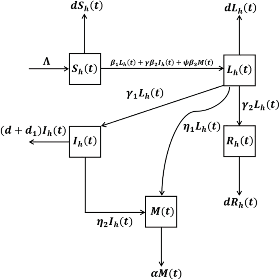
Figure 1: The graph describes the flowchart representing the transfer mechanism of the proposed epidemic problem
In the proposed problem,
Definition 2.1. [17] Let
and
In the above Eqs. (3) and (4), CF and C denote the Caputo-Fabrizio and Caputo. Moreover, t is positive, and
Definition 2.2. [17] If
is known as the Riemann-Liouville integral and
is said to be the Caputo-Fabrizio-Caputo (CF) integral.
Using the theory of fractional calculus to take the associated fractional version of the considered model. Since
To discuss the feasibility of the above epidemiological system (7) of fractional order, we discuss the existence as well as uniqueness analysis in the subsequent sections.
We exploit fixed point theory to show the model's existence and uniqueness under-considered, as Equation reported (7). We transform the reported system into its associated integral equations as
We apply the definition of CF integral, which ultimately implies that
Let us assume that
Theorem 2.1. The kernels
Proof 1. We assume that
Upon, the application of Cauchy's inequality leads to
We then obtain recursively the following relations:
The difference of two successive terms with the application of norm and majorizing, one may obtain
with
It could be noted that the kernels
Theorem 2.2. The epidemiological model of fractional order (7) possesses a solution.
Proof 2. From the assertions derived in Eq. (11) with the utilization of recursive formulas we obtain
So, the relations as described by the above equation are smooth and exists, however to investigate that the functions in these relations are the solutions for system (7), we making the substitutions
where
The application of norm on both sides of the above system with utilization of the Lipschitz axiom gives that
The application of
which completes the proof that solutions of the reported model described by Eq. (7) exists.
Theorem 2.3. The model reported by Eq. (7) posses a unique solution.
Proof 3. Let us assume that
Majorizing one may leads to the assertions as given by
We now use the result stated by Theorems 2.1 and 2.2, we obtain
For all n, the inequalities as reported by the above Eq. (19) holds, so
Now we are going to discuss the biological as well as mathematical feasibility of the problem under consideration. Notably, we discuss the positivity and boundedness of the reported model (7) to prove that the under-considered problem is well-possed. We also investigate that the dynamics of the proposed model are confined to a specific region that is invariant positively. The following Lemmas is established for this purpose.
Lemma 2.1. Since
Proof 4. We assume that,
where G represents the fractional operator having order is
where
Lemma 2.2. Let us assume that the
Proof 5. Let
Solving the above Eq. (24) which looks like
It could be also noted that
The solution of Eq. (26) leads to
In Eqs. (25) and (27), E(.) denote the Mittag-Leffler function and
We discuss the temporal dynamics of the considered model for the long run and present the significance of the fractional parameter. We find the numerical simulation to verify the theocratical work carried out for the fractional-order SARS-CoV-2 transmission epidemiological model (7). To show the validity of the analytical findings we present the large-scale simulation. There are not many choices like the traditional numerical methods to choose various schemes for the numerical simulation of fractional order models [46], therefore extensive attention is required to formulate new and convenient techniques for the simulation of fractional models. We follow a numerical scheme formulated in [47]. We assume the time step
Furthermore, we have chosen the value of epidemic parameters biologically as given in Table 1. We also assume the initial population sizes for various compartments of the proposed model as

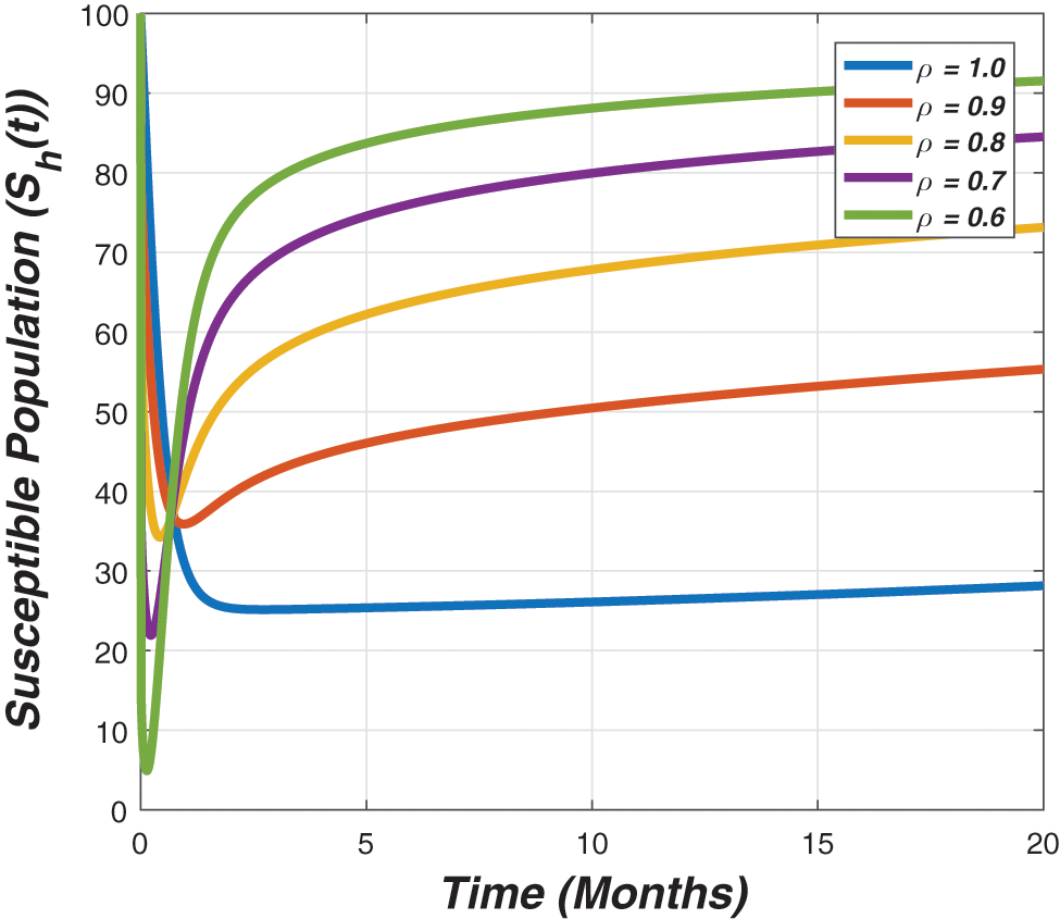
Figure 2: The graph visualizes the temporal dynamics of the susceptible for long run against various value of the fractional parameter (
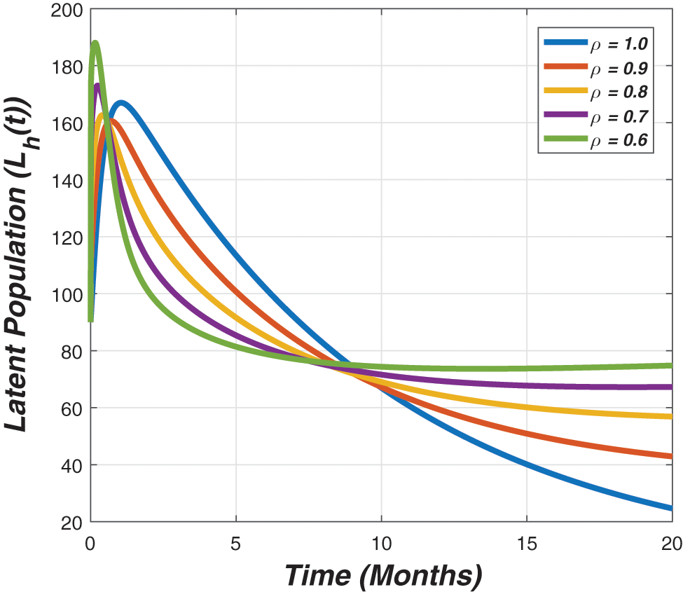
Figure 3: The plot demonstrate the dynamical behaviour of the latent individuals against the epidemic parameters value presented in Table 1 and different value of fractional parameter (
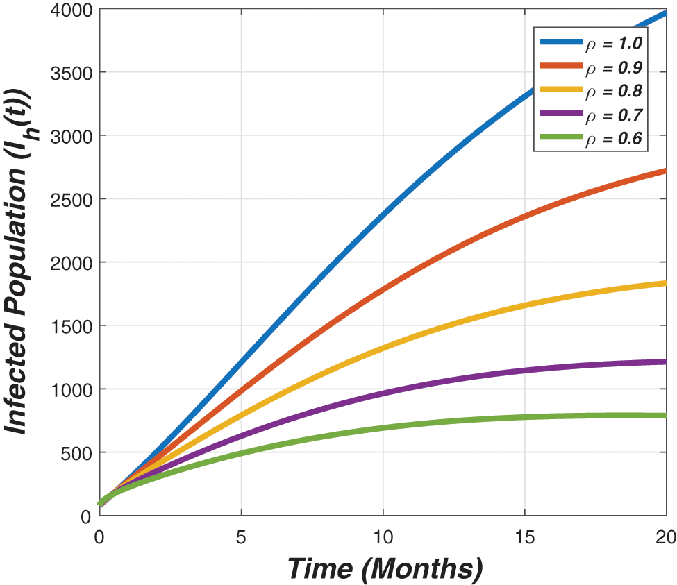
Figure 4: The graph represents the temporal dynamics of infected individuals against the fractional parameter (
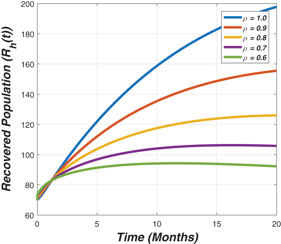
Figure 5: The graph describes the dynamics of the recovered individuals for different value of the fractional parameter (
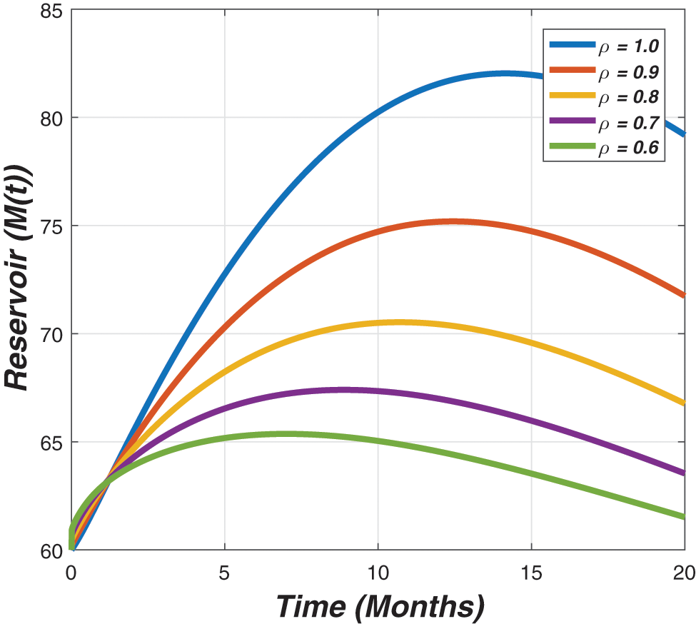
Figure 6: The graph describes the dynamics of the ratio of reservoir for different value of the fractional parameter (
We investigated the dynamics of SARS-CoV-2 with latent and infected individuals using an epidemic model. First, the formulation of the model is proposed and then consequently fractionalized due to the increased development in fractional calculus. Mainly, we used the well-known Caputo-Fabrizio operator for the said purposes, because this operator is based on the non-singular kernel and is more appropriate than the other fractional operator. Moreover, we applied the fixed point theorem to perform the existence analysis with unique properties regarding the developed epidemic problem. The biological and mathematical feasibilities are discussed in detail for the proposed model and prove that the problem is well-possed. Finally, we gave some graphical representations and showed the validations of the obtained results. We also presented the relative impact of the fractional parameter on the various groups of the compartmental populations graphically. We proved that the significant outcome of the reported work is that the fractional-order CF epidemic models are more appropriate and the best choice rather than the classical order.
In the near future, we will use the operators Atangana Baleanu Caputo, Atangana bi order, Atangana Gomez and fractal-fractional operator to study the complex dynamics of novel corona virus disease transmission. We will also apply the optimal control theory to the model reported in this study to present the control mechanism for the novel corona virus disease transmission.
Funding Statement: The author T. Abdeljawad would like to thank Prince Sultan University for the support through the TAS Research Lab and M. A. Alqudah was supported by Princess Nourah bint Abdulrahman University Researchers Supporting Project No. (PNURSP2022R14), Princess Nourah bint Abdulrahman University, Riyadh, Saudi Arabia.
Conflicts of Interest: The authors declare that they have no conflicts of interest to report regarding the present study.
References
1. Azhar, E. I., El-Kafrawy, S. A., Farraj, S. A., Hassan, A. M., Al-Saeed, M. S. et al. (2014). Evidence for camel-to-human transmission of mers coronavirus. New England Journal of Medicine, 370(26), 2499–2505. DOI 10.1056/NEJMoa1401505. [Google Scholar] [CrossRef]
2. Kim, Y., Lee, S., Chu, C., Choe, S., Hong, S. et al. (2016). The characteristics of Middle Eastern respiratory syndrome coronavirus transmission dynamics in South Korea. Osong Public Health and Research Perspectives, 7(1), 49–55. DOI 10.1016/j.phrp.2016.01.001. [Google Scholar] [CrossRef]
3. Al-Tawfiq, J. A., Hinedi, K., Ghandour, J., Khairalla, H., Musleh, S. et al. (2014). Middle East respiratory syndrome coronavirus: A case-control study of hospitalized patients. Clinical Infectious Diseases, 59(2), 160–165. DOI 10.1093/cid/ciu226. [Google Scholar] [CrossRef]
4. Chen, Z., Zhang, W., Lu, Y., Guo, C., Guo, Z. et al. (2020). From SARS-CoV to Wuhan 2019-nCoV outbreak: Similarity of early epidemic and prediction of future trends. CELL-HOST-MICROBE-D-20-00063. [Google Scholar]
5. Backer, J. A., Klinkenberg, D., Wallinga, J. (2020). Incubation period of 2019 novel coronavirus (2019-nCoV) infections among travellers from wuhan, China, 20–28 January 2020. Eurosurveillance, 25(5), 2000062. DOI 10.2807/1560-7917.ES.2020.25.5.2000062. [Google Scholar] [CrossRef]
6. Chen, S. B., Rashid, S., Noor, M. A., Ashraf, R., Chu, Y. M. (2020). A new approach on fractional calculus and probability density function. AIMS Mathematics, 5(6), 7041–7054. DOI 10.3934/math.2020451. [Google Scholar] [CrossRef]
7. Abdeljawad, T., Jarad, F., Atangana, A., Mohammed, P. O. (2020). On a new type of fractional difference operators on h-step isolated time scales: Weighted fractional difference operators. Journal of Fractional Calculus and Nonlinear Systems, 1(1), 46–74. DOI 10.48185/jfcns.v1i1.148. [Google Scholar] [CrossRef]
8. Chen, S. B., Jahanshahi, H., Abba, O. A., Solís-Pérez, J., Bekiros, S. et al. (2020). The effect of market confidence on a financial system from the perspective of fractional calculus: Numerical investigation and circuit realization. Chaos, Solitons & Fractals, 140, 110223. DOI 10.1016/j.chaos.2020.110223. [Google Scholar] [CrossRef]
9. Al-Mdallal, Q. M., Hajji, M. A., Abdeljawad, T. (2021). On the iterative methods for solving fractional initial value problems: New perspective. Journal of Fractional Calculus and Nonlinear Systems, 2(1), 76–81. DOI 10.48185/jfcns.v2i1.297. [Google Scholar] [CrossRef]
10. Ziada, E. (2021). Numerical solution for multi-term fractional delay differential equations. Journal of Fractional Calculus and Nonlinear Systems, 2(2), 1–12. DOI 10.48185/jfcns.v2i2.358. [Google Scholar] [CrossRef]
11. Abdeljawad, T., Suwan, I., Jarad, F., Qarariyah, A. (2021). More properties of fractional proportional differences. Journal of Mathematical Analysis and Modeling, 2(1), 72–90. DOI 10.48185/jmam.v2i1.193. [Google Scholar] [CrossRef]
12. Rashid, S., Sultana, S., Karaca, Y., Khalid, A., Chu, Y. M. (2021). Some further extensions considering discrete proportional fractional operators. Fractals, 30, 2240026. [Google Scholar]
13. Atangana, A. (2020). Modelling the spread of COVID-19 with new fractal-fractional operators: Can the lockdown save mankind before vaccination? Chaos, Solitons & Fractals, 136, 109860. DOI 10.1016/j.chaos.2020.109860. [Google Scholar] [CrossRef]
14. Atangana, A., Araz, S. I. (2021). Nonlinear equations with global differential and integral operators: Existence, uniqueness with application to epidemiology. Results in Physics, 20, 103593. DOI 10.1016/j.rinp.2020.103593. [Google Scholar] [CrossRef]
15. Haidong, Q., Arfan, M., Salimi, M., Salahshour, S., Ahmadian, A. et al. (2021). Fractal–fractional dynamical system of typhoid disease including protection from infection. Engineering with Computers, 2021, 1–10. DOI 10.1007/s00366-021-01536-y. [Google Scholar] [CrossRef]
16. Samko, S. G. (1987). Fractional integrals and derivatives, theory and applications. Minsk: Nauka I Tekhnika. [Google Scholar]
17. Baleanu, D., Güvenç, Z. B., Machado, J. T. (2010). New trends in nanotechnology and fractional calculus applications. New York: Springer. [Google Scholar]
18. Baleanu, D., Machado, J. A. T., Luo, A. C. (2011). Fractional dynamics and control. Springer Science & Business Media. [Google Scholar]
19. Baleanu, D., Diethelm, K., Scalas, E., Trujillo, J. J. (2012). Fractional calculus: Models and numerical methods, vol. 3. World Scientific, Singapore. [Google Scholar]
20. Ali, N., Zaman, G., Zeb, A., Erturk, V. S., Jung, I. H. et al. (2019). Dynamical analysis of approximate solutions of HIV-1 model with an arbitrary order. Complexity, 7. [Google Scholar]
21. Zafar, Z. U. A., Ali, N., Baleanu, D. (2021). Dynamics and numerical investigations of a fractional-order model of toxoplasmosis in the population of human and cats. Chaos, Solitons & Fractals, 151, 111261. DOI 10.1016/j.chaos.2021.111261. [Google Scholar] [CrossRef]
22. Zafar, Z. U. A., Shah, Z., Ali, N., Alzahrani, E. O., Shutaywi, M. (2021). Mathematical and stability analysis of fractional order model for spread of pests in tea plants. Fractals, 29(1), 2150008. DOI 10.1142/S0218348X21500080. [Google Scholar] [CrossRef]
23. Srivastava, H. M., Saad, K. M., Gómez-Aguilar, J., Almadiy, A. A. (2020). Some new mathematical models of the fractional-order system of human immune against iav infection. Mathematical Biosciences and Engineering, 17(5), 4942–4969. DOI 10.3934/mbe.2020268. [Google Scholar] [CrossRef]
24. Tuan, N. H., Mohammadi, H., Rezapour, S. (2020). A mathematical model for COVID-19 transmission by using the caputo fractional derivative. Chaos, Solitons & Fractals, 140, 110107. DOI 10.1016/j.chaos.2020.110107. [Google Scholar] [CrossRef]
25. Owolabi, K. M., Atangana, A. (2017). Numerical approximation of nonlinear fractional parabolic differential equations with caputo–fabrizio derivative in riemann–liouville sense. Chaos, Solitons & Fractals, 99, 171–179. DOI 10.1016/j.chaos.2017.04.008. [Google Scholar] [CrossRef]
26. Baleanu, D., Jajarmi, A., Hajipour, M. (2018). On the nonlinear dynamical systems within the generalized fractional derivatives with mittag–leffler kernel. Nonlinear Dynamics, 94(1), 397–414. DOI 10.1007/s11071-018-4367-y. [Google Scholar] [CrossRef]
27. Baleanu, D., Mohammadi, H., Rezapour, S. (2020). Analysis of the model of HIV-1 infection of CD4+ T-cell with a new approach of fractional derivative. Advances in Difference Equations, 2020(1), 1–17. DOI 10.1186/s13662-020-02544-w. [Google Scholar] [CrossRef]
28. Caputo, M., Fabrizio, M. (2015). A new definition of fractional derivative without singular kernel. Progress in Fractional Differentiation & Applications, 1(2), 73–85. [Google Scholar]
29. Rihan, F., Al-Mdallal, Q., AlSakaji, H., Hashish, A. (2019). A fractional-order epidemic model with time-delay and nonlinear incidence rate. Chaos, Solitons & Fractals, 126, 97–105. DOI 10.1016/j.chaos.2019.05.039. [Google Scholar] [CrossRef]
30. Li, X. P., Al Bayatti, H., Din, A., Zeb, A. (2021). A vigorous study of fractional order COVID-19 model via abc derivatives. Results in Physics, 29, 104737. DOI 10.1016/j.rinp.2021.104737. [Google Scholar] [CrossRef]
31. Li, X. P., Wang, Y., Khan, M. A., Alshahrani, M. Y., Muhammad, T. (2021). A dynamical study of SARS-COV-2: A study of third wave. Results in Physics, 29, 104705. DOI 10.1016/j.rinp.2021.104705. [Google Scholar] [CrossRef]
32. Li, X. P., Gul, N., Khan, M. A., Bilal, R., Ali, A. et al. (2021). A new hepatitis b model in light of asymptomatic carriers and vaccination study through atangana–baleanu derivative. Results in Physics, 29, 104603. DOI 10.1016/j.rinp.2021.104603. [Google Scholar] [CrossRef]
33. Chen, S. B., Soradi-Zeid, S., Jahanshahi, H., Alcaraz, R., Gómez-Aguilar, J. F. et al. (2020). Optimal control of time-delay fractional equations via a joint application of radial basis functions and collocation method. Entropy, 22(11), 1213. DOI 10.3390/e22111213. [Google Scholar] [CrossRef]
34. Chen, S. B., Rajaee, F., Yousefpour, A., Alcaraz, R., Chu, Y. M. et al. (2021). Antiretroviral therapy of hiv infection using a novel optimal type-2 fuzzy control strategy. Alexandria Engineering Journal, 60(1), 1545–1555. DOI 10.1016/j.aej.2020.11.009. [Google Scholar] [CrossRef]
35. Shen, Z. H., Chu, Y. M., Khan, M. A., Muhammad, S., Al-Hartomy, O. A. et al. (2021). Mathematical modeling and optimal control of the COVID-19 dynamics. Results in Physics, 31, 105028. DOI 10.1016/j.rinp.2021.105028. [Google Scholar] [CrossRef]
36. Jain, S., El-Khatib, Y. (2021). Stochastic COVID-19 model with fractional global and classical piecewise derivative. Results in Physics, 30, 104788. DOI 10.1016/j.rinp.2021.104788. [Google Scholar] [CrossRef]
37. Shafiq, A., Lone, S., Sindhu, T. N., El Khatib, Y., Al-Mdallal, Q. M. et al. (2021). A new modified kies fréchet distribution: Applications of mortality rate of COVID-19. Results in Physics, 28, 104638. DOI 10.1016/j.rinp.2021.104638. [Google Scholar] [CrossRef]
38. Rihan, F., Alsakaji, H. (2021). Dynamics of a stochastic delay differential model for COVID-19 infection with asymptomatic infected and interacting people: Case study in the uae. Results in Physics, 28, 104658. DOI 10.1016/j.rinp.2021.104658. [Google Scholar] [CrossRef]
39. Wu, J. T., Leung, K., Leung, G. M. (2020). Nowcasting and forecasting the potential domestic and international spread of the 2019-nCoV outbreak originating in Wuhan, China: A modelling study. The Lancet, 395(10225), 689–697. DOI 10.1016/S0140-6736(20)30260-9. [Google Scholar] [CrossRef]
40. Imai, N., Cori, A., Dorigatti, I., Baguelin, M., Donnelly, C. A. et al. (2020). Report 3: Transmissibility of 2019-nCoV. Imperial College London. [Google Scholar]
41. Zhu, H., Guo, Q., Li, M., Wang, C., Fang, Z. et al. (2020). Host and infectivity prediction of Wuhan 2019 novel coronavirus using deep learning algorithm. Cold Spring Harbor Laboratory. [Google Scholar]
42. Rothe, C., Schunk, M., Sothmann, P., Bretzel, G., Froeschl, G. et al. (2020). Transmission of 2019-nCoV infection from an asymptomatic contact in Germany. New England Journal of Medicine, 970–971. DOI 10.1056/NEJMc2001468. [Google Scholar] [CrossRef]
43. Read, J. M., Bridgen, J. R., Cummings, D. A., Ho, A., Jewell, C. P. (2020). Novel coronavirus 2019-nCoV: Early estimation of epidemiological parameters and epidemic predictions. Cold Spring Harbor Laboratory Press. [Google Scholar]
44. Li, W., Deng, X., Shao, H., Wang, X. (2021). Deep learning applications for COVID-19 analysis: A state-of-the-art survey. Computer Modeling in Engineering & Sciences, 129(1), 65–98. DOI 10.32604/cmes.2021.016981. [Google Scholar] [CrossRef]
45. Yang, X., Chen, L., Chen, J. (1996). Permanence and positive periodic solution for the single-species nonautonomous delay diffusive models. Computers & Mathematics with Applications, 32(4), 109–116. DOI 10.1016/0898-1221(96)00129-0. [Google Scholar] [CrossRef]
46. Ramos, H., Kalogiratou, Z., Monovasilis, T., Simos, T. (2016). An optimized two-step hybrid block method for solving general second order initial-value problems. Numerical Algorithms, 72(4), 1089–1102. DOI 10.1007/s11075-015-0081-8. [Google Scholar] [CrossRef]
47. Li, C., Zeng, F. (2019). Numerical methods for fractional calculus. Chapman and Hall/CRC. [Google Scholar]
Cite This Article
 Copyright © 2023 The Author(s). Published by Tech Science Press.
This work is licensed under a Creative Commons Attribution 4.0 International License , which permits unrestricted use, distribution, and reproduction in any medium, provided the original work is properly cited.
 Downloads
 Citation Tools