Numerical Simulation of the Fractional-Order Lorenz Chaotic Systems with Caputo Fractional Derivative

1  Introduction

In 1963, Edward Lorenz discovered a mathematical model for atmospheric convection. This model is also known as Lorenz chaotic system. The Lorenz system is widely used in electric circuits, forward osmosis and chemical reactions. In recent years, people have studied the chaotic behavior in the fractional dynamic system and found that the fractional dynamic system has unique properties that the integer dynamic system does not have. Therefore, the numerical simulation of fractional chaotic system is very important. In this paper, we simulate the fractional-order Lorenz chaotic dynamical systems [1–6] is as

{Dtα1x(t)=σ(y(t)−x(t)),Dtα2y(t)=ρx(t)−y(t)−x(t)z(t),t∈[0,T],Dtα3z(t)=x(t)y(t)−βz(t),(1)

with the initial conditions

x(0)=c1,y(0)=c2,z(0)=c3.(2)

The solutions of the fractional-order Lorenz chaotic dynamical systems are very hard to obtain analytically, and researchers, therefore, rely on numerical methods to provide an approximate solution that could be used for prediction. In the last decades, several numerical methods have been proposed. In [1], based on the qualitative theory, the authors investigated the existence and uniqueness of solutions for a class of fractional-order Lorenz chaotic systems (1). In [2], compared the dynamical regimes of fractional-order systems with dynamical regimes of the corresponding standard systems. In [3], Complex dynamics with interesting characteristics were presented by means of phase portraits, the largest Lyapunov exponent and bifurcation diagrams. In [4–6], the authors gave a dynamic analysis of a fractional-order Lorenz chaotic system. Although some numerical and analytical methods of the FDEs have been announced, such as spectral method [7–11], reproducing kernel method [12–19], homotopy perturbation method [20–23], high-precision numerical approach [24–27], and so on numerical and analytical methods [28–36]. These researchers all say their own approach can accurately simulate chaotic systems. In fact, since chaotic systems have no exact solution, researchers do not know which method is more accurate. For the numerical simulation of chaotic systems, it is necessary to use numerical methods to study the long time properties of solutions of the fractional order chaotic systems. This paper introduces a high-precision numerical method [24–27] for solving system (1). Some complex dynamic behavior of the fractional-order Lorenz chaotic systems are discovered by using the present numerical approach. We observe some novel dynamic behavior in numerical simulations which are unlike any that have been previously discovered in numerical simulations or theoretical studies. The simulation results of numerical experiments demonstrate the effectiveness of the present method.

Fractal and fractional calculus [37–48] have been widely concerned. In the last three decades, there have existed many inequivalent definitions [49–51] of fractional derivatives. The most famous of these definitions that have been widely popularized in the world of fractional calculus is Riemann-Liouville fractional definition, Gru¨nwald-Letnikov fractional derivative (GLFD) and Caputo fractional derivative definition.

Definition 1.1. Riemann-Liouville fractional derivative of order α of a function y(t) about t on the interval (t0,t) is defined as

t0RLDtαy(t)={1Γ(n−α)dndtn∫t0ty(τ)(t−τ)α−n+1dτ,0≤n−1<α<n.dny(t)dtn,α=n∈N.(3)

Definition 1.2. Caputo fractional derivative of order α of a function y(t)∈Cn[t0,t] about t on the interval (t0,t) is defined as

t0CDtαy(t)={1Γ(n−α)∫t0ty(n)(τ)(t−τ)α−n+1dτ,0≤n−1<α<n.dny(t)dtn,α=n∈N.(4)

Definition 1.3. The Gru¨nwald-Letnikov fractional derivative of α-order on the interval (t0,t) is defined as

t0GLDtαy(t)=limh→01hα∑j=0[(t−t0)/h]⁡(−1)j(jα)y(t−jh),(5)

where

(−1)j(jα)=(−1)jΓ(α+1)Γ(j+1)Γ(α−j+1).

Let

ωj(α)=(−1)j(jα)=(−1)jΓ(α+1)Γ(j+1)Γ(α−j+1),j=0,1,…,n.(6)

Therefore, the α-order Gru¨nwald-Letnikov derivative in Eq. (4) is transformed into the following form:

t0GLDtαy(t)=limh→01hα∑j=0[(t−t0)/h]⁡ωj(α)y(t−jh).(7)

Using Newton’s binomial theorem, we know

(1−z)n=∑j=0n⁡(−1)j(jn)zj=∑j=0n⁡ωj(n)zj.(8)

We can proof the following form:

∑j=0∞⁡ωj(α)zj=(1−z)α.(9)

(1−z)α is called 1-order generating function of α-order Gru¨nwald-Letnikov derivative on the interval (t0,t).

t0GLDtαy(t)=1hα∑i=0[(t−t0)/h]⁡ωjy(t−ih)+o(h).(10)

Theorem 1.4. If f(t) is continuous and differentiable of order n−1 on the interval (t0,t), and f(n)(t) is integrable, then Gru¨nwald-Letnikov derivative can be written in the following integral form:

t0GLDtαy(t)=∑j=0n−1⁡y(j)(t0)Γ(1+j−α)(t−t0)j−α+1Γ(n−α)∫0ty(n)(τ)(t−τ)α−n+1dτ,0≤n−1<α<n.(11)

and, the Gru¨nwald-Letnikov derivative, Riemann-Liouville derivative and Caputo derivative have the following relationship:

t0GLDtαy(t)=t0RLDtαy(t),t0CDtαy(t)=t0RLDtαy(t)−∑j=0n−1⁡y(j)(t0)Γ(1+j−α)(t−t0)j−α.(12)

Proof 1. For the proof, please refer to [49].

From Theorem (1.4), it follows that, if y(j)(t0)=0,j=0,1,…,n−1, then t0GLDtαy(t)=t0RLDtαy(t)=t0CDtαy(t). If exists j, such that y(j)(t0)≠0,j=0,1,…,n−1, we use Taylor form, let y¯(t)=y(t)−∑j=0n−1y(j)(t0)Γ(1+j−α)(t−t0)j−α, then t0GLDtαy¯(t)=t0RLDtαy¯(t)=t0CDtαy¯(t). For convenience of expression, we denote

t0GLDtαy(t)=t0RLDtαy(t)=t0CDtαy(t)=Dtαy(t).

2  Numerical Approach

In [24–27], in order to obtain higher precision, author given the construction method of generating function for arbitrary p, and then give a recursive method of fractional derivative and integral based on the generating function.

Definition 2.1. A p-order polynomial function is defined as

gp(z)=∑k=1p⁡1k(1−z)k.(13)

Theorem 2.2. The p order polynomial function gp(z) could be written as

gp(z)=∑k=0p⁡gkzk,(14)

where gk is the solutions of the following equation [24–27]:

(111⋯1123⋯p+112232⋯(p+1)2⋮⋮⋮⋯⋮12p3p⋯(p+1)p)(g0g1g2⋮gp)=−(012⋮p).(15)

Proof 2. It can be seen from Eqs. (13) and (14)

∑k=0p⁡gkzk=∑k=1p⁡1k(1−z)k.(16)

Substituting z=1 into Eq. (16), there is

∑k=0p⁡gk=0.(17)

Multiply both ends of Eq. (16) by z and find the first derivative of z, then

∑k=0p⁡(k+1)gkzk=∑k=1p⁡1k(1−z)k−z∑k=1p⁡(1−z)k−1.(18)

Then substitute z=1 into Eq. (18), then there is

∑k=0p⁡(k+1)gk=−1.

Multiply both ends of Eq. (16) by z, and then find the first derivative of z

∑k=0p⁡(k+1)2gkzk=∑k=1p⁡1k(1−z)k−3z∑k=1p⁡(1−z)k−1+z2∑k=2p⁡1k−1(1−z)k−2.(19)

Substituting z=1 into Eq. (19), we can derive

∑k=0p⁡(k+1)2gk=−2.

Repeating the above process, the following equation can be established:

{g0+g1+g2+⋯+gp=0,g0+2g1+3g2+⋯+(p+1)gp=−1,g0+22g1+32g2+⋯+(p+1)2gp=−2,⋮g0+2pg1+3pg2+⋯+(p+1)pgp=−p.

The matrix form of the equation is formula (15), which is proved by the theorem.

Definition 2.3. Ihe p-order generating function gpα(z) of α-order Gru¨nwald-Letnikov derivative is defined as

gpα(z)=(g0+g1z+⋯+gpzp)α.(20)

Theorem 2.4. If the generating function gpα(z) can be written as

gpα(z)=∑k=0∞⁡ωk(α,p)zk.(21)

where the subsequent coefficient ω(α,p)k can be recursively calculated by the following formula [24–27]:

{ωk(α,p)=g0α,k=0,ωk(α,p)=−1g0∑i=1p⁡gi(1−i1+αk)ωk−i(α,p),k=1,2,…,ωk(α,p)=0,k<0.(22)

Proof 3. Let z=0 in Eq. (20), then it can be proved ω0(α,p)=g0α. Rewritten Eq. (20), it can be seen that

(g0+g1z+⋯+gpzp)α=∑k=−∞∞⁡ωk(α,p)zk,(23)

where, if k<0, then ωk(α,p)=0. Find the first derivative of z on both sides of Eq. (23), it can be concluded that

α(g1+2g2z+⋯+pgpzp−1)(g0+g1z+⋯+gpzp)α−1=∑k=−∞∞⁡kωk(α,p)zk−1.(24)

Both sides of Eq. (24) are multiplied by (g0+g2z+⋯+gpzp) at the same time, it can be seen

α(g1+⋯+pgpzp−1)(g0+⋯+gpzp)α=(g0+⋯+gpzp)∑k=−∞∞⁡kωk(α,p)zk−1.(25)

Substituting Eq. (23) into Eq. (25), we can get

α(g1+⋯+pgpzp−1)∑k=−∞∞⁡ωk(α,p)zk=(g0+⋯+gpzp)∑k=−∞∞⁡kωk(α,p)zk−1.(26)

Using the zdωk(α,p)=ωk−d(α,p) property, the left end of Eq. (26) can be written as

∑k=−∞∞⁡α(g1ωk(α,p)+2g2ωk−1(α,p)+⋯+pgpωk−p+1(α,p))zk,(27)

then its right end can be written

∑k=−∞∞⁡[(k+1)g0ωk+1(α,p)+kg1ωk(α,p)+⋯+(k−p+1)gpωk−p+1(α,p)]zk.(28)

By comparing the same square coefficient of z in Eq. (27), we can get

α(g1ωk(α,p)+⋯+pgpωk−p+1(α,p))=(k+1)g0ωk+1(α,p)+⋯+(k−p+1)gpωk−p+1(α,p).(29)

Move Eq. (29) back one step, let k=k−1, then the equation can become

g0kωk(α,p)+g1(k−1−α)ωk−1(α,p)+⋯+gp(k−p−pα)ωk−p(α,p)=0.(30)

If k≠0, it is thus clear that

ωk(α,p)=−1g0[g1(1−1+αk)ωk−1(α,p)+g2(1−21+αk)ωk−2(α,p)+⋯+gp(1−p1+αk)ωk−p(α,p)](31)

where, when k<0, ωk(α,p)=0.The above formula is recursive, so the theorem is proved.

Corollary 2.5. The p-order generating function gpα(z) of α-order Gru¨nwald-Letnikov derivative could be written as [24–27]

gpα(z)=∑j=0∞⁡ωj(α,p)zj.(32)

where

{ωk(α,p)=g0,k=0,ωk(α,p)=−1g0∑i=0k−1⁡(1−i1+αk)giωk−i(α,p),k=1,2,….,p−1,ωk(α,p)=−1g0∑i=0p⁡(1−i1+αk)giωk−i(α,p),k=p,p+1,p+2,….,ωk(α,p)=0,k<0,(33)

The α-order Gru¨nwald-Letnikov fractional derivative with p-order generating function gpα(z) is given as

t0GLDtαy(t)=limh→01hα∑i=0[(t−t0)/h]⁡ωi(α,p)y(t−ih).(34)

Applying (34), an approximate computation scheme of the α-order Caputo fractional derivative with p-order generating function gpα(z) is given as

Dtαy(t)≃ym=1hα∑j=0m⁡ωj(α,p)y(t−jh)=1hαy(tk)−1hα∑i=1m⁡ωj(α,p)y(tk−j).(35)

and limm→∞ym=Dtαy(t).

So, a high-precision numerical approach of the fractional-order Lorenz chaotic systems (1) is given by

{x(tk)=σhα1(y(tk−1)−x(tk))+x(0)−∑j=1m⁡ωj(α1,p)(x(tk−j)−x(0)),y(tk)=hα2(ρx(tk)−y(tk−1)−x(tk)z(tk−1))+y(0)−∑j=1m⁡ωj(α2,p)(y(tk−j)−y(0)),z(tk)=hα3(x(tk)y(tk)−βz(tk−1))+z(0)−∑j=1m⁡ωj(α3,p)(z(tk−j)−z(0)).(36)

3  Numerical Experiment

In this section, some numerical examples are studied. Some novel chaotic behaviors are shown. We consider the systems (1) with the initial conditions x(0)=−15,y(0)=−15,z(0)=20. h=0.01,p=20. The complex dynamic behaviors of the systems (1) are shown in Figs. 1–21. Fig. 1 shows time series plots of the systems (1) with parameters [σ,ρ,β]=[10,28,8/3] at different α. Figs. 2 and 3 show time series plots of the systems (1) with different parameters [σ,ρ,β] and different fractional derivative α. Figs. 4–19 projected on the (x,y), (x,z), (y,z)-plane and show phase diagram of x, y, z of the systems (1) with different parameters [σ,ρ,β] and different fractional derivative α. Figs. 20 and 21 show chaotic attractor of fractional-order Lorenz systems (1) with different parameters [σ,ρ,β] and different fractional derivative α. The rich chaotic attractor of fractional-order Lorenz systems (1) is shown in Figs. 20 and 21. The simulation results of integer order are in good agreement with those of other methods. In this paper, many novel chaotic attractors for fractional systems are obtained.

Figure 1: Time series plots of the systems (1) at [σ,ρ,β]=[10,28,8/3] with parameters α

Figure 2: Time series plots of the systems (1) with different parameters

Figure 3: Numerical results for the systems (1) at α=[1.16,1.18,1.15],[σ,ρ,β]=[35,20,15], T=100

Figure 4: Numerical results for the systems (1) at α=[0.9,1.29,1.28],[σ,ρ,β]=[8,12,10], T=100

Figure 5: Numerical results for the systems (1) at α=[1.29,1.2,1.1],[σ,ρ,β]=[8,12,10], T=100

Figure 6: Numerical results for the systems (1) at α=[0.95,1.02,1.03],[σ,ρ,β]=[10,28,8/3], T=100

Figure 7: Numerical results for the systems (1) at α=[1.1,1.15,1.18],[σ,ρ,β]=[10,28,8/3], T=100

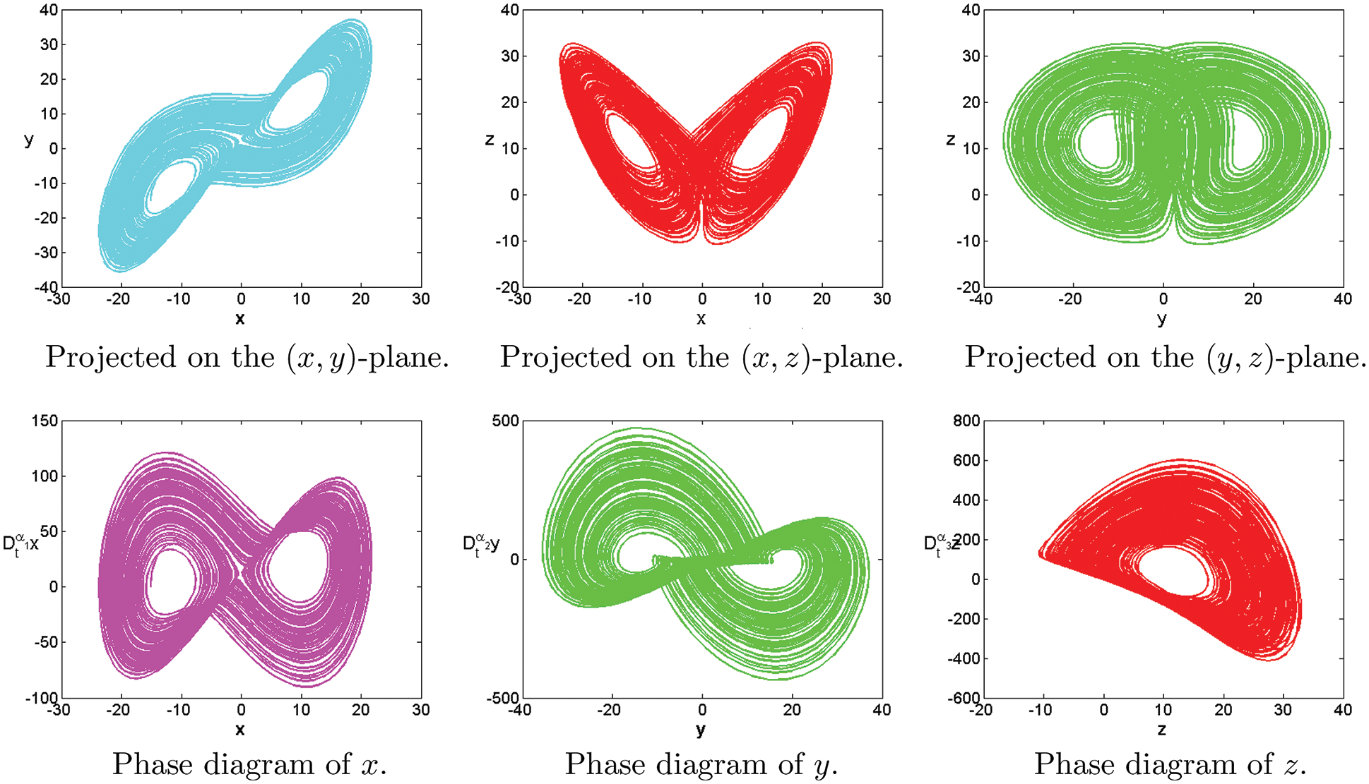
Figure 8: Numerical results for the systems (1) at α=[0.9,1.02,1.27],[σ,ρ,β]=[5,12,10], T=100

Figure 9: Numerical results for the systems (1) at α=[0.9,1.18,1.38],[σ,ρ,β]=[3,10,11], T=100

Figure 10: Numerical results for the systems (1) at α=[1,1.18,1.38],[σ,ρ,β]=[1,8,15], T=100

Figure 11: Numerical results for the systems (1) at α=[1.22,2.21,1.19],[σ,ρ,β]=[20,10,9]

Figure 12: Numerical results for the systems (1) at α=[1,1.12,1.18],[σ,ρ,β]=[4,9,9], T=100

Figure 13: Numerical results for the systems (1) at α=[1,1.12,1.18],[σ,ρ,β]=[6,8,9], T=100

Figure 14: Numerical results for the systems (1) at α=[1,0.98,1.15],[σ,ρ,β]=[15,20,10], T=100

Figure 15: Numerical results for the systems (1) at α=[1.12,1.26,1.28],[σ,ρ,β]=[30,30,10], T=100

Figure 16: Numerical results for (1) at α=[1.35,1.25,1.2],[c1,c2,c3]=[−18,−25,20],[σ,ρ,β]=[35,15,9], T=100

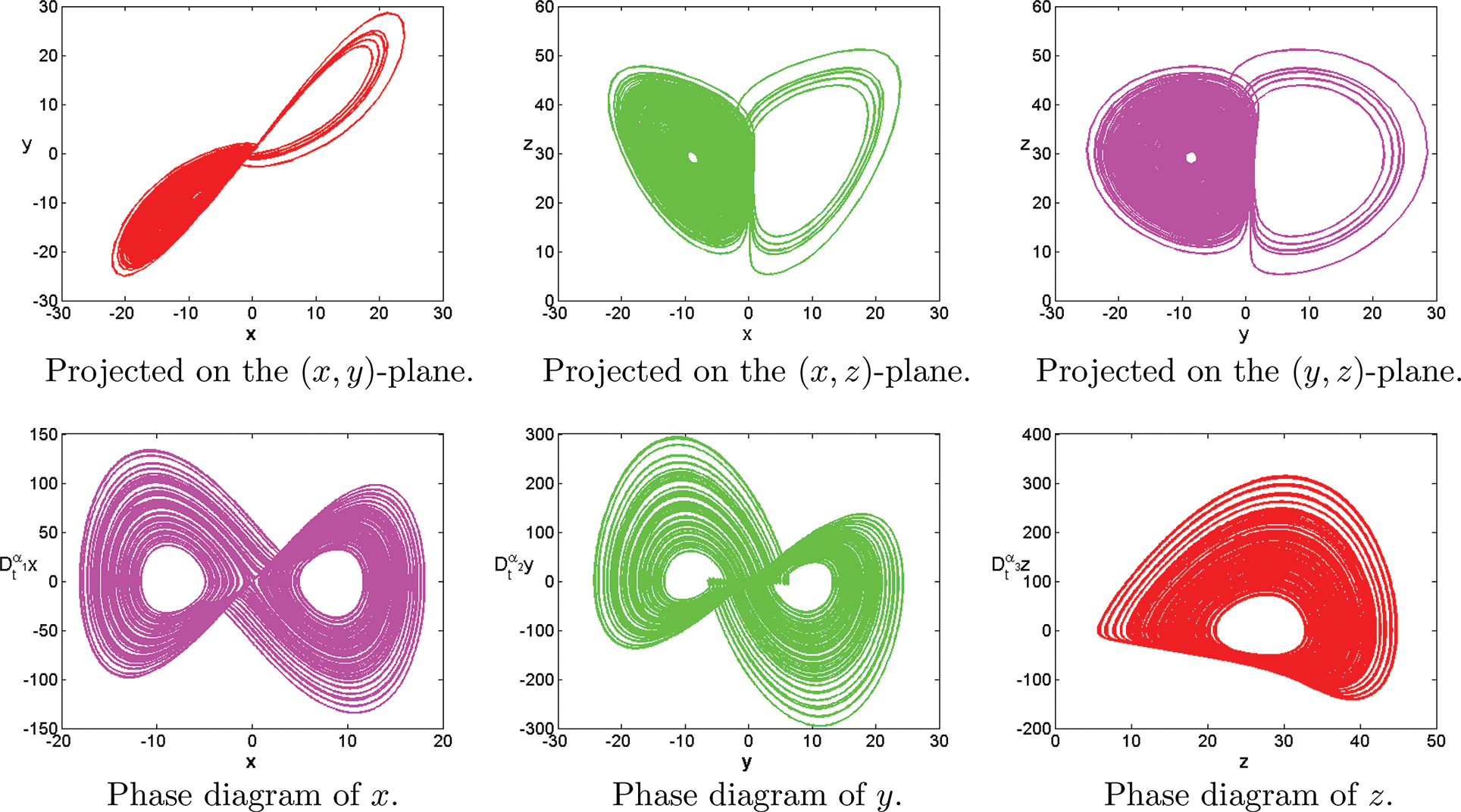
Figure 17: Numerical results for the systems (1) at α=[0.92,0.99,1.01],[σ,ρ,β]=[20,30,8/3], T=100

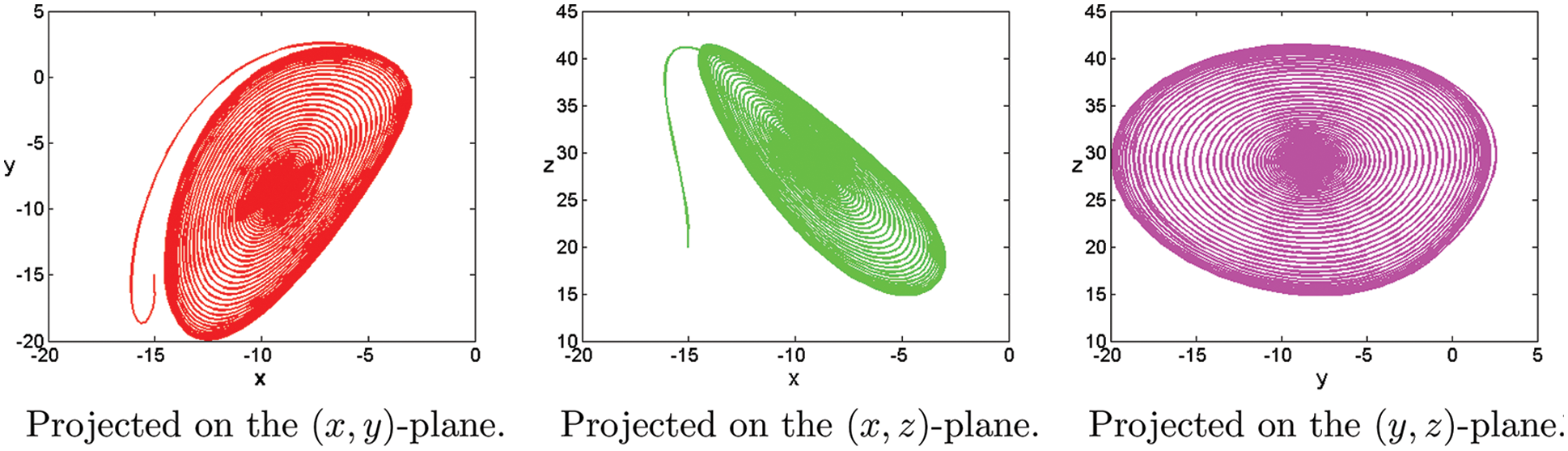
Figure 18: Numerical results for the systems (1) at α=[0.92,1,1],[σ,ρ,β]=[5,30,8/3], T=100

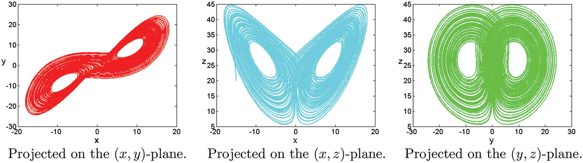
Figure 19: Numerical results for the systems (1) at α=[1,1,1],[σ,ρ,β]=[10,28,8/3], T=100

Figure 20: Chaotic attractor of fractional-order Lorenz systems (1) with different parameters

Figure 21: Chaotic attractor of fractional-order Lorenz systems (1) with different parameters

4  Conclusions and Remarks

In this paper, some complex dynamic behavior of fractional-order Lorenz chaotic systems are shown by using the present method. We observe many novel dynamic behaviors in numerical experiments which are unlike any that have been previously discovered in numerical experiments or theoretical studies. We investigate the influence of α1, α2, α3 on the numerical solution of fractional-order Lorenz chaotic systems. The simulation results of integer order are in good agreement with those of other methods. The results presented in this paper suggested that the present numerical method is also readily applicable to a more chaotic system.

All computations are performed by the MatlabR2017b software.

Acknowledgement: The authors would like to express their thanks to the unknown referees for their careful reading and helpful comments.

Funding Statement: This paper is supported by the Natural Science Foundation of Inner Mongolia [2021MS01009] and Jining Normal University [JSJY2021040, Jsbsjj1704, jsky202145].

Conflicts of Interest: The authors declare that they have no conflicts of interest to report regarding the present study.

References

1. Yu, Y. G., Li, H. X., Wang, S., Yu, J. Z. (2009). Dynamic analysis of a fractional-order lorenz chaotic system. Chaos Solitons & Fractals, 42(2), 1181–1189. DOI 10.1016/j.chaos.2009.03.016. [Google Scholar] [CrossRef]
2. Letellier, C., Aguirre, L. A. (2013). Dynamical analysis of fractional-order rossler and modified lorenz systems. Physics Letters Section A General Atomic Solid State Physics, 377(28–30), 1707–1719. [Google Scholar]
3. Sun, K., Wang, X., Sprott, J. C. (2010). Bifurcations and chaos in fractional-order simplified lorenz system. International Journal of Bifurcation and Chaos, 20(4), 1209–1219. DOI 10.1142/S0218127410026411. [Google Scholar] [CrossRef]
4. Qiao, W. (2013). Chaos control in the fractional-order lorenz system with random parameter. Applied Mechanics and Materials, 278–280, 1423–1426. DOI 10.4028/www.scientific.net/AMM.278-280.1423. [Google Scholar] [CrossRef]
5. Grigorenko, I., Grigorenko, E. (2003). Chaotic dynamics of the fractional lorenz system. Physical Review Letters, 91(3), 034101. DOI 10.1103/PhysRevLett.91.034101. [Google Scholar] [CrossRef]
6. Wang, X. Y., Song, J. M. (2009). Synchronization of the fractional order hyperchaos Lorenz systems with activation feedback control. Communications in Nonlinear Science and Numerical Simulation, 14(8), 3351–3357. DOI 10.1016/j.cnsns.2009.01.010. [Google Scholar] [CrossRef]
7. Han, C., Wang, Y. L., Li, Z. Y. (2022). A high-precision numerical approach to solving space fractional gray-scott model. Applied Mathematics Letters, 125, 107759. DOI 10.1016/j.aml.2021.107759. [Google Scholar] [CrossRef]
8. Zhang, X. L., Zhang, W., Wang, Y. L., Ban, T. T. (2021). The space spectral interpolation collocation method for reaction-diflusion systems. Thermal Science, 25(2B), 269–1275. [Google Scholar]
9. Li, X. Y., Han, C., Wang, Y. L. (2022). Novel patterns in fractional-in-space nonlinear coupled FitzHugh–Nagumo models with riesz fractional derivative. Fractal and Fractional, 6(3), 136. DOI 10.3390/fractalfract6030136. [Google Scholar] [CrossRef]
10. Han, C., Wang, Y. L. (2022). Numerical solutions of variable-coefficient fractional-in-space KdV equation with the caputo fractional derivative. Fractal and Fractional, 6(4), 207. DOI 10.3390/fractalfract6040207. [Google Scholar] [CrossRef]
11. Han, C., Wang, Y. L., Li, Z. Y. (2021). Numerical solutions of space fractional variable-coefficient KdV-modified KdV equation by Fourier spectral method. Fractals, 29(8), 2150246. DOI 10.1142/S0218348X21502467. [Google Scholar] [CrossRef]
12. Wang, Y. L., Tian, D., Bao, S. H., Li, Z. Y. (2017). Using the iterative reproducing kernel method for solving a class of nonlinear fractional differential equations. International Journal of Computer Mathematics, 12(94), 2558–2572. [Google Scholar]
13. Wang, Y. L., Jia, L. N., Zhang, H. L. (2019). Numerical solution for a class of space-time fractional equation by the piecewise reproducing kernel method. International Journal of Computer Mathematics, 96(10), 2100–2111. DOI 10.1080/00207160.2018.1544367. [Google Scholar] [CrossRef]
14. Zhang, W., Wang, Y. L., Wang, M. C. (2020). Using reproducing kernel for solving a class of the time variable fractional order reaction-diflusion model. Thermal Science, 24(4), 2553–2559. DOI 10.2298/TSCI2004553Z. [Google Scholar] [CrossRef]
15. Dai, D. D., Ban, T. T., Wang, Y. L., Zhang, W. (2021). The piecewise reproducing kernel method for the time variable fractional order advection-reaction-diflusion equations. Thermal Science, 25, 1261–1268. [Google Scholar]
16. Wang, Y. L., Chaolu, T., Pang, J. (2009). New algorithm for second-order boundary value problems of integro-differential equation. Journal of Computational and Applied Mathematics, 229(1), 1–6. DOI 10.1016/j.cam.2008.10.040. [Google Scholar] [CrossRef]
17. Wang, Y. L., Cao, X. J., Li, X. N. (2011). A new method for solving singular fourth-order boundary value problems with mixed boundary conditions. Applied Mathematics and Computation, 217(18), 7385–7390. DOI 10.1016/j.amc.2011.02.002. [Google Scholar] [CrossRef]
18. Wang, Y. L., Su, L. J., Cao, X. J. (2011). Using reproducing kernel for solving a class of singularly perturbed problems. Computers and Mathematics with Applications, 61(2), 421–430. DOI 10.1016/j.camwa.2010.11.019. [Google Scholar] [CrossRef]
19. Wang, Y. L., Du, M. J., Tan, F. G. (2013). Using reproducing kernel for solving a class of fractional partial differential equation with non-classical conditions. Applied Mathematics and Computation, 219, 5918–5925. DOI 10.1016/j.amc.2012.12.009. [Google Scholar] [CrossRef]
20. He, J. H. (2003). Homotopy perturbation method: A new nonlinear analytical technique. Applied Mathematics and Computation, 135, 73–79. DOI 10.1016/S0096-3003(01)00312-5. [Google Scholar] [CrossRef]
21. He, J. H. (2006). New interpretation of homotopy perturbation method. International Journal of Modern Physics B, 20, 2561–668. DOI 10.1142/S0217979206034819. [Google Scholar] [CrossRef]
22. He, J. H., El-Dib, Y. O. (2021). The enhanced homotopy perturbation method for axial vibration of strings. Facta Universitatis Series: Mechanical Engineering, 19(4), 35–750. DOI 10.22190/FUME210125033H. [Google Scholar] [CrossRef]
23. He, J. H., El-Dib, Y. O., Mady, A. A. (2021). Homotopy perturbation method for the fractal toda oscillator. Fractal Fraction, 5(3). DOI 10.3390/fractalfract5030093. [Google Scholar] [CrossRef]
24. Xue, D. Y., Zhao, C. N., Chen, Y. Q. (2006). A modifed approximation method of fractional order system. Proceedings of IEEE Conference on Mechatronics and Automation, pp. 1043–1048, Luoyang, China. [Google Scholar]
25. Xue, D. Y., Bai, L. (2017). Numerical algorithms for caputo fractional-order differential equations. International Journal of Control, 90(6), 1201–1211. DOI 10.1080/00207179.2016.1158419. [Google Scholar] [CrossRef]
26. Zhao, C. N., Xue, D. Y. (2008). Closed-form solutions to fractional-order linear diferential equations. Frantiers of Electrical and Electronic Engineering in China, 3(2), 214–217. DOI 10.1007/s11460-008-0025-3. [Google Scholar] [CrossRef]
27. Xue, D. Y. (2018). Fractional calculus and fractional-order control. Beijing, China: Science Press. [Google Scholar]
28. Wang, K. L. (2022). Fractal solitary wave solutions for fractal nonlinear dispersive boussinesq-like models. Fractals, 30(4), 2250086. DOI 10.1142/S0218348X22500839. [Google Scholar] [CrossRef]
29. Wang, K. L., Wang, G. D., Shi, F. (2022). Abundant exact traveling wave solutions to the local fractional (3+1)-dimensional boiti-leon-manna-pempinelli equation. Fractals, 30(3), 2250064. DOI 10.1142/S0218348X22500645. [Google Scholar] [CrossRef]
30. Sohail, M., Mohyud-Din, S. T. (2012). Reduced differential transform method for laplace equations. International Journal of Modern Theoretical Physics, 1(1), 6–12. [Google Scholar]
31. Zhang, H., Nadeem, M., Rauf, A., Zhao, G. H. (2020). A novel approach for the analytical solution of nonlinear time-fractional differential equations. International Journal of Numerical Methods for Heat and Fluid Flow, 31(4), 1069–1084. DOI 10.1108/HFF-02-2020-0077. [Google Scholar] [CrossRef]
32. Nadeem, M., Yao, S. W. (2019). Solving system of partial differential equations using variational iteration method with He’s polynomials. Journal of Mathematics and Computer Science, 19(3), 203–211. DOI 10.22436/jmcs.019.03.07. [Google Scholar] [CrossRef]
33. Din, A., Li, Y., Khan, F. M., Khan, Z. U., Liu, P. (2021). On analysis of fractional order mathematical model of hepatitis B using atangana-baleanu caputo (ABC) derivative. Fractals, 30(1), 2240017. DOI 10.1142/S0218348X22400175. [Google Scholar] [CrossRef]
34. Sohail, M., Mohyud-Din, S. T. (2012). Reduced differential transform method for time-fractional heat equations. International Journal of Modern Theoretical Physics, 1(1), 13–22. [Google Scholar]
35. Wang, K. L. (2022). Novel approach for fractal nonlinear oscillators with discontinuitiea by Fourier series. Fractals, 30(1), 2250009. DOI 10.1142/S0218348X22500098. [Google Scholar] [CrossRef]
36. Sohail, M., Mohyud-Din, S. T. (2012). Reduced differential transform method for time-fractional parabolic PDEs. International Journal of Modern Applied Physics, 1(3), 114–122. [Google Scholar]
37. He, J. H., Moatimid, G. M., Zekry, M. H. (2022). Forced nonlinear oscillator in a fractal space. Facta Universitatis Series: Mechanical Engineering, 20(1), 1–20. DOI 10.22190/FUME220118004H. [Google Scholar] [CrossRef]
38. He, C. H., Liu, C., Gepreel, K. A. (2021). Low frequency property of a fractal vibration model for a concrete beam. Fractals, 29(5), 2150117. DOI 10.1142/S0218348X21501176. [Google Scholar] [CrossRef]
39. He, C. H., Liu, C. (2022). A modified frequency-amplitude formulation for fractal vibration systems. Fractals, 30(3), 2250046. DOI 10.1142/S0218348X22500463. [Google Scholar] [CrossRef]
40. Wang, K. L. (2022). Exact solitary wave solution for fractal shallow water wave model by He’s variational method. Modern Physics Letters B, 31(7), 2150602. DOI 10.1142/S0217984921506028. [Google Scholar] [CrossRef]
41. Tian, D., He, C. H. (2021). A fractal micro-electromechanical system and its pull-in stability. Journal of Low Frequency Noise, Vibration and Active Control, 40(3), 380–1386. DOI 10.1177/1461348420984041. [Google Scholar] [CrossRef]
42. Ahmad, Z., Arif, M., Ali, F., Khan, I., Nisar, K. S. (2020). A report on COVID-19 epidemic in Pakistan using SEIR fractional model. Scientific Reports, 10(1), 22268. DOI 10.1038/s41598-020-79405-9. [Google Scholar] [CrossRef]
43. Chatterjee, A. N., Al Basir, F., Almuqrin, M. A., Mondal, J., Khan, I. (2021). SARS-CoV-2 infection with lytic and non-lytic immune responses: A fractional order optimal control theoretical study AN chatterjee. Results in Physics, 26, 104260. DOI 10.1016/j.rinp.2021.104260. [Google Scholar] [CrossRef]
44. Din, A., Li, Y. (2022). Caputo type fractional operator applied to hepatitis B system. Fractals, 30(1), 2240023. DOI 10.1142/S0218348X22400230. [Google Scholar] [CrossRef]
45. Almuqrin, M. A., Goswami, P., Sharma, S., Khan, I., Dubey, R. S. et al. (2021). Fractional model of ebola virus in population of bats in frame of atangana-baleanu fractional derivative. Results in Physics, 26, 104295. [Google Scholar]
46. Nadeem, M., Yao, S. W. (2020). Solving the fractional heat-like and wave-like equations with variable coefficients utilizing the laplace homotopy method. International Journal of Numerical Methods for Heat and Fluid Flow, 31(1), 273–292. DOI 10.1108/HFF-02-2020-0111. [Google Scholar] [CrossRef]
47. Matouk, A. E., Khan, I. (2020). Complex dynamics and control of a novel physical model using nonlocal fractional differential operator with singular kernel. Journal of Advanced Research, 24, 463–474. DOI 10.1016/j.jare.2020.05.003. [Google Scholar] [CrossRef]
48. Din, A., Li, Y. (2020). Controlling heroin addiction via age-structured modeling. Advances in Difference Equations, 521(1), 1–17. DOI 10.1186/s13662-020-02983-5. [Google Scholar] [CrossRef]
49. Podlubny, I. (1998). Fractional differential equations: An introduction to fractional derivatives, fractional differential equations, to methods of their solution and some of their applications. New York: Academic Press. [Google Scholar]
50. Yang, X. J. (2019). General fractional derivatives: Theory, methods and applications. New York: CRC Press. [Google Scholar]
51. Daftardar-Gejji, V. (2019). Fractional calculus and fractional differential equations. Singapore: Springer Nature Singapore Pte Ltd. DOI 10.1007/978-981-13-9227-6. [Google Scholar] [CrossRef]
Cite This Article
Copyright © 2023 The Author(s). Published by Tech Science Press.
This work is licensed under a Creative Commons Attribution 4.0 International License , which permits unrestricted use, distribution, and reproduction in any medium, provided the original work is properly cited.
Downloads
Citation Tools