Prediction of Flash Flood Susceptibility of Hilly Terrain Using Deep Neural Network: A Case Study of Vietnam

1  Introduction

Flash floods are caused by rapid and excessive rainfall within a short period, usually within 6 h, causing erosion, landslides and damages to infrastructures and properties besides huge loss of lives [1]. The huge losses caused by flash floods can be attributed to a sudden rise in water level on the ground surface that submerges houses, roads and other infrastructures. Damages are more severe on the hill slopes and river valleys where runoff occurs with high velocity. Low-lying areas are also severely affected by pluvial flash floods, submerging and damaging roads, houses and transport vehicles, and creating havoc in the life of people, especially in the cities. Flash floods also occur due to sudden dam breaks, sweeping everything downstream. All over the world, flash floods have increased due to recent climate change effect, deforestation and landuse planning without providing proper drainage and flood protection measures. In hilly and mountainous areas, the problem of a flash flood is more serious due to the locations of human settlements and the layout of roads on high slopes and deep valleys. Generally, flash floods in hilly areas also cause erosion of the ground and landslides which severely damages roads connecting different areas. Therefore, it is desirable to identify areas vulnerable to flash floods. Thus, the occurrence of flash floods in Vietnam’s mountain terrain negatively influences people’s socio-economic conditions [2,3]. The flash flood assessment in an area may include geo-spatial data such as meteorological data, locations of historical flash floods, topographical, geological and geomorphological information [4–7]. This requires systematic topographical, geo-environmental and geo-spatial study for the development of flash flood susceptibility models and maps for properly managing flash flood-prone areas.

Recently, Machine Learning (ML) methods have been successfully used to develop flash flood prediction maps using historical flood data in a combination of meteorology, topography, hydrology, geology, and geo-environment spatial data [8,9]. For the present study, we have selected a strategic hilly road section (115 km length) of National Highway (NH)-6 passing through Hoa Binh province of Vietnam, which is prone to flash floods.

Flash flood susceptibility maps of the Tafresh river basin in Iran were generated using ML models such as Alternating Decision Tree (ADT), Functional Tree (FT), Kernel Logistic Regression (KLR), Multilayer Perceptron (MLP), and Quadratic Discriminant Analysis (QDA). Results indicated that the ADT model has the best performance [10]. In Vietnam, a number of studies have been carried out for developing flash flood susceptibilities map of Nghe An province using four ML models, namely Kernel Logistic Regression (KLR), Radial Basis Function Classifier (RBFC), Multinomial Naïve Bayes (NBM), and Logistic Model Tree (LMT) [11]. The study showed that all applied models had shown high accuracy, but the performance of the LMT model was the best. In another study, a single ML model of Reduced Error Pruning Trees (REPT) and four hybrid ML models namely DecorateREPT (DCREPT), AdaBoostM1-REPT, Bagging-REPT, and MultiBoost AB-REPT were employed for flash flood susceptibility mapping in Vietnam. Results indicated that the DCREPT model is the best [12].

Empirical and statistical methods have also been used for flash flood modeling. The Empirical Unit Hydrograph Model was used for monsoonal and flash flood studies in Malaysia. The main problem is in the calibration of the model [13]. A statistical-distributed modeling approach for flash flood prediction was applied to the small basin to overcome modeling uncertainties [14,15]. The main problem in this method was the scale issue. Most of these models have the problem of calibration, scale issues and selection of appropriate spatial and other parameters for the proper prediction of flash flood modeling. In general, ML-based models are advanced, robust, and effective approaches for predicting flash floods based on a combination of spatial, meteorological and topographical factors. However, these models are required to be tested in different areas considering local geo-environmental conditions for proper selection of the flash flood affecting factors. In addition, as the model development is a continuous process, three novel ML models namely Deep Learning Neural Network (DL), Correlation-Based Feature Weighted Naive Bayes (CFWNB), and Adaboost ensemble (AB-CFWNB) were developed and proposed for the selection of the best model for the accurate prediction of flash floods for proper landuse planning and taking adequate remedial measures for maintaining traffic on the strategically important NH-6 of Vietnam. These ML models can also be applied for flash flood management in other areas by considering local factors. The Weka software was used for the modeling and Microsoft Visio software for data visualization.

2  Methods Used

In this work, three advanced ML methods, namely Deep Learning Neural Network (DLNN), Correlation-Based Feature Weighted Naive Bayes (CFWNB), and Adaboost ensemble with CFWNB (AB-CFWNB) were used. The reason for the selection of these methods is that while DLNN is the most advanced ML method, CFWNB and AB-CFWNB are novel ML methods used for the prediction of flash floods. The main features of these methods are given in the below sections:

2.1 Deep Learning Neural Network (DL)

Deep Learning Neural Network (DL) has the ability of a machine to learn deeply by itself. The DL imitates complicated human brain functions in processing and solving non-identified or unstructured large data [16]. The DL has more than one hidden layers in between input and output layers for processing the data (Fig. 1) [17]. Since several hidden layers are utilized to solve challenging classification issues, DL models are considered to be more computationally intensive than conventional neural network models [18]. The back propagation algorithm is often used to construct feed-forward neural networks in classifiers. In terms of the DL, it calculates the output error for every weight using the chain rule, avoiding redundant computation in the chain rule’s mediator factor [19]. The activation function defined by the Rectified Linear Unit (ReLU) [20], which is presented in Eq. (1), will is used to greatly reduce the vanishing gradient using the back-propagation algorithm. This function makes it easier to find the best balance between structural complexity (defined in terms of total quantity of non-zero weights) and neural network approximation accuracy (defined in terms of continuous-time functions approximated) [21].

r(x)={xifx>0xifx≤0=max(0,x)(1)

where: x represents the neuron’s input signal and r represents the ReLU function.

Figure 1: Architectue of DL

The derivative of the ReLU function is required for the application of the back-propagation method, which can be produced as Eq. (2):

r′(x)={1,x>00,x≤0(2)

The difference between flood inventory and estimating floods is reduced by utilizing the connection weights between the layers in the training phase. In this case, the cross-entropy function (E), in Eq. (3), will emphasize this discrepancy, which is decreased by the back-propagation process. It also has a significant role in DL success [22].

E=−1N∑n=1NMln⁡(P)+(1−M)ln⁡(1−P)(3)

N is the total amount of flash-flood points in the training set; M represents the number of flash-flood values; and P represents the number of estimated flash-flood values.

2.2 Correlation-Based Feature Weighted Naive Bayes (CFWNB)

The Correlation-Based Feature Selection (CFS) algorithm quickly identifies and screens irrelevant, redundant, and noisy features. The Correlation-based Feature Weighted Naive Bayes (CFWNB), first introduced by Jiang et al. [23], the difference between attribute correlation and the average of collaborative correlation determines how much weight is given to an element. And maybe calculated as follows:

Qi=NI(Fi;T)−1(m−1)∑j=1Λj#imNI(Fi;Fj)(4)

NI (Fi;T) is the significance of the standardized attribute correlation;

NI (Fi;Fj) is the significance of the average of collaborative correlation.

2.3 AdaBoost (AB) Ensemble Technique

Freund et al. [24] proposed AdaBoost (AB), which is a boosting ensemble ML method for enhancing the efficiency of weak classifiers. AdaBoost is an adaptive boosting technique to build one classification at a time; each classification is performed on purposely structured information from the initial data by gradually affecting the probability of unexpected sequence data at each phase [25,26]. As a result, both the bias and the variation can be controlled by using this technique. In most cases, an initial classifier is constructed using a part of the original data. The samples from the original dataset are then forecasted that used the former classification-based model. After the classifier and assessment of the error, a new subset is created. This method is replicated until the base classifier’s performance is optimal. For natural disaster prediction, AB has been used extensively in conjunction with other classifications like logistic regression [25], functional tree [27], and neural network [28].

2.4 Validation Methods

2.4.1 Receiver Operating Characteristic Curve (ROC)

The Receiver Operating Characteristic (ROC) curve is commonly used to assess models’ overall prediction performance. As a result, the Area Under Curve (AUC) demonstrates the model’s accuracy. An AUC near 1 implies a high-performing model, whereas an AUC near 0 indicates a non-informative model. AUC of 0.5 to 0.6 usually suggests a weak model, whereas an AUC of 0.6–0.7 indicates bad performance. The performance of a model with an AUC of 0.7 to 0.8 is considered reasonable. If the AUC is more than 0.8, the created model is well-fit to the data [29].

2.4.2 Statistical Indexes

The standard statistical indices namely Positive Predictive Value (PPV) or Precision, Negative Predictive Value (NPV), sensitivity (SST), specificity (SPF), accuracy (ACC), and Kappa index (K) were used to evaluate the performance of the models, besides Root Mean Square Error (RMSE) and Mean Absolute Error (MAE) [30], where TP, FP, FN and TN are True Positive, False Positive, False Negative, and True Negative values, respectively, representing flood and non-flood locations in this study.

PPV=TP(TP+FP)(5)

NPV=TN(TN+FN)(6)

SST=TP(TP+FN)(7)

SPF=TN(TN+TP)(8)

ACC=TP+TNTP+FP+TN+FN(9)

K=A−B1−B(10)

where:

A=(TP+TN)(TP+TN+FN+FP)(11)

and

B=(TP+FN)(TP+FP)(FP+TN)/(FN+TN)/(TP+TN+FN+FP)(12)

Also, the equations below can be used to compute the Root Mean Square Error (RMSE) and Mean Absolute Error (MAE) to check the prediction accuracy of the models:

RMSE=∑i=1n(Yi−Y^)2n(13)

MAE=1n∑i=1n|Yi−Y^|(14)

where: Y¯ : Mean value of Y, Y^: Predicted value of Y.

The models get increasingly reliable as Cohen kappa K approaches 1. The SPF and NPV criteria for measuring how well the models detect non-flood pixels, whereas the SST and PPV metrics are used to define flood pixels. The RMSE and MAE are also indicators of model error, but the ACC confirms the model’s overall correctness. The smaller RMSE, MAE and higher ACC, the better precise model is [30–32].

2.4.3 Frequency Ratio (FR)

Flood susceptibility modeling must take into account the impact of flood relevant variables on flood events. The FR method was applied to perform the flood susceptibility analysis using GIS techniques. This method is based on the relationship between the spreading of flooding (flood locations) and each conditioning factor in the study area Therefore, FR for every predictive class was determined. The probabilistic correlation between variables using FR analysis was done [33–35]. FR value can be obtained from the equation:

FR=A/BC/D(15)

where: A represents the set of flash flood sites in each class, B represents the total amount of flood points, C reflects the number of pixels at every class, and D represents the total quantity of pixels.

2.4.4 Factor Selection Based on Information Gain Ratio (IGR)

In flood modeling, all the harmonics in the original set may not be equally predictive and may even in some cases influence the model. Therefore, the predictors of the conciliatory factor need to be quantified and the factors with low or null predictive potential should be excluded. This will lead to a more accurate prediction of the resulting models [36].

In this study, the Information Gain Ratio (IGR), one of the most popular feature selection methods for measuring the predictive power of factors in data mining, was selected to evaluate the importance of factors used for flood modeling [37]. The information obtained is based on information theory that tracks the decrease in entropy to quantify the importance of factors. However, Information Gain tends to favor attributes with many possible values and thus, can lead to the low predictive power of the resulting models [38].

3  Study Area

The study area is along and around 115 kilometers (from Km38 to Km153) long National Highway-6 (NH-6) passing through Hoa Binh province of Vietnam (Latitude: 20°19′ to 21°08′ N: Longitude: 104°48′ to 105°40′ E) (Fig. 2). Total length of the highway (NH-6) is 504 km. It is a very critical important economic and militarily strategic route connecting Hanoi capital city to Vietnam’s northern mountainous provinces. Flash floods disrupt traffic on the NH-6, which leads to the transportation problem. Flash floods have become more common in the area as a result of changing geo-environmental conditions. Rainfall averages are around 210 mm during the dry period and 1510 mm during the monsoon rains, with maximum daily rainfall exceeding 100 mm [12].

Figure 2: Location of the study area and historical flash floods

4  Data Used

4.1 Flash Flood Inventory

In any flood study, it is required to have a past record of flood events to assess the future occurrences of floods in the area for developing flood susceptibility or flood prediction models. In this study, flash flood data of the years: 2017, 2018 and 2019 were collected from the field record [9] and satellite imageries using remote sensing and GIS techniques. In total, 88 flash flood events were recorded along the study segment of NH-6 for the data analysis and modeling. Based on the flood inventory and literature survey. Flash flood event data was split into 70:30 ratio for the models training and evaluation (testing), respectively [2,3,11,12].

4.2 Flash Flood Conditioning (Influencing) Factors

The relationship and impact of conditioning factors affecting the occurrence of flood or flash flood in an area should be highlighted. The varied conditioning factors provided differently to the frequency of flash floods [33]. As a result, identifying the contributing factors is critical for ensuring the reliability of flash flood mapping. The 14 conditioning variables used in this study were selected, including elevation, slope, aspect, curvature, Topographic-Wetness Index (TWI), Stream-Power Index (SPI), drainage density, elevation difference, land use, geomorphology, lithology, structural zone, weathering crust, and rainfall that based on local topographical, geo-environment conditions and literature survey [3,6] (Fig. 3).

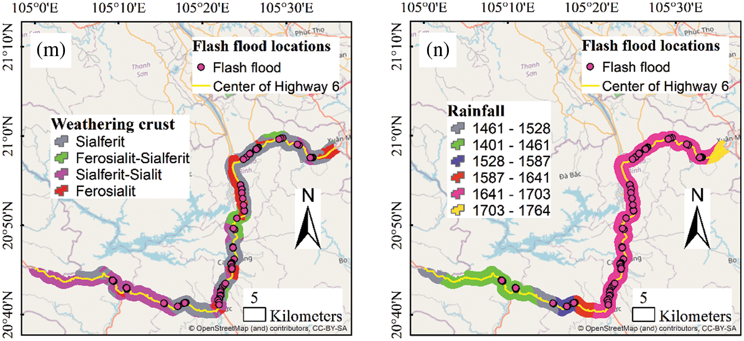
Figure 3: Thematic maps of the study area: (a) elevation, (b) slope, (c) aspect, (d) curvature, (e) TWI, (f) SPI, (g) drainage density, (h) elevation difference, (i) land use, (j) geomorphology, (k) structural zone, (l) lithology, (m) weathering crust, (n) rainfall

4.2.1 Elevation

The elevation has a significant impact on the occurrence of flash floods as it controls the rainfall, vegetation and ice formation [39,40]. At higher elevations, rainfall is generally less in comparison to middle and lower elevations. The elevation map of the area was prepared from DEM (https://search.asf.alaska.edu/) and classified into eleven classes using the natural break method of ArcGIS (Fig. 3a).

4.2.2 Slope

The velocity of surface flow and soil penetration are both affected by the slope angle [41]. At higher slopes, the runoff will be more and the possibility of infiltration is almost negligible. Thus higher slopes in hilly areas have good conditions for devastating flash floods. The slope map was prepared from DEM using ArcGIS tool into 10 classes (Fig. 3b).

4.2.3 Aspect

For flash flood modeling, several topographic parameters such as curvature, and aspect are taken into account [34,39,42]. Aspect plays an important role in the formation of soil, vegetation and moisture on the slope surface thus affect the runoff in the area. The Aspect map was prepared the DEM and classified into nine classes (Fig. 3c).

4.2.4 Curvature

Curvature is one of the important conditioning factor in the occurrence of flood [43,44]. Flat surfaces are most vulnerable for accumulating flood water, whereas curved surfaces are to runoff with velocity. The curvature map of the area was prepared from the DEM and classified into three classes (Fig. 3d).

4.2.5 TWI and SPI

To evaluate topographic management of hydrology procedures, the Topographic-Wetness Index (TWI) and Stream-Power Index (SPI) were frequently utilized [33,45]. SPI describes the flow’s eroding power in the watershed. SPI, an assessment of a flow’s scouring capacity. TWI represent amount flow accumulation in a drainage area and trend of water going down the slope under the effect of gravity. Thematic maps of TWI (Fig. 3e) and SPI (Fig. 4f) were generated from DEM and classified in different classes. TWI can be calculated using the following formula [46]:

TWI=ln⁡(Astan⁡β)(16)

where: AS denotes the typical watershed area (m2/m) and denotes the slope in degrees.

Figure 4: Modeling framework for Flash flood susceptibility prediction

Moore et al. [43] used the following equation to determine SPI:

TWI=As×tan⁡β(17)

4.2.6 Drainage Density

The drainage density plays an important role in flooding of the area [47]. The drainage basin having high drainage density will drain more runoff quickly into the main rain channel, thus helping in flash flood in the event of heavy rains. The overall length of rivers in a watershed represents the length of a hydraulic network [48,49]. The drainage density is computed by splitting the total drainage distance (km) per 1 km2 area. Drainage density map of the area was prepared from the DEM (Fig. 3g).

4.2.7 Elevation Difference

The elevation difference shows the terrain’s relative elevation, which is the height difference between places on the terrain [44,50]. The elevation difference condition states the vertical topography surface variance, which is a key element in flash-flood events because it impacts streamlines, speed, and volume of runoff water. The research area’s elevation difference was calculated using a topographical map at a resolution of 1:50,000 to calculate relative topography elevation (meters) in each uniform grid (per 1 km2) (Fig. 3h).

4.2.8 Land-Use

Land use types influence hydrodynamic procedure attributes such as permeability, evapotranspiration, and runoff creation [51]. Low vegetation areas have more runoff, thus enhancing flash floods. Similarly, areas of impermeable surfaces such as roads building etc. also increase runoff and less infiltration of rain water. A land use map of the study area was obtained from the Department of Agriculture and Rural Development (Fig. 3i).

4.2.9 Geomorphology

Geomorphological features and processes affect the flooding of the area such as river valleys, hill slopes, configuration of drainage basins [42,52]. The geomorphology map of the study area was derived from a 50,000-scale Hoa Binh geomorphic obtained from Vietnam’s Ministry of Natural Resources and Environment. Eleven geomorphic units are represented in this thematic map (Fig. 3j).

4.2.10 Structural Zone

Types of structures affect the natural flow of the water, thus flooding process [31]. In the study area, the NH-route passes three main structural zones: Da River, Fansipan, and Nam Co. (Fig. 3k). This map was derived from the geology map of the area.

4.2.11 Lithology

Lithology is one of the factors which affects the occurrence flash floods [12,31]. Impervious rocks have more runoff in the event of rainfall and thus increasing possibility of flash floods depending on their nature and area distribution. Five lithological classes present the research region (Fig. 3n). The lithological map of the study area was derived from the Hoa Binh lithological map, which was published by the Vietnamese Ministry of Natural Resources and Environment on a scale of 1:50,000.

4.2.12 Weathering Crust

As in the case of geology, the nature and type of weathering crust affect the runoff and infiltration [53,54]. Impervious material forming weathering crust will have more runoff in comparison to previous material. The research site is in a sub-tropical climate that has resulted in a variety of weathering crusts. The weathering crust map was derived from the published map of Hoa Binh province (Scale 1:50,000) of the Vietnamese Ministry of Natural Resources and Environment (Fig. 3m).

4.2.13 Rainfall

Rainfall is one of the main causes of the flooding of the area [4,42]. Heavy rainfall in a short time causes flash floods depending on the topography, drainage and other geo-environmental conditions. The rainfall data of the period from 1998 to 2018 was obtained from five gauge stations in Hoa Binh Province. This study used the inverse distance weighted approach to create a rainfall map (Fig. 3o).

5  Methodology

The methodological framework of the present study included many steps (Fig. 4): (1) Conditioning factor: Initially, flash flood inventory of the area was prepared based on the available record and field survey. A spatial map of flood locations was generated using ArcGIS. Flood conditioning factors were selected based on the local topographic and geo-environmental conditions. (2) Flash flood inventory databased: The collected data of 88 flash flood events were split in 70:30 ratio for training and validation. (3) Modeling process: three models namely DL, CFWNB and AB_CFWNB were generated by using a training dataset. (4) Validation and comparison of the models: Statistical methods were used to evaluate the performance of the models. Results were compared and finally, the best model was selected for the generation of a flash flood susceptibility map. (5) Flash flood susceptibility map: It was assessed in this step by utilizing the parameters generated during the model establishing phase. These metrics were applied to all pixels in the research space’s flash flood area and categorized to estimate susceptible classes using ArcGIS’s naturally breaking classification technique—a convenient approach for defining flood risk susceptibility classes.

6  Results

The importance of the flood conditioning factors was evaluated using feature selection based on IGR, and the results are presented in Table 1. It could be observed that the highest average merit is for elevation factor (0.207), followed by geomorphology (0.184), land-use (0.184), rainfall (0.111), aspect (0.107), drainage density (0.093), elevation difference (0.062), slope (0.048), lithology (0.035), weathering crust (0.029), curvature (0.027), SPI (0.016). In contrast, the two regulatory factors (structural region, TWI) have very small mean values. Therefore, it can be stated that topography and geomorphology are the most important factors in flood modeling in this study.

6.1 Validation and Evaluation of the Models

The standard statistical metrics were used to validate and evaluate the performance of the studied models DL, CFWNB, AB-CFWNB) (Table 2). Results indicated that performance of the DL model is the best in terms of TP (55), TN (55), FP (9), FN (4), PPV (85.938%), NPV (93.220%), SST (93.220%), SPF (85.938%), ACC (89.431%), MAE (0.203), RMSE (0.279) training dataset. Similarly on testing dataset performance of, the DL model is better TP (22), TN (24), FP (3), FN (3), PPV (88.889%), NPV (88.889%), SST (88.899%), SPF (88.899%), ACC (88.462%), MAE (0.234), RMSE (0.352) in comparison to other models (RMSE = 0.424 of CFWNB model and 0.394 of AB_CFWNB).

The DL model on testing data also has the highest K value (0.736) in comparison to CFWNB (0.433) and AB_CFWNB (0.547).

The RMSE analysis on training and testing data sets also indicate that the DL model is having lowest values in both the cases in comparison to other two models (Figs. 5 and 6).

Figure 5: RMSE analysis of the models using the training dataset

Figure 6: RMSE analysis of the models using the validation dataset

The AUC values obtained from the confusion matrix of the model’s results (Fig. 7). The DL model is having highest values (Training: 0.972, Testing: 0.88) on training and testing datasets in comparison to CFWNB (0.829, 0.809), and AB_CFWNB (0.923, 0.85), models. It can be seen that AUC values of all the three studied models are good (AUC > 0.8) but of DL model is the best in the prediction of flood susceptibility.

Figure 7: ROC analysis of the models: (a) training dataset and (b) validation dataset

6.2 Construction of Flash Flood Susceptibility Maps

The flash flood susceptibility values were estimated from the application of three validated models. These values were reclassified into five classes (very low, low, moderate, high, and very high) using the natural break classification method to develop flash flood susceptibility maps for each studied ML model (Fig. 8). The high and extremely high flash flood susceptibility zones along studied sections of the road by three models are 38.1% (DL), 40.8% (CFWNB) and 39.8% (AB_CFWNB) (Fig. 9).

Figure 8: Flash flood susceptibility maps using ML models: (a) DL, (b) CFWNB and (c) AB-CFWNB

Figure 9: Analysis of FR on the susceptibility maps using the models: (a) Frequence ratio, (b) Percentage of class pixels, (c) Percentage of flash flood pixels

The flash flood susceptibility map that the models built were verified by using the Frequency Ratio (FR) as well as the proportion of landslide pixels for every risk class. The FR results from the three models were pretty similar. However, in the high-susceptibility level, the FR-value of the DL model differed significantly from that of the CFWNB and AB-CFWNB models. Besides, the percentage of flood pixels produced by the models did not distinguish considerably. However, the percentage of class pixels differed slightly.

Table 3 shows the results of the density analysis on the flash flood susceptibility maps. The statistical metrics indicate that the performance of the established models is adequate and acceptable. In addition, compared to other models, the map created by DL models is the most reliable, as they gained the greatest values of FR, percent class, and percent LS on the high and very high class.

7  Discussion

Despite the fact that flash floods have become more common in hilly locations, there are few literature reviews on flash flood risk in the transportation industry in Vietnam. In this study, we created new ML models (DL, CFWNB, AB-CFWNB) to produce flash flood susceptibility maps for the NH6 route. The findings of the inquiry have aided the possible implementation of a new machine learning technique to design and map flash-flood risk for a transportation system in Vietnam’s Hoa Binh region. The three models all operate admirably in modeling and mapping the NH6 flash flood susceptibility estimation, in which the DL model was found to be the most accurate. DL is the model commonly used to create landslide susceptibility maps, as well as flood susceptibility maps [6,16,24]. Bui et al. [31] applied a number of models to create flash flood sensitivity maps for Lao Cai Province in Vietnam. At the same time, DL (AUC = 0.96) showed outperformance than MLP-NN (AUC = 0.926) and SVM (AUC = 0.936). It is due to that DL with many hidden layers is capable of exploiting the complicated hidden issue in the GIS dataset. During the deep network training-process, a hierarchical structure is used to build the high-level characteristics that are most adapted for classification tasks. Therefore, the DL model has better flexibility and generalizability. It can be seen that DL appears to be a potential new method for predicting flash floods in flood-prone locations. However, using DL to estimate flash flood susceptibility is still limited in the transport industry. The proposed approach and results can be used to encourage flood hazard mitigation plans along the NH6 in the province of Hoa Binh. The findings could help to improve the use of ML models in hazard identification. Furthermore, the flash-flood risk map can provide better data for flood hazard management, particularly for transportation routes.

It is noteworthy that this study did not consider the dynamics caused by humans such as deforestation, terrain changes, infrastructure improvement, or environmental issues. These factors may bring an effect on natural hydrological processes and, as a result, the frequency of floods, particularly flash floods in residential regions which can cause serious damage to people and property. Another limitation of this study is not enough dynamic assessment of varying situations linked to physiological symptoms, fluid volumes, orientation, erode, deposition, water drainage obstruction, and other factors in flood modeling and their impact on land and flood mitigation. Nevertheless, it is necessary to develop more studies into flash flood estimation, and mapping by employing different combinations of artificial intelligence models in diverse places with high quality geographical information to produce improved flash flood hazard maps.

8  Concluding Remarks

Vietnam is a hilly mountainous country facing flash flood problems affecting normal life besides loss of property, infrastructure and communication disruption in most of the provinces. The flash flood problem in hilly areas is more severe due to the sudden triggering of landslides causing damage to hilly roads, other infrastructures and houses located in the path of a flash flood on the slopes and in the valleys. Therefore, in the hilly terrain, accurate prediction of flash flood susceptible areas will help properly plan and maintain roads and other infrastructure facilities. In the present study, three novel ML models were applied to develop flash flood susceptibility maps along part of the NH-6, a hilly road section passing through Hoa Binh province of Vietnam. The results revealed that all the models performed well (AUC > 0.80) in predicting flash flood susceptibility zones, but the performance of the DL model is the best (AUC: 0.972, RMSE: 0.352). Therefore, it can be concluded that the DL model can be used for the accurate prediction of flash flood susceptibility zones not only in the study area but also in other hilly areas. The limitation of the study is that we could not use time series rainfall data in the models. In future studies, we will refine the models’ performance with more input parameters in the present study and new ensemble DL models.

Funding Statement: This research is funded by Vietnam National Foundation for Science and Technology Development (NAFOSTED) under Grant No. 105.08-2019.03.

Conflicts of Interest: The authors declare that they have no conflicts of interest to report regarding the present study.

References

 1.  Cao, C., Xu, P., Wang, Y., Chen, J., Zheng, L. et al. (2016). Flash flood hazard susceptibility mapping using frequency ratio and statistical index methods in coalmine subsidence areas. Sustainability, 8(9), 948. DOI 10.3390/su8090948. [Google Scholar] [CrossRef]

 2.  Bui, D. T., Ngo, P. T. T., Pham, T. D., Jaafari, A., Minh, N. Q. et al. (2019). A novel hybrid approach based on a swarm intelligence optimized extreme learning machine for flash flood susceptibility mapping. Catena, 179, 184–196. DOI 10.1016/j.catena.2019.04.009. [Google Scholar] [CrossRef]

 3.  Pham, B. T., Luu, C., van Phong, T., Trinh, P. T., Shirzadi, A. et al. (2021). Can deep learning algorithms outperform benchmark machine learning algorithms in flood susceptibility modeling? Journal of Hydrology, 592, 125615. DOI 10.1016/j.jhydrol.2020.125615. [Google Scholar] [CrossRef]

 4.  Bubeck, P., Botzen, W. J. W., Aerts, J. C. (2012). A review of risk perceptions and other factors that influence flood mitigation behavior. Risk Analysis, 32(9), 1481–1495. DOI 10.1111/j.1539-6924.2011.01783.x. [Google Scholar] [CrossRef]

 5.  Choubin, B., Moradi, E., Golshan, M., Adamowski, J., Sajedi-Hosseini, F. et al. (2019). An ensemble prediction of flood susceptibility using multivariate discriminant analysis, classification and regression trees, and support vector machines. Science of the Total Environment, 651, 2087–2096. DOI 10.1016/j.scitotenv.2018.10.064. [Google Scholar] [CrossRef]

 6.  Costache, R., Arabameri, A., Blaschke, T., Pham, Q. B., Pham, B. T. et al. (2021). Flash-flood potential mapping using deep learning, alternating decision trees and data provided by remote sensing sensors. Sensors, 21(1), 280. DOI 10.3390/s21010280. [Google Scholar] [CrossRef]

 7.  Hosseini, F. S., Choubin, B., Mosavi, A., Nabipour, N., Shamshirband, S. et al. (2020). Flash-flood hazard assessment using ensembles and Bayesian-based machine learning models: Application of the simulated annealing feature selection method. Science of the Total Environment, 711, 135161. DOI 10.1016/j.scitotenv.2019.135161. [Google Scholar] [CrossRef]

 8.  Bui, D. T., Tsangaratos, P., Ngo, P. T. T., Pham, T. D., Pham, B. T. (2019). Flash flood susceptibility modeling using an optimized fuzzy rule based feature selection technique and tree based ensemble methods. Science of the Total Environment, 668, 1038–1054. DOI 10.1016/j.scitotenv.2019.02.422. [Google Scholar] [CrossRef]

 9.  Ha Thi, H. (2018). Application of remote sensing and GIS for flood vulnerability and mitigation: A case study of flood affected Highway 6, Hoa Binh Province. International Symposium on Geoinformatics for Spatial Infrastructure Development in Earth and Allied Sciences 2018. https://gisws.media.osaka-cu.ac.jp/gisideas18/viewpaper.php?id=689. [Google Scholar]

10. Janizadeh, S., Avand, M., Jaafari, A., Phong, T. V., Bayat, M. et al. (2019). Prediction success of machine learning methods for flash flood susceptibility mapping in the Tafresh watershed, Iran. Sustainability, 11(19), 5426. DOI 10.3390/su11195426. [Google Scholar] [CrossRef]

11. Pham, B. T., Phong, T. V., Nguyen, H. D., Qi, C., Al-Ansari, N. et al. (2020). A comparative study of kernel logistic regression, radial basis function classifier, multinomial Naïve Bayes, and logistic model tree for flash flood susceptibility mapping. Water, 12(1), 239. DOI 10.3390/w12010239. [Google Scholar] [CrossRef]

12. Ha, H., Luu, C., Bui, Q. D., Pham, D. H., Hoang, T. et al. (2021). Flash flood susceptibility prediction mapping for a road network using hybrid machine learning models. Natural Hazards, 109(1), 1247–1270. DOI 10.1007/s11069-021-04877-5. [Google Scholar] [CrossRef]

13. Jun, C. L., Mohamed, Z. S., Peik, A. L., Razali, S. F., Sharil, S. (2016). Flood forecasting model using empirical method for a small catchment area. Journal of Engineering Science and Technology, 11(5), 666–672. [Google Scholar]

14. Lee, B. J., Kim, S. (2019). Gridded flash flood risk index coupling statistical approaches and TOPLATS land surface model for mountainous areas. Water, 11(3), 504. DOI 10.3390/w11030504. [Google Scholar] [CrossRef]

15. Hapuarachchi, H., Wang, Q., Pagano, T. (2011). A review of advances in flash flood forecasting. Hydrological Processes, 25(18), 2771–2784. DOI 10.1002/hyp.8040. [Google Scholar] [CrossRef]

16. Panahi, M., Jaafari, A., Shirzadi, A., Shahabi, H., Rahmati, O. et al. (2021). Deep learning neural networks for spatially explicit prediction of flash flood probability. Geoscience Frontiers, 12(3), 101076. DOI 10.1016/j.gsf.2020.09.007. [Google Scholar] [CrossRef]

17. Nielsen, M. A. (2015). Neural networks and deep learning, vol. 25. San Francisco, CA, USA: Determination Press. [Google Scholar]

18. Schmidhuber, J. (2015). Deep learning in neural networks: An overview. Neural Networks, 6185–117. DOI 10.1016/j.neunet.2014.09.003. [Google Scholar] [CrossRef]

19. Goodfellow, I., Bengio, Y., Courville, A. (2016). Deep learning. Cambridge, Massachusetts, USA: MIT Press. [Google Scholar]

20. Kim, P. (2017). MATLAB deep learning. Apress Berkeley, CA. DOI 10.1007/978-1-4842-2845-6. [Google Scholar] [CrossRef]

21. Petersen, P., Voigtlaender, F. (2018). Optimal approximation of piecewise smooth functions using deep ReLU neural networks. Neural Networks, 108, 296–330. DOI 10.1016/j.neunet.2018.08.019. [Google Scholar] [CrossRef]

22. Huang, Z., Li, J., Weng, C., Lee, C. H. (2014). Beyond cross-entropy: Towards better frame-level objective functions for deep neural network training in automatic speech recognition. Fifteenth Annual Conference of the International Speech Communication Association, Singapore. [Google Scholar]

23. Jiang, L., Zhang, L., Li, C., Wu, J. (2018). A Correlation-based feature weighting filter for Naive Bayes. IEEE Transactions on Knowledge and Data Engineering, 31(2), 201–213. DOI 10.1109/TKDE.69. [Google Scholar] [CrossRef]

24. Freund, Y., Schapire, R. E. (1997). A decision-theoretic generalization of on-line learning and an application to boosting. Journal of Computer and System Sciences, 55(1), 119–139. DOI 10.1006/jcss.1997.1504. [Google Scholar] [CrossRef]

25. Pham, B. T., Tien Bui, D., Indra, P., Dholakia, M. (2015). Landslide susceptibility assessment at a part of uttarakhand himalaya, India using GIS–based statistical approach of frequency ratio method. International Journal of Engineering Research & Technology, 4(11), 338–344. [Google Scholar]

26. Sun, J., Jia, M. Y., Li, H. (2011). AdaBoost ensemble for financial distress prediction: An empirical comparison with data from Chinese listed companies. Expert Systems with Applications, 38(8), 9305–9312. DOI 10.1016/j.eswa.2011.01.042. [Google Scholar] [CrossRef]

27. Tien Bui, D., Ho, T. C., Pradhan, B., Pham, B. T., Nhu, V. H. et al. (2016). GIS-based modeling of rainfall-induced landslides using data mining-based functional trees classifier with AdaBoost, Bagging, and MultiBoost ensemble frameworks. Environmental Earth Sciences, 75(14), 1–22. [Google Scholar]

28. Pham, B. T., Bui, D. T., Prakash, I., Dholakia, M. (2017). Hybrid integration of multilayer perceptron neural networks and machine learning ensembles for landslide susceptibility assessment at Himalayan area (India) using GIS. Catena, 149, 52–63. DOI 10.1016/j.catena.2016.09.007. [Google Scholar] [CrossRef]

29. Hoang, N. D., Bui, D. T. (2018). Predicting earthquake-induced soil liquefaction based on a hybridization of kernel fisher discriminant analysis and a least squares support vector machine: A multi-dataset study. Bulletin of Engineering Geology and the Environment, 77(1), 191–204. DOI 10.1007/s10064-016-0924-0. [Google Scholar] [CrossRef]

30. Nhu, V. H., Mohammadi, A., Shahabi, H., Ahmad, B. B., Al-Ansari, N. et al. (2020). Landslide detection and susceptibility modeling on cameron highlands (MalaysiaA comparison between random forest, logistic regression and logistic model tree algorithms. Forests, 11(8), 830. DOI 10.3390/f11080830. [Google Scholar] [CrossRef]

31. Bui, D. T., Hoang, N. D., Martínez-Álvarez, F., Ngo, P. T. T., Hoa, P. V. et al. (2020). A novel deep learning neural network approach for predicting flash flood susceptibility: A case study at a high frequency tropical storm area. Science of the Total Environment, 701, 134413. DOI 10.1016/j.scitotenv.2019.134413. [Google Scholar] [CrossRef]

32. van Dao, D., Jaafari, A., Bayat, M., Mafi-Gholami, D., Qi, C. et al. (2020). A spatially explicit deep learning neural network model for the prediction of landslide susceptibility. Catena, 188, 104451. DOI 10.1016/j.catena.2019.104451. [Google Scholar] [CrossRef]

33. Termeh, S. V. R., Kornejady, A., Pourghasemi, H. R., Keesstra, S. (2018). Flood susceptibility mapping using novel ensembles of adaptive neuro fuzzy inference system and metaheuristic algorithms. Science of the Total Environment, 615, 438–451. DOI 10.1016/j.scitotenv.2017.09.262. [Google Scholar] [CrossRef]

34. Versini, P. A., Gaume, E., Andrieu, H. (2010). Assessment of the susceptibility of roads to flooding based on geographical information–test in a flash flood prone area (the Gard region, France). Natural Hazards and Earth System Sciences, 10(4), 793–803. DOI 10.5194/nhess-10-793-2010. [Google Scholar] [CrossRef]

35. Youssef, A. M., Pradhan, B., Hassan, A. M. (2011). Flash flood risk estimation along the St. Katherine road, Southern Sinai, Egypt using GIS based morphometry and satellite imagery. Environmental Earth Sciences, 62(3), 611–623. DOI 10.1007/s12665-010-0551-1. [Google Scholar] [CrossRef]

36. Reyes, J., Morales-Esteban, A., Martínez-Álvarez, F. (2013). Neural networks to predict earthquakes in Chile. Applied Soft Computing, 13(2), 1314–1328. DOI 10.1016/j.asoc.2012.10.014. [Google Scholar] [CrossRef]

37. Quinlan, J. R. (1993). C4.5: Programming for machine learning. Morgan Kauffmann, 38(48), 49. [Google Scholar]

38. Wang, X., Borgelt, C. (2004). Information measures in fuzzy decision trees. 2004 IEEE International Conference on Fuzzy Systems (IEEE Cat. No. 04CH37542), vol. 1, pp. 85–90. Budapest, Hungary, IEEE. [Google Scholar]

39. Arabameri, A., Saha, S., Chen, W., Roy, J., Pradhan, B. et al. (2020). Flash flood susceptibility modelling using functional tree and hybrid ensemble techniques. Journal of Hydrology, 587, 125007. DOI 10.1016/j.jhydrol.2020.125007. [Google Scholar] [CrossRef]

40. Tien Bui, D., Hoang, N. D. (2017). A Bayesian framework based on a Gaussian mixture model and radial-basis-function fisher discriminant analysis (BayGmmKda V1.1) for spatial prediction of floods. Geoscientific Model Development, 10(9), 3391–3409. DOI 10.5194/gmd-10-3391-2017. [Google Scholar] [CrossRef]

41. Chen, W., Li, Y., Xue, W., Shahabi, H., Li, S. et al. (2020). Modeling flood susceptibility using data-driven approaches of Naïve Bayes tree, alternating decision tree, and random forest methods. Science of the Total Environment, 701, 134979. DOI 10.1016/j.scitotenv.2019.134979. [Google Scholar] [CrossRef]

42. Abuzied, S., Yuan, M., Ibrahim, S., Kaiser, M., Saleem, T. (2016). Geo-spatial risk assessment of flash floods in Nuweiba area, Egypt. Journal of Arid Environments, 133, 54–72. DOI 10.1016/j.jaridenv.2016.06.004. [Google Scholar] [CrossRef]

43. Moore, I. D., Grayson, R., Ladson, A. (1991). Digital terrain modelling: A review of hydrological, geomorphological, and biological applications. Hydrological Processes, 5(1), 3–30. DOI 10.1002/(ISSN)1099-1085. [Google Scholar] [CrossRef]

44. Wilford, D., Sakals, M., Innes, J., Sidle, R. C., Bergerud, W. (2004). Recognition of debris flow, debris flood and flood hazard through watershed morphometrics. Landslides, 1(1), 61–66. DOI 10.1007/s10346-003-0002-0. [Google Scholar] [CrossRef]

45. Yariyan, P., Janizadeh, S., Van Phong, T., Nguyen, H. D., Costache, R. et al. (2020). Improvement of best first decision trees using bagging and dagging ensembles for flood probability mapping. Water Resources Management, 34(9), 3037–3053. DOI 10.1007/s11269-020-02603-7. [Google Scholar] [CrossRef]

46. Beven, K. J., Kirkby, M. J. (1979). A physically based, variable contributing area model of basin hydrology/Un modèle à base physique de zone d’appel variable de l’hydrologie du bassin versant. Hydrological Sciences Journal, 24(1), 43–69. DOI 10.1080/02626667909491834. [Google Scholar] [CrossRef]

47. Naulin, J. P., Payrastre, O., Gaume, E. (2013). Spatially distributed flood forecasting in flash flood prone areas: Application to road network supervision in Southern France. Journal of Hydrology, 486, 88–99. DOI 10.1016/j.jhydrol.2013.01.044. [Google Scholar] [CrossRef]

48. Bhatawdekar, R. M., Singh, T. N., Tonnizam Mohamad, E., Armaghani, D. J., Binti Abang Hasbollah, D. Z. (2021). River sand mining vis a vis manufactured sand for sustainability. Proceedings of the International Conference on Innovations for Sustainable and Responsible Mining, pp. 143–169. Hanoi, Vietnam, Springer. [Google Scholar]

49. Kumar, B. S., Zainuddin, M. F. B., Soon, D. C. H., Bhatawdekar, R. M. (2022). Learning lessons from river sand mining practices in India and Malaysia for sustainability. Risk, Reliability and Sustainable Remediation in the Field of Civil and Environmental Engineering, vol. 2022, pp. 315–331. India, Elsevier. [Google Scholar]

50. Pradhan, B. (2013). A comparative study on the predictive ability of the decision tree, support vector machine and neuro-fuzzy models in landslide susceptibility mapping using GIS. Computers & Geosciences, 51, 350–365. DOI 10.1016/j.cageo.2012.08.023. [Google Scholar] [CrossRef]

51. Khosravi, K., Pham, B. T., Chapi, K., Shirzadi, A., Shahabi, H. et al. (2018). A comparative assessment of decision trees algorithms for flash flood susceptibility modeling at Haraz watershed, Northern Iran. Science of the Total Environment, 627, 744–755. DOI 10.1016/j.scitotenv.2018.01.266. [Google Scholar] [CrossRef]

52. Costache, R., Bui, D. T. (2020). Identification of areas prone to flash-flood phenomena using multiple-criteria decision-making, bivariate statistics, machine learning and their ensembles. Science of the Total Environment, 712, 136492. DOI 10.1016/j.scitotenv.2019.136492. [Google Scholar] [CrossRef]

53. Casale, R., Margottini, C. (1999). Floods and landslides: Integrated risk assessment: Integrated risk assessment; with 30 tables. Berlin, Germany: Springer Science & Business Media. [Google Scholar]

54. González-Arqueros, M. L., Mendoza, M. E., Bocco, G., Castillo, B. S. (2018). Flood susceptibility in rural settlements in remote zones: The case of a mountainous basin in the Sierra-Costa region of Michoacán, Mexico. Journal of Environmental Management, 223, 685–693. DOI 10.1016/j.jenvman.2018.06.075. [Google Scholar] [CrossRef]