A Smooth Bidirectional Evolutionary Structural Optimization of Vibrational Structures for Natural Frequency and Dynamic Compliance

1  Introduction

Topology optimization has been widely applied to various engineering field such as submerged, aeronautics and automobile structures, due to significant improvement of structural performance [1–3]. In the past four decades, many gradient-or heuristic-based optimization methods have been developed, including Homogenization, Density, Level Set, Evolutionary Structural Optimization (ESO) and a Bidirectional Version of ESO (BESO) [4].

ESO and BESO gradually remove the unnecessary region from the structure using binary methods, such that the resulting structure evolves to clear (0/1) designs along the optimal direction. However, undue removal of elements can induce an inefficient local optimum and even failure to convergence [5]. To resolve the issue, Almeida et al. [6] firstly proposed a variant of the ESO procedure called Smooth ESO (SESO), which gradually removed an unnecessary element for the structure by reducing the values of the constitutive matrix. SESO is superior to the classical ESO method, which is demonstrated in those works [7–10]. The benchmark examples reveal that the procedure known as progressive “soft-kill” produces a clean and smooth boundary and dwindles the checkerboard formation in the resulting optimal structure. Under dynamic loading, a structural response such as displacements and internal stresses, are time-varying. Thus, dynamic topology optimization is still confronted with great challenges such as prohibitively high computational cost and complex sensitivity derivation [4,11]. Although the SESO technique can solve topology optimization problems of 2D elastic structures in a simple and efficient way, it has not been extended to the topology optimization under dynamic loading due to above mentioned unresolved challenges.

Published dynamic topology optimization researches mainly focus on three main problems including eigenfrequency optimization [12–15], dynamic response optimization under steady-state [16–19] and transient [20–24] excitations. In eigenfrequency optimization, researchers provide an efficient way such as maximization of the specified eigenfrequencies or the bandwidth to avoid structural resonance. Although certain dynamic characteristics like natural frequency can be tailored to the designer’s choice, these eigenfrequency optimizations do not directly dominate the structural response under dynamic loading. To optimize the dynamic response under steady-state forced vibration, a frequently adopted method is to discretize the frequency range into substantial frequency points and then minimize the dynamic compliance of structures subjected to external harmonic excitation [16–18]. One defect of the dynamic compliance problem is a large computational burden due to the harmonic analysis at each discretized frequency in the loading frequency bands. To efficiently solve the dynamic response in the frequency domain, the modal decomposition method is used to remarkably eliminate the computational demand for continuum structures [19]. To tackle the topology optimization problems of dynamic response in the time domain, two approaches have been developed including time-integration method scheme like Newmark-β [20,21] and the equivalent static load (ESL) method [22–24] so far. Generally speaking, the former has some obstacles in engineering application due to a quite time-consuming modelling, complex and challenging sensitivity analysis. The latter transforms the dynamic topology optimization problem into a static one with multiple loading cases, which has been mathematically justified to avoid falling into a local optimum solution [25]. Therefore, the ESL method is used to perform the topology optimization of transient response in the present work.

The SESO technique provides a mathematical programming tool for engineers and architects who seek efficient distribution of material in structural boundary value problems during the conceptual design stage of a project. This paper proposes a bidirectional version of SESO (SBESO), which is potentialized to solve the topological optimization of vibrating continuum structures for natural frequencies and dynamic compliance under the transient load. The remainder of the paper is organized as follows: Section 2 disposes of the formulation of the dynamic problem using SBESO. Section 3 formulates the eigenfrequency optimization problem. Section 4 formulates the dynamic compliance optimization problem using the ESL method. The numerical results are presented from the proposed SBESO method in eigenfrequency and dynamic compliance optimization. Finally, concluding remarks are made in Section 5.

2  Smooth Bidirectional Evolutionary Structural Optimization (SBESO)

Based on the evolutionary structure optimization method, the mathematical model of structural dynamics topology optimization is expressed as follows:

Minimize f(x)s.t.V∗−∑i=1NVixi=0M(x)u¨(t)+K(x)u(t)=F(t)xi=0or1(i=1,…,N)(1)

where f(x) is the objective function, x=[xi]N×1 is the design variable as vectors of element densities (where xi=0 denotes a void element and xi=1 denotes a solid one), V∗ is the specified volume fraction and Vi are the volume of element. M(x) and K(x) are the global mass and stiffness matrix. u¨(t) and u(t) are the corresponding acceleration and displacement responses of a structure under the transient load F(t).

For the traditional BESO method, all the elements are sorted in ascending order in terms of calculated sensitivity numbers of the objective function to the design variables. Then the elements with high sensitivity numbers are added to the design domain while those with low sensitivity numbers are removed from the design domain. This scheme is known as hard kill and can be illuminated as the following the evolutionary criteria:

Di(α¯ji)={1j∈Γi{α¯ji≥α¯addi}0j∈Γ¯i{α¯ji≤α¯deli}(2)

where Di(α¯ji) is the evolutionary criterion function, and α¯ji is the filtered sensitivity numbers of the element j at the i-th iteration. α¯addi and α¯deli are the threshold sensitivity numbers for removal and addition of elements, respectively. Γi={α¯ji≥α¯addi} is the set of elements added to the current design domain while Γ¯i={α¯ji≤α¯deli} is those deleted from the current design domain.

However, simple removal of the elements in the iteration based on Eq. (2b), can always cause a premature withdrawal of elements, which should not be deleted. It is often seen that a certain element was wrongly removed to be subjected to Eq. (2b). The obtained solution is non-optimal and even suffers from a numerical instability called “chessboard” due to the ill-conditioning model of the stiffness matrix. To address this issue, the bidirectional version of SESO, SBESO is proposed to organize the elements satisfying Eq. (2) so that q% of these elements are deleted and the remaining (1 − q%) is returned to the current design domain. This return is followed by a regular function that weights the mass and stiffness matrixes of elements in the domain Γ¯i with a higher sensitivity number. This methodology presents proper condition numbers for solving the updated system equation in the next iteration on account that returned elements are significant to the structure.

As shown in Fig. 1, the soft kill scheme employed in the SBESO technique can be illustrated as:

Dis(α¯ji)={1j∈Γi{α¯ji≥α¯addi}η(α¯ji)j∈ΓGS{α¯LSi≤α¯ji≤α¯deli}0j∈ΓLS{α¯ji<α¯LSi}(3)

where 0≤η(α¯ji)≤1 is a weighted function that regulates the mass and stiffness matrix of each element within the domain ΓGS. η(α¯ji) can generally be taken as a linear function η(α¯ji)=ξα¯ji+ζ, a sine function η(α¯ji)=sin⁡(ξα¯ji), and a constant function η(α¯ji)=η0. The former two functions are continuous and differential in the domain Γ¯i. The latter function is discontinuous, where the parameter η0=0 represents the degeneration of SBESO to the classic BESO.

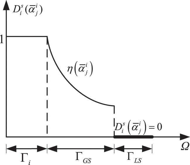
Figure 1: Evolutionary optimization criteria for the SBESO method

For the SBESO method, according to Eq. (3), the mass and stiffness matrices of an element are expressed as:

Mji=Dis(α¯ji)Mji−1(4)

Kji=Dis(α¯ji)Kji−1(5)

where Mji and Kji are the mass and stiffness matrices of the element at the current iteration. Mji−1 and Kji−1 are the mass and stiffness matrices of that at the previous iteration. Particularly, if the element removal rate q% reaches 100%, the SBESO method degenerates into the traditional BESO method, and thus the Eqs. (4) and (5) are rewritten as:

Mji=Di(α¯ji)Mj0(6)

Kji=Di(α¯ji)Kj0(7)

where Mj0 and Kj0 are the initial mass and stiffness matrices of the element, respectively.

Based on classical FE theory, the structural dynamics governing equation is written as:

Mu¨(t)+Ku(t)=F(t)(8)

According to Eqs. (6) and (7), the global mass and stiffness matrices of Eq. (8) in the current design domain of the structure are updated as:

M=∑j∈ΓiMji−1+∑j∈ΓGSη(α¯ji)Mji−1(9)

K=∑j∈ΓiKji−1+∑j∈ΓGSη(α¯ji)Kji−1(10)

When the volume constraint is satisfied and the minimum of the objective function is convergent, the optimal process terminates and the final solution is achieved. The convergence criterion adopted by Huang et al. [12] is used in this study, and can be expressed as:

error=|∑i=1N′fk−i+1−∑i=1N′fk−N′−i+1|/∑i=1N′fk−i+1≤ε1(11)

where error is the relative error of the objective function, and ε1 is the defined convergence tolerance, N′ is an integer which is selected as 5 for all examples using the SBESO method in this study.

As a such, in the light of the above discussion, the flowchart of dynamic topology optimization by SBESO is depicted in Fig. 2 and the topology optimization procedure is given as follows:

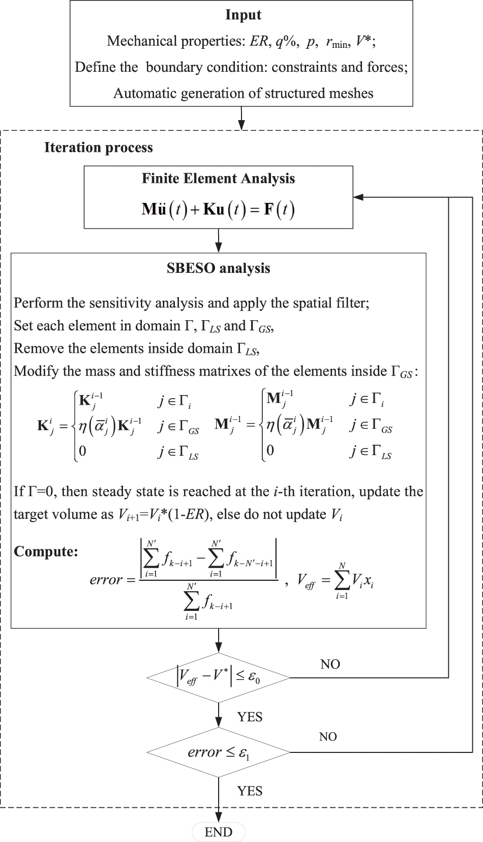
Figure 2: Dynamic topology optimization flowchart by SBESO

Step. 1 Set the algorithm parameters: evolution rate ER, element removal rate q%, target volume V∗, filter radius of sensitivity rmin and penalty factor p, and discretize the initial design domain with a refined finite element mesh;

Step. 2 Perform the dynamic FE analysis on the current design domain to obtain the elemental and nodal sensitivity numbers, and apply spatial filter scheme to smooth the sensitivity numbers of all elements;

Step. 3 Determine the target volume at the next iteration according to the evolutionary rate;

Step. 4 Divide the elements satisfying Eq. (2b) into the two sets: q% of these elements with high sensitivity numbers for removal and (1 − q%) with high sensitivity numbers for return to the structure, setting each element in domains Γi, ΓGS or ΓLS;

Step. 5 Add the elements that are within the domain Γi, delete the elements within the domain ΓLS, and regulate the mass and stiffness matrices of the elements within the domain ΓGS using the specified weighted function;

Step. 6 If Γ¯=0, then the steady state arrives at the i-th iteration and update the target volume as Vi+1=Vi(1−ER), else do not update Vi.

Step. 7 Repeat Steps 2–6 until the objective volume (V*) is achieved and the convergence criteria is met.

3  Frequency Optimization

3.1 Problem Statement

When the dynamic response of a structure is dominated by several vibration modes, one method to diminish excessive vibration is to perform the eigenfrequency topology optimization to prevent the fundamental frequencies from approaching the working frequency. Therefore, the natural frequency corresponding to the vibration mode must be increased to avoid the structural resonance.

For undamped vibration systems, the natural frequency ωl and the eigenvector φl of mode l are interrelated to each other by Rayleigh quotient expressed as:

ωl2=φlTKφl/φlTMφl(12)

Here, the topology optimization problem to maximize the l-th eigenfrequency of a vibrating structure can be stated as:

Maximize f(x)=ωls.t.V∗−∑i=1NVixi=0ωl2=φlTK(x)φl/φlTM(x)φlxi=0or1(i=1,…,N)(13)

3.2 Sensitivity Analysis

Substituting Eqs. (9) and (10) into Eq. (12), the Rayleigh quotient is rewritten by:

[ωli]2=φlT[∑j∈ΓiKji−1+∑j∈ΓGSη(α¯ji)Kji−1]φl/φlT[∑j∈ΓiMji−1+∑j∈ΓGSη(α¯ji)Mji−1]φl(14)

According to Eq. (14), considering the material interpolation scheme, the sensitivity of the objective function can be expressed by:

αji={12ωliφlT(Kji−[ωli]2pMji)φlxj=1−ωli2pφlTMjiφlxj=0(15)

The above equation seems that the sensitivity number is dependent on the penalty factor, normally p≥3, employed in the SIMP model for topology optimization problems. Thus, p = 3 is adopted in this paper.

3.3 Numerical Example

As shown in Fig. 3, we intend to maximize the first natural frequency of a beam-like structure for a specified material volume fraction V* = 50%. The beam with dimensions 240 mm × 30 mm is discretized into 240 × 30 4-node bilinear plane stress elements with same size. The material is modeled as linear elasticity with Young’s modulus of E = 10 GPa, Poisson’s ratio μ = 0.3, and mass density ρ = 1 × 103 Kg/m3. The weight function is selected as a linear function. The SBESO algorithm parameters are as follows: element removal rate q% = 40%–100%, convergence tolerance ɛ0 = ɛ1 = 0.001, sensitivity filtering radius rmin = 5 mm, evolutionary rate ER = 2%.

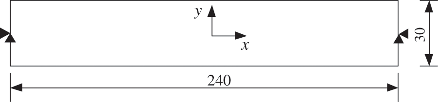
Figure 3: Initial design domain of a beam simply supported at both ends

Fig. 4 illustrates final topologies as well as evolution history of the first natural frequency using SBESO technique with various element removal rate. It is observed that the decreasing element removal rate results in an increasingly smooth evolution history. Particularly, the optimal topology tends to be identical as the element removal rate gradually decreases. For the classic BESO method corresponding to q% = 100%, the strong discontinuity during the iteration of the first natural frequency occurs due to excessive deletion of elements in the structure topology, as shown in Fig. 4a. In contrast, the SBESO method provides a relatively smooth evolution history of first natural frequency, as shown in Figs. 4b–4d. Moreover, the SBESO method produces a relatively stable convergent process compared with the classic BESO method. The optimal natural frequency obtained from the SBESO method is higher than that from classic BESO method. It is notable that the evolutionary history corresponding to q% = 40% smoothly iterates without any jump, which occurs in cases of q% = 70% and 60%, although they share almost the same optimal topology, as shown in Figs. 4b–4d. It attributes to a high element removal rate, which can generate an instable optimal process due to improper removal of efficient elements in a single iteration. As such, it demonstrates that the optimal solution with q% = 40% is more robust when compared with those obtained from other element removal rates. However, low element removal rate can produce expensive computation especially for dynamic optimization. From above analysis, the element removal rate behaves as the step size in mathematical programming which a strong influence on optimization process.

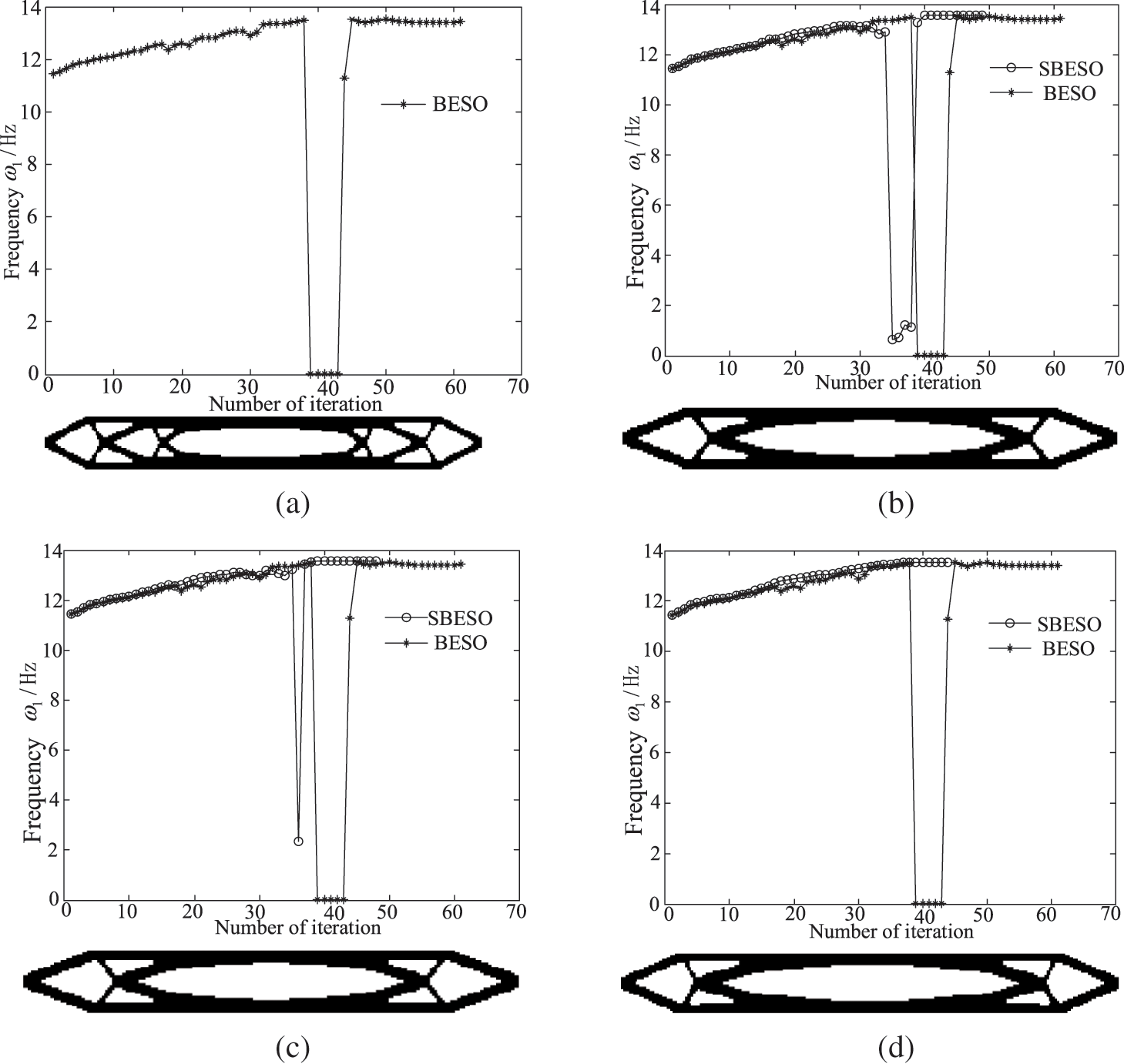
Figure 4: Effect of the deletion rate q% on the optimization topology and convergence process (a) q% = 100% (BESO) (b) q% = 70% (c) q% = 60% (d) q% = 40%

Fig. 5 depicts the effect of various weighted functions on optimal topology and convergence process with q% = 40%. Like the linear weighted function, the sinusoidal form can achieve the relatively smooth iterative process, compared with the constant weighted function. These two continuous weighted functions produce the identical final topology whereas they are different from the constant weighted function. Despite this, the SBESO using the constant weighted function produces the slightly high optimal first natural frequency with a similar final topology to the BESO method. Either the linear or the sinusoidal weighted function monotonously represents the contribution of returned (1 − q%) of the elements, which are removed in the BESO procedure, to the element mass and stiffness matrixes by ranking their sensitivity numbers according to Eqs. (3)–(5). However, the constant weighted function has the returned (1 − q%) of the elements to play the same role on the element mass and stiffness matrixes. Consequently, the linear or the sinusoidal weighted functions share the common optimal topology while the constant weighted function generates the similar optimal topology to that from the BESO method.

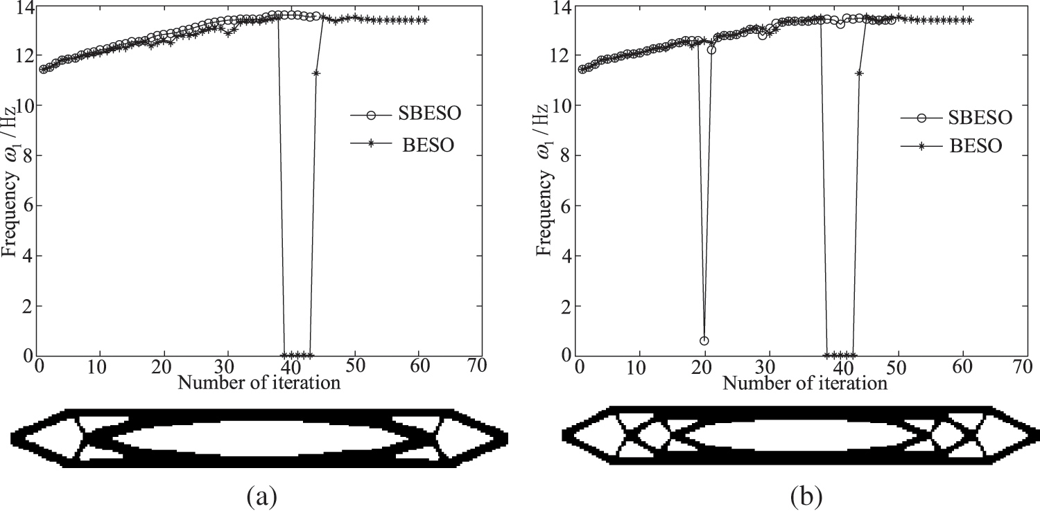
Figure 5: Effect of various weighted functions on optimal topology and convergence process with q% = 40% (a) Sinusoidal function (b) Constant function

4  Dynamic Compliance Optimization

4.1 Problem Statement

The topology optimization of dynamic compliance for a structure under transient loading is formulated with limited available material. The average dynamic compliance over the entire time is minimized to maximize the stiffness of the structure and can be mathematically expressed as:

Minimize C(x)=1m∑r=1m12FT(tr)u(tr)s.t.V∗−∑i=1NVixi=0M(x)u¨(tr)+K(x)u(tr)=F(tr)xi=0or1(i=1,…,N)(16)

where F(tr) is the external force vector at the r-th time step, and m is the number of time steps. u¨(tr) and u(tr) are the acceleration and displacement vectors at the r-th time step, respectively.

To avoid the complex dynamic sensitivity analysis in the time domain, the ESL method is used for the dynamic topology optimization problem in this study. The HHT-α scheme is also employed to solve the structural dynamics problem.

4.2 HHT-α Method

The HHT-α method generalizes from the Newmark-β method, which is employed to calculate the structural dynamic response under the transient loading. The HHT-α method alters the momentum equation by a parameter α describing a numerical delay between stiffness and external force vector, expressed as:

M(x)u¨(tr)+(1−α)K(x)u(tr)+αK(x)u(tr−1)=(1−α)F(tr)+αF(tr−1),r=1,…,m(17)

u(tr)=u(tr−1)+Δtu˙(tr−1)+Δt2[(1/2−β)u¨(tr−1)+βu¨(tr)](18)

u˙(tr)=u˙(tr−1)+Δt[(1−γ)u¨(tr−1)+γu¨(tr)](19)

The HHT-α method is adopted along with the finite difference algorithm of the Newmark-β, such that it degenerates into the Newmark-β when α = 0.

To guarantee that the Newmark-β method is provided with at least second-order accuracy and unconditional stability, α, β, and γ are subject to the following conditions:

0≤α≤1/3,β=(1+α)2/4,γ=(1+2α)/2(20)

By substitution of Eq. (17) into Eq. (16b), the discrete momentum equation is acquired as:

M1(x)u¨(tr)+M0(x)u¨(tr−1)+K(x)u(tr−1)−(1−α)F(tr)−αF(tr−1)=0(21)

where

M1(x)=M(x)+(1−α)βΔt2K(x)M0(x)=(1−α)(1/2−β)Δt2K(x)(22)

To obtain the dynamic response at every time step, we calculate u¨(tr) from Eq. (21) and then update u(tr) and u˙(tr) using Eqs. (18) and (19). For initial time step, we compute u¨(t0) as u¨(t0)=M(x)−1(F(t0)−K(x)u(t0)) from the specified u(t0) and u˙(t0).

4.3 ELS-Based Computation Flow of Optimization

Equivalent static load refers to the static load that produces the identical displacement field to that of dynamic analysis. Because the dynamic displacement is computed at every time step, the ESL set is obtained over the entire time. Total ESL sets are employed as multiple loading to solve the corresponding static optimization problem, which shares the same optimal solution as original dynamic optimization problem.

The ESL vector feq(tr), can be obtained using the displacement field from Eq. (18) as follows:

feq(tr)=K(x)u(tr)(r=1,…,m)(23)

Once the ESL vector is computed, it is employed in the equilibrium equation as the r-th external loading for static optimization expressed as:

K(x)us(tr)=feq(tr)(r=1,…,m)(24)

where us(tr) denotes the static displacement response to the r-th external loading. The subscript s represents static condition.

The ESL optimization consists of an analysis domain and a design domain, as shown in Fig. 6. The analysis domain performs structural dynamic analysis to obtain the displacement field at each time step, which is used to calculate ESL sets. Then the ESL sets are transferred to the design domain for the linear static optimization with multiple loading conditions. The design variables are updated and returned to the analysis domain to recalculate the displacement field.

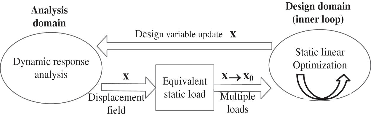
Figure 6: Iterative process of the equivalent static load method

In the design domain for static response optimization, an objective function is defined as that of responses from various independent static loading conditions. Therefore, based on the ESL method, the dynamic compliance optimization model described by Eq. (16) is transformed into a static compliance optimization model with multiple loading conditions as follows:

Minimize C~(x)=1m∑r=1m12feqTus(tr)s.t.V∗−∑i=1NVixi=0M(x)u¨(tr)+K(x)u(tr)=F(tr)feq(tr)=F(tr)−M(x)u¨(tr)K(x)us(tr)=feq(tr)(r=1,…,m)xi=0or1(i=1,…,N)(25)

Using the SBESO method, the sensitivity number of the static compliance optimization problem with multiple loading conditions is calculated by:

αji={12∑r=1mujT(tr)Kjiuj(tr)xj=10xj=0(26)

According to ESL method, if the number of design variables which are changed more than a predefined value (ε2) is less than a threshold number, which is defined as the product between total number of design variables (N) and a predefined percentage (ε3), then the process terminates. Therefore, this convergence criterion is stated as follows:

countif(|xik+1−xik|≥ε2)≤N×ε3(27)

where ε2 and ε3 are small values, which are prescribed by the user.

The dynamic compliance optimization problem is solved by SBESO method. The optimization process using the ESL method is illustrated in Fig. 7 and the procedure are outlined as follows:

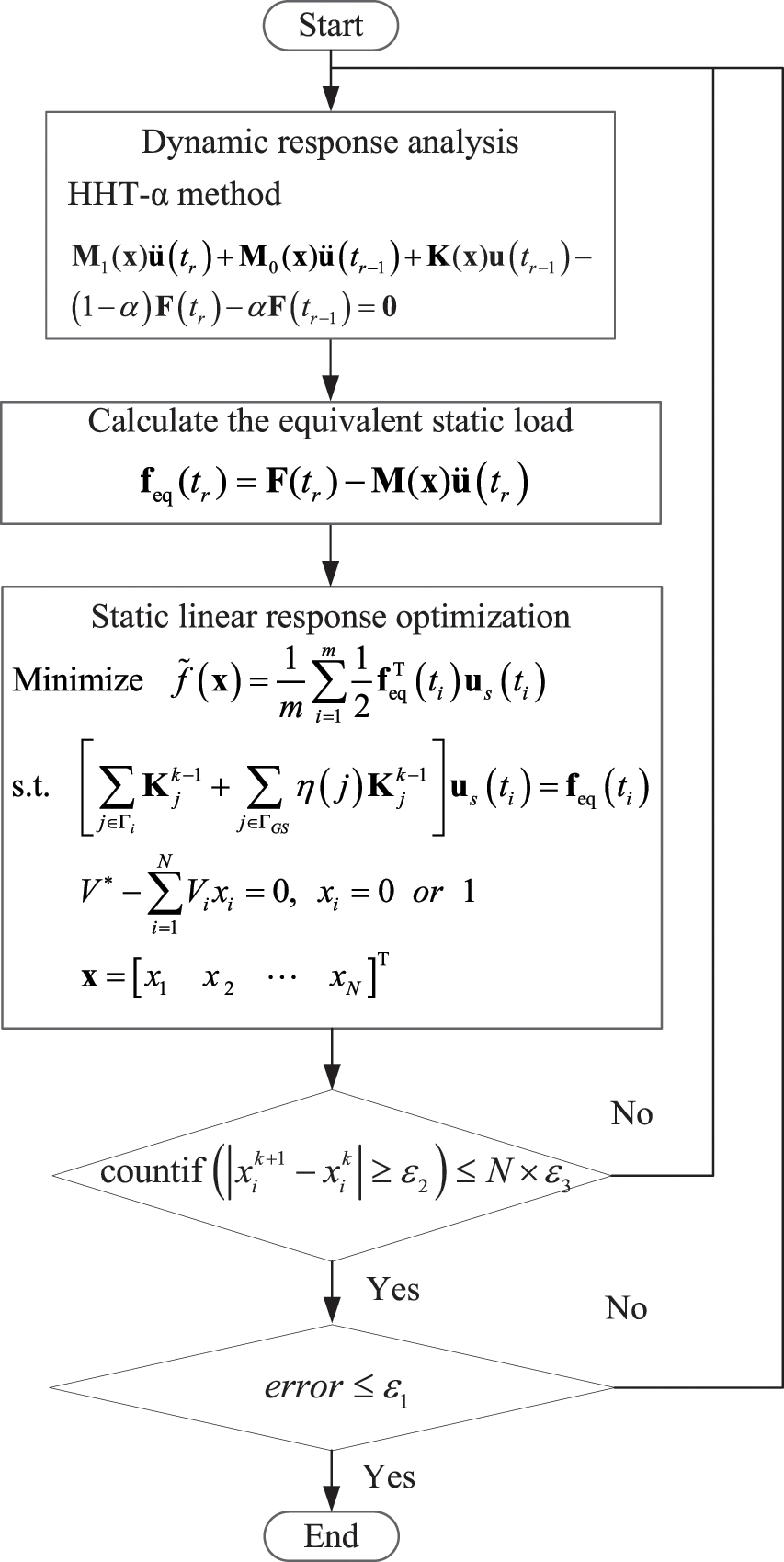
Figure 7: Dynamic compliance optimization process for a structure

Step. 1 Set the initial design variables and parameters.

Step. 2 Perform dynamic response analysis of a structure with respect to the design variables.

Step. 3 Compute the ESL sets at every time step.

Step. 4 Update the design variables according to sensitivity analysis using SBESO technique.

Step. 5 Once the convergent condition in (11) and (27) is simultaneously satisfied with given amount of material, the optimal process is terminated. Otherwise, go to Step 6.

Step. 6 Update the design, set k = k + 1, and go to Step 2.

4.4 Numerical Example

A long cantilever beam with dimensions 120 mm × 30 mm is depicted in Fig. 8a. The beam is subjected to a single dynamic load imposed at the middle point of right free edge, as illustrated in Fig. 8b. The design domain is meshed into 120 × 30 elements with an isoparametric 4-node. The objective volume fraction is prescribed to be 50%. The Young’s modulus of the material is E = 2 GPa, the Poisson’s ratio is μ = 0.3, and the mass density l is ρ = 4.8 × 103 Kg/m3. The weighted function is adopted as a linear function. The parameters of the SBESO algorithm are as follows: element removal rate is q = 60%–100%, convergence tolerance ɛ0 = ɛ1 = 0.001, ɛ2 = 0.3 and ɛ3 = 4%, sensitivity filtering radius rmin = 3 mm, and penalty factor p = 3.

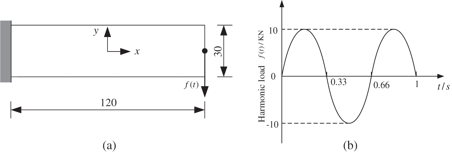
Figure 8: Long cantilever beam subjected to a single sinusoidal load (a) An initial design domain of a long cantilever beam (b) dynamic load

Fig. 9 shows the effect of element removal rate on the optimal topology and evolutionary process considering a single load case. It is found that BESO and SBESO procedures have almost the same mass distribution towards the clamped and free edges of the beam. Compared with the optimal topology from the BESO technique (q% = 100%), the SBESO scheme with the element removal rate of q% = 80% can obtain a better configuration with clearer and smoother borders while the BESO design has some areas with rough boundaries and undesirable islands. The unexpected island featured with small hole forms due to redundant element removal using the BESO technique. In addition, it is unfavorable for manufacturing. For the element removal rate of q% = 60%, additional beam-like members with nearly equal width are introduced to build the bridge between the clamped and free edges of the structure, which is greatly conducive to lessening the vertical deflection of the structure. Although the BESO method is convergent prior to the SBESO method, the latter provides the stable evolutionary history and has a slightly low value for mean dynamic compliance. The present example verifies that the SBESO method can achieve the optimal design of a structure with robust optimization process when compared with the BESO method. Most importantly, the presented numerical results demonstrate that the SESO technique base on the ESL method is efficient and robust in dynamic topology optimization problems in the time domain.

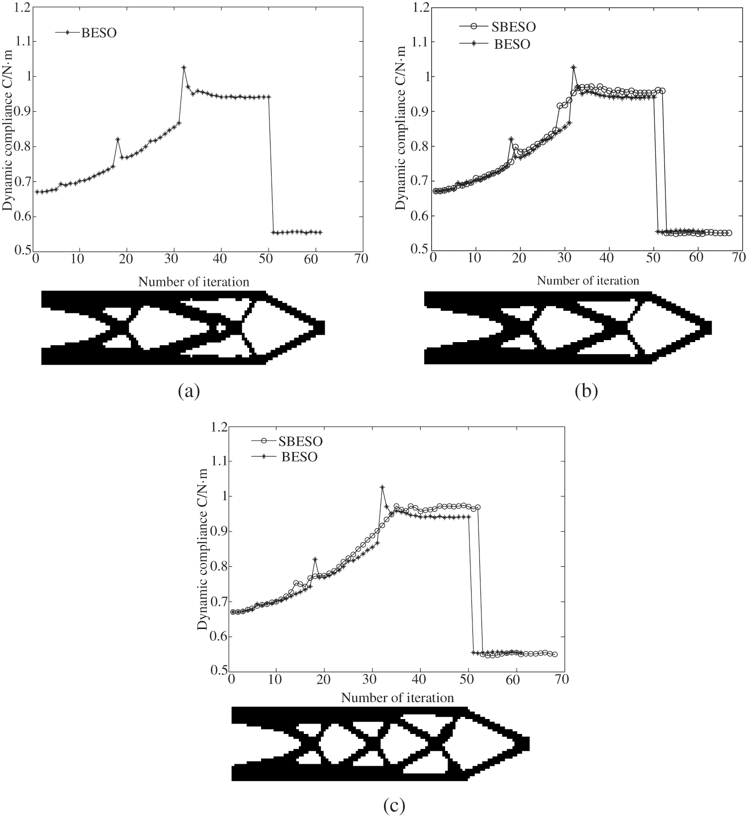
Figure 9: Effect of element removal rate on the optimal topology and convergence process for a long beam under a single sinusoidal load (a) q% = 100% (BESO) (b) q% = 80% (c) q% = 60%

Another example is shown in Fig. 10, where multiple load cases are considered for the dynamic optimization problem. All parameters for the structure and optimization are identical to those used for the single load case as illustrated in Fig. 8. For multiple load cases, the optimization problem can be formulated as minimization of total dynamic compliance caused by each load. As such the optimization problem considering multiple load cases can be defined as follows

Minimize C∼(x)=∑l=121m∑r=1m12feq,lTus(tr)s.t.  V∗−∑i=1NVixi=0   M(x)u..(tr)+K(x)u(tr)=Fl(tr)   feq,l(tr)=Fl(tr)−M(x)u..(tr)   K(x)us(tr)=feq,l(tr)(r=1,…,m;l=1,2)   xi=0or1(i=1,…,N)(28)

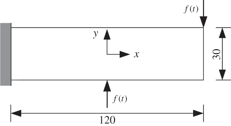
Figure 10: Long cantilever beam subjected to multiple load cases

The resulting optimized solution together with convergent history using BESO scheme is presented in Fig. 11a, while the resulting improved solutions together with convergent history using SBESO scheme in Figs. 11b and 11c under multiple load cases. It is noted that the topology obtained from BESO scheme is significantly different from those obtained from SBESO scheme aside from right part of design domain. The dynamic compliance of the BESO solution (q% = 100%) and SBESO solution (q% = 80% and q% = 60%) are equal to 0.316, 0.292 and 0.281 Nm, respectively. Thus, the dynamic compliance decrease for SBESO scheme are 7.6% in the scenario of q% = 80% and 11.1% in the scenario of q% = 60% relative to that for BESO scheme. It can attribute to the fact that the SBESO solutions provide relatively thick beam-like members. It is evident that the optimized topology obtained from SBESO scheme with element removal rate of 60% is preferable due to higher dynamic stiffness and smoother boundary.

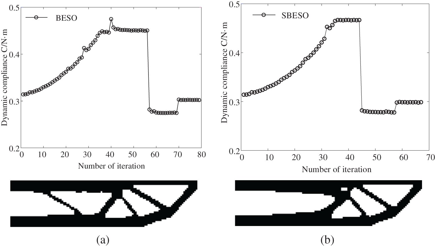
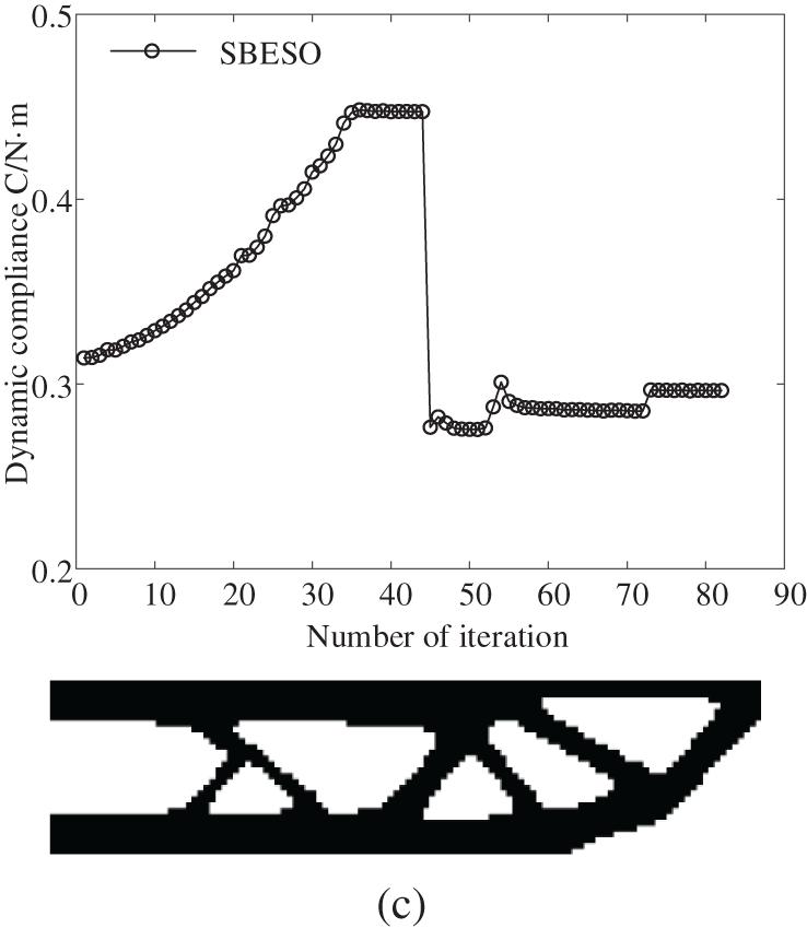
Figure 11: Effect of element removal rate on the optimal topology and convergence process for a long beam under multiple load cases (a) q% = 100% (BESO) (b) q% = 80% (c) q% = 60%

5  Conclusion

In this study, we propose a variant of SESO, called SBESO, to solve the topology optimization of eigenfrequency and dynamic compliance in the time domain. The SBESO technique is based on the philosophy that the unnecessary region for a structure has the corresponding elements smoothly removed by gradually reducing those stiffness and mass matrixes. The main observations of this study are as follows:

•   Various weighted functions significantly influence the optimal process and configuration. Among the analyzed weighted functions, the sine and linear function yield the smoother iterative history while the constant function is a more radical one. It seems that the smooth weighted function contributes to regulating the optimal process.

•   The element removal rate is a key parameter in dynamic optimization, because a low value results in a high computational burden and a high value instability in the structure due to the overdue removal of elements in a single iteration. This element removal rate functions similarly to the step size in mathematical programming influencing the optimal process.

•   The element removal occurs smoothly using the SBESO procedure, not radically as the classic BESO behaves. The benchmark examples indicated that SBESO can generate efficient structure form and smooth boundary for continuum structures in contrast to those produced by the BESO method.

Therefore, it is anticipated that the development of the present SBESO technique for free and forced vibration problems can tackle dynamic topology optimization of continuum structures in an effective and powerful way.

Funding Statement: This study was supported by the National Natural Science Foundation of China (Grant No. 51505096), and the Natural Science Foundation of Heilongjiang Province (Grant No. LH2020E064).

Conflicts of Interest: The authors declare that they have no conflicts of interest to report regarding the present study.

References

1. Mendes, E., Sivapuram, R., Rodriguez, R., Sampaio, M., Picelli, R. (2022). Topology optimization for stability problems of submerged structures using the TOBS method. Computers & Structures, 259, 106685. DOI 10.1016/j.compstruc.2021.106685. [Google Scholar] [CrossRef]
2. Wang, Y., Lei, R., Wang, H. (2022). Structural topology optimization of flying wing aircraft. Journal of Beijing University of Aeronautics and Astronautics, 48, 1–13. [Google Scholar]
3. Zhang, Y., Shan, Y., Liu, X., He, T. (2021). An integrated multi-objective topology optimization method for automobile wheels made of lightweight materials. Structural and Multidisciplinary Optimization, 64(3), 1585–1605. DOI 10.1007/s00158-021-02913-3. [Google Scholar] [CrossRef]
4. Zargham, S., Ward, T. A., Ramli, R., Badruddin, I. A. (2016). Topology optimization: A review for structural designs under vibration problems. Structural and Multidisciplinary Optimization, 53(6), 1157–1177. DOI 10.1007/s00158-015-1370-5. [Google Scholar] [CrossRef]
5. Kuang, B., Li, Y., Liu, F., Liu, J. (2016). Bidirectional evolutionary structural optimization method based on control for evolutionary step length of element density. Chinese Journal of Computational Mechanics, 33(1), 15–21. [Google Scholar]
6. Almeida, V. S., Simonetti, H. L., Neto, L. O. (2013). Comparative analysis of strut-and-tie models using smooth evolutionary structural optimization. Engineering Structures, 56, 1665–1675. DOI 10.1016/j.engstruct.2013.07.007. [Google Scholar] [CrossRef]
7. Simonetti, H. L., Almeida, V. S., de Oliveira Neto, L. (2014). A smooth evolutionary structural optimization procedure applied to plane stress problem. Engineering Structures, 75, 248–258. DOI 10.1016/j.engstruct.2014.05.041. [Google Scholar] [CrossRef]
8. Simonett, H. L., Almeid, V. S., das Neves, F. D. A. (2019). Topology optimization: Compliance minimization using SESO with bilinear square element. London Journal of Engineering Research, 19(1), 33–39. [Google Scholar]
9. Fernandes, W. S., Almeida, V. S., Neves, F. A., Greco, M. (2015). Topology optimization applied to 2D elasticity problems considering the geometrical nonlinearity. Engineering Structures, 100, 116–127. DOI 10.1016/j.engstruct.2015.05.042. [Google Scholar] [CrossRef]
10. Fernandes, W. S., Greco, M., Almeida, V. S. (2017). Application of the smooth evolutionary structural optimization method combined with a multi-criteria decision procedure. Engineering Structures, 143, 40–51. DOI 10.1016/j.engstruct.2017.04.001. [Google Scholar] [CrossRef]
11. Mukherjee, S., Lu, D., Raghavan, B., Breitkopf, P., Dutta, S. et al. (2021). Accelerating large-scale topology optimization: State-of-the-art and challenges. Archives of Computational Methods in Engineering, 28(7), 4549–4571. DOI 10.1007/s11831-021-09544-3. [Google Scholar] [CrossRef]
12. Huang, X., Zuo, Z. H., Xie, Y. M. (2010). Evolutionary topological optimization of vibrating continuum structures for natural frequencies. Computers & Structures, 88(5–6), 357–364. DOI 10.1016/j.compstruc.2009.11.011. [Google Scholar] [CrossRef]
13. Wang, Y., Qin, D., Wang, R., Zhao, H. (2021). Dynamic topology optimization of long-span continuum structures. Shock and Vibration, 2021, 1–9. DOI 10.1155/2021/4421298. [Google Scholar] [CrossRef]
14. Leader, M. K., Chin, T. W., Kennedy, G. J. (2019). High-resolution topology optimization with stress and natural frequency constraints. AIAA Journal, 57(8), 3562–3578. DOI 10.2514/1.J057777. [Google Scholar] [CrossRef]
15. Li, Q., Wu, Q., Liu, J., He, J., Liu, S. (2021). Topology optimization of vibrating structures with frequency band constraints. Structural and Multidisciplinary Optimization, 63(3), 1203–1218. DOI 10.1007/s00158-020-02753-7. [Google Scholar] [CrossRef]
16. Silva, O. M., Neves, M. M., Lenzi, A. (2019). A critical analysis of using the dynamic compliance as objective function in topology optimization of one-material structures considering steady-state forced vibration problems. Journal of Sound and Vibration, 444, 1–20. DOI 10.1016/j.jsv.2018.12.030. [Google Scholar] [CrossRef]
17. Niu, B., He, X., Shan, Y., Yang, R. (2018). On objective functions of minimizing the vibration response of continuum structures subjected to external harmonic excitation. Structural and Multidisciplinary Optimization, 57(6), 2291–2307. DOI 10.1007/s00158-017-1859-1. [Google Scholar] [CrossRef]
18. Tuncer, G., Sendur, P. (2020). Frequency-based dynamic topology optimization methodology for improved door closing sound quality. Proceedings of the Institution of Mechanical Engineers, Part C: Journal of Mechanical Engineering Science, 234(7), 1311–1322. [Google Scholar]
19. Martin, A., Deierlein, G. G. (2020). Structural topology optimization of tall buildings for dynamic seismic excitation using modal decomposition. Engineering Structures, 216, 110717. DOI 10.1016/j.engstruct.2020.110717. [Google Scholar] [CrossRef]
20. Yun, K. S., Youn, S. K. (2018). Topology optimization of viscoelastic damping layers for attenuating transient response of shell structures. Finite Elements in Analysis and Design, 141, 154–165. DOI 10.1016/j.finel.2017.12.003. [Google Scholar] [CrossRef]
21. Giraldo-Londoño, O., Paulino, G. H. (2021). PolyDyna: A matlab implementation for topology optimization of structures subjected to dynamic loads. Structural and Multidisciplinary Optimization, 64(2), 957–990. DOI 10.1007/s00158-021-02859-6. [Google Scholar] [CrossRef]
22. Huang, G., Chen, X., Yang, Z. (2018). A modified gradient projection method for static and dynamic topology optimization. Engineering Optimization, 50(9), 1515–1532. DOI 10.1080/0305215X.2017.1410146. [Google Scholar] [CrossRef]
23. Sun, J., Tian, Q., Hu, H. (2018). Topology optimization of a three-dimensional flexible multibody system via moving morphable components. Journal of Computational and Nonlinear Dynamics, 13(2), 1–34. DOI 10.1115/1.4038142. [Google Scholar] [CrossRef]
24. Park, S. O., Choi, W. H., Park, G. J. (2021). Dynamic response optimization of structures with viscoelastic material using the equivalent static loads method. Proceedings of the Institution of Mechanical Engineers, Part D: Journal of Automobile Engineering, 235(2–3), 589–603. [Google Scholar]
25. Stolpe, M. (2014). On the equivalent static loads approach for dynamic response structural optimization. Structural and Multidisciplinary Optimization, 50(6), 921–926. DOI 10.1007/s00158-014-1101-3. [Google Scholar] [CrossRef]
Cite This Article
Copyright © 2023 The Author(s). Published by Tech Science Press.
This work is licensed under a Creative Commons Attribution 4.0 International License , which permits unrestricted use, distribution, and reproduction in any medium, provided the original work is properly cited.
Downloads
Citation Tools