
 Submit a Paper
 Propose a Special lssue
 Open Access
ARTICLE

A Novel Modified Alpha Power Transformed Weibull Distribution and Its Engineering Applications
1 Department of Mathematical Sciences, College of Science, Princess Nourah bint Abdulrahman University, P.O. Box 84428, Riyadh, 11671, Saudi Arabia
2 Department of Statistics, Faculty of Science, King Abdulaziz University, Jeddah, 80200, Saudi Arabia
3 Department of Mathematics, Faculty of Science, Al-Azhar University, Nasr City, Cairo, 11884, Egypt
4 Department of Statistics, Faculty of Commerce, Zagazig University, Zagazig, 44519, Egypt
5 Faculty of Technology and Development, Zagazig University, Zagazig, 44519, Egypt
* Corresponding Author: Ahmed Elshahhat. Email:
(This article belongs to the Special Issue: New Trends in Statistical Computing and Data Science)
Computer Modeling in Engineering & Sciences 2023, 135(3), 2065-2089. https://doi.org/10.32604/cmes.2023.023408
Received 24 April 2022; Accepted 11 July 2022; Issue published 23 November 2022
 View Full Text
 Download PDF
Abstract
This paper suggests a new modified version of the traditional Weibull distribution by adding a new shape parameter utilising the modified alpha power transformed technique. We refer to the new model as modified alpha power transformed Weibull distribution. The attractiveness and significance of the new distribution lie in its power to model monotone and non-monotone failure rate functions, which are quite familiar in environmental investigations. Its hazard rate function can be decreasing, increasing, bathtub and upside-down then bathtub shaped. Diverse structural properties of the proposed model are acquired including quantile function, moments, entropies, order statistics, residual life and reversed failure rate function. The parameters of the distribution were estimated using the maximum likelihood function. The maximum likelihood method is employed to estimate the model parameters and the approximate confidence intervals are also computed. Via a simulation study, the performance of the point and interval estimates are compared using different criteria. Employing real lifetime data sets, we verify that the offered model furnishes a better fit than some other lifetime models including Weibull, gamma and alpha power Weibull models.Keywords
The Weibull distribution is a wildly favoured lifetime distribution in reliability studies. It is naturally employed for studying biological, hydrological and medical data sets. The Weibull distribution is frequently employed as a suitable alternative to well-known distributions such as exponential, gamma and inverse Weibull distributions. The random variable X is expressed to have a Weibull distribution if its probability density function (PDF) is given by
where
One of the major weaknesses of the Weibull distribution is that it does not deliver an adequate fit for some applications, particularly, when the hazard rates are upside-down bathtub or bathtub shapes. To overcome this disadvantage, several investigators have developed various generalizations and modifications of the Weibull distribution to model different types of data in recent years. The generalized Weibull distribution was introduced in reference [1,2] by adding a shape parameter to the Weibull distribution. Likewise, Xie et al. [3] proposed the additive Weibull distribution, the generalized modified Weibull distribution by [4], KumaraswamyWeibull distribution by [5], beta Sarhan-Zaindin modified Weibull distribution by [6], Weibull-Weibull distribution by [7], alpha power Weibull (APW) distribution by [8], log-normal modified Weibull distribution and its reliability implications by [9], generalized extended exponential-Weibull distribution by [10], Poisson modified weibull distribution by [11], alpha logarithmic transformed Weibull distribution by [12] and logarithmic transformed Weibull by [13].
Recently, Mahdavi et al. [14] suggested a new approach to present an additional parameter to a class of distributions for more additional flexibility. The offered technique is named alpha power transformation (APT) and it is worthwhile to incorporate skewness into a family of distributions. They studied the main properties of the APT method and introduced an extension to the exponential distribution using the new approach. Many authors used the same technique to introduce new generalizations of some well-known distribution. For example, alpha power Weibull distribution by [8], alpha power generalized exponential by [15], alpha power transformed inverse Lindley distribution by [16] and alpha power Gompertz distribution by [17]. To add more flexibility to the APT method, Alotaibi et al. [18] proposed a new form of the APT method which is called the modified APT (MAPT) method. The CDF and the PDF of the MAPT method are, respectively, given by
and
where
Modelling real data employing generalized distributions stays vital nowadays. Multiple generalized distributions have been considered and used in different domains. Nevertheless, there still remain considerable necessary issues applying real data, which are not handled by available models. The main purpose of this article is to offer a new unexplored version of the traditional Weibull distribution. To achieve this goal, we utilize the MAPT method to add a new shape parameter to the baseline CDF given by (2). We refer to the new model as modified alpha power transformed Weibull (MAPTW) distribution which contains one scale and two shape parameters. The main properties of the new model including, quantile, mixture expansion, moments, entropies and order statistics are derived. The unknown parameters are estimated using the maximum likelihood estimation method and the approximate confidence intervals (ACIs) of the unknown parameters are also constructed. We are encouraged to introduce the MAPTW distribution because
1. It contains some well-known distributions as special cases including, exponential, Weibull and MAPT exponential (MAPTE) distributions. So, at least, the MAPTW distribution contains the main properties of these important distributions which are commonly used in modelling lifetime data. Also, the main characteristics of these distributions can be obtained directly from the MAPTW distribution.
2. It is appropriate to model positively skewed, negatively skewed and approximately symmetric data which may not be adequately modelled by other competitive models.
3. It can model decreasing, increasing, bathtub and upside-down then bathtub hazard rates which are often faced in real-life problems.
4. It is indicated in Section 2 that the MAPTW distribution can be shown as a combination of the Weibull distribution. This property is especially helpful to derive the properties of the MAPTW distribution directly from the Weibull distribution.
5. The analysis of two real data sets demonstrate that the MAPTW distribution compares satisfactorily with different competing lifetime distributions in modelling engineering data sets. As a results, the MAPTW distribution can be able to model engineering applications rather that some well known and recently proposed generalized models. This is due to the flexibility of its PDF and hazard rate function (HRF).
One of the main advantages of this distribution over many other generalized distributions is that it gives the main forms of the HRF with two shape parameters only. The same advantage can be found in its PDF which can be used to model positively and negatively skewed as well as approximately symmetric data which may not be adequately fitted by other distributions. This makes the new distribution more flexible, especially for modelling data sets when studying reliability experiments, electronics, materials, automotive industries and many engineering applications. Another motivation for this study is examining the behaviour of the maximum likelihood estimators as well as the ACIs by considering different sample sizes and different true parameter values. The rest of the paper is classified as follows: We present the MAPTW distribution in Section 2. The main properties of the MAPTW distribution are derived in Section 3. In Section 4, we discuss the maximum likelihood estimates (MLEs) as well as the ACIs of the model parameter. In Section 5, a simulation study is conducted to compare the performance of point and interval estimates. The effectiveness of the MAPTW distribution is depicted by studying two real data sets from the engineering field in Section 6. Finally, in Section 7 we conclude the paper.
2 The Modified Alpha Power Transformed Weibull Distribution
The MAPTW distribution is discussed in this section. If X has a Weibull distribution with PDF and CDF, respectively, provided by (1) and (2), then the CDF of the MAPTW distribution is given by (3).
and the corresponding PDF is given by
where
and
Henceforward, X is used to denote the random variable that has the PDF in (6). Fig. 1 shows the various forms of the PDF of the MAPTW distribution given by (6) by assuming different values of the shape parameters and by considering the scale parameter

Figure 1: Plots for the PDF of the MAPTW distribution

Figure 2: Plots for the HRF of the MAPTW distribution
To derive the main properties of the MAPTW distribution, we provide a valuable expansion for the PDF in (6). Consider the following power series:
and the generalized binomial expansion in the form
Using the series in (9) and (10), one can write the PDF in (6) as a mixture representation of the Weibull densities as follows:
where
Moreover, we can write the linear representation of the CDF of the MAPTW distribution after integrating (11), as follows:
where
We provide some essential properties for the MAPTW distribution in this section, such as quantile, moments, entropies, order statistics, residual life, and reversed failure rate function.
The quantile function (QF) of the MAPTW distribution, say
The QF in (13) can be used to generate a random sample from the MAPTW distribution by taking p to be
Moments play an essential feature in statistical theory and numerous necessary characteristics of any distribution can be examined via moments. For the MAPTW distribution, the
where
Practically, the mean of the MAPTW distribution can be obtained from (14) by setting
Similarly, the second moment can be obtained by putting
Then, once can obtain the variance of the MAPTW distribution using the following relation:
The
and
where

Figure 3: Mean, variance, skewness and kurtosis of the MAPTW distribution
The following Lemma explain various kinds of moments of the MAPTW distribution such as incomplete moments (IMs), moment generating function (MGF), characteristic generating function (CGF) and conditional moments (CMs).
Lemma 3.1. If X
1. The IMs of X is
where
2. The MGF of X is
3. The CGF of X is
4. The CMs of X is
Entropy is one of the numerous popular techniques used to calculate the uncertainty corresponding to a random variable and it was initially employed in the field of physics. Estimating entropy is a significant matter in many fields including statistics and biological phenomenon. High entropy is guided to minor information found in data. For the MAPTW distribution and from (6), the Renyi entropy (RE) can be acquired as follows:
Also, Shannon’s entropy can be derived by Limiting
Order statistics contain a broad range of applications in statistics, including nonparametric statistics, life testing, quality control monitoring and reliability analysis. Let
where B(.,.) is the beta function. Using (5), (6) and a power series expansion, we obtain
Substituting (17) in Eq. (16), the PDF of
where
3.5 Probability Weighted Moments
The
For the of the MAPTW distribution, it follows from (5) and (6) that
Substituting (20) in Eq. (19), the probability weighted moments of the MAPTW distribution is given by
3.6 Residual Life and Reversed Failure Rate Function
The
Using (6) and applying the binomial expansion of
where
where
Using (5), (6) and applying the binomial expansion of
Let
Case one: When
Using the series expansion in (10), the last equation takes the form
Employing the series expansion in (9), we obtain
where
and
Case two: When
Let
Using the series expansion in (10), we have
Utilizing the series expansion in (9), it comes
where
and
4 Estimation of the Parameters
Here, the method of maximum likelihood is employed to estimate the unknown parameters of the MAPTW distribution. Moreover, the approximate confidence intervals (ACIs) of the unknown parameters are obtained. Assume that we have a random sample of size n taken from the MAPTW distribution with PDF given by (6), then we can express the log-likelihood function in this case as follows:
To get the maximum likelihood estimates (MLEs) of
and
where
and
It is to note that there are no closed-form solutions for Eqs. (22)–(24). To get the MLEs in this case, one can direct to any numerical technique for this purpose. Using the asymptotic properties of the MLEs, we can obtain the ACIs of
where
and
where
Thus, the
where
To evaluate the performance of the MLEs of the MAPTW distribution, a Monte Carlo simulation is conducted based on a sufficiently large 5,000 independent from the MAPTW distribution using different sample sizes
Step 1: Determine the sample size and the starting values for the parameters.
Step 2: Generate a random sample of size n from the MAPTW distribution from (9).
Step 3: Compute the average estimates with their root mean squared-errors (RMSEs) and relative absolute biases (RABs) of
Step 4: Obtain the
Step 5: Repeat steps 2–5 5000 times.
Step 6: Calculate the average values (AV) of MLEs, RMSEs, RABs and CLs of any function of
and
where
All required numerical results are obtained via
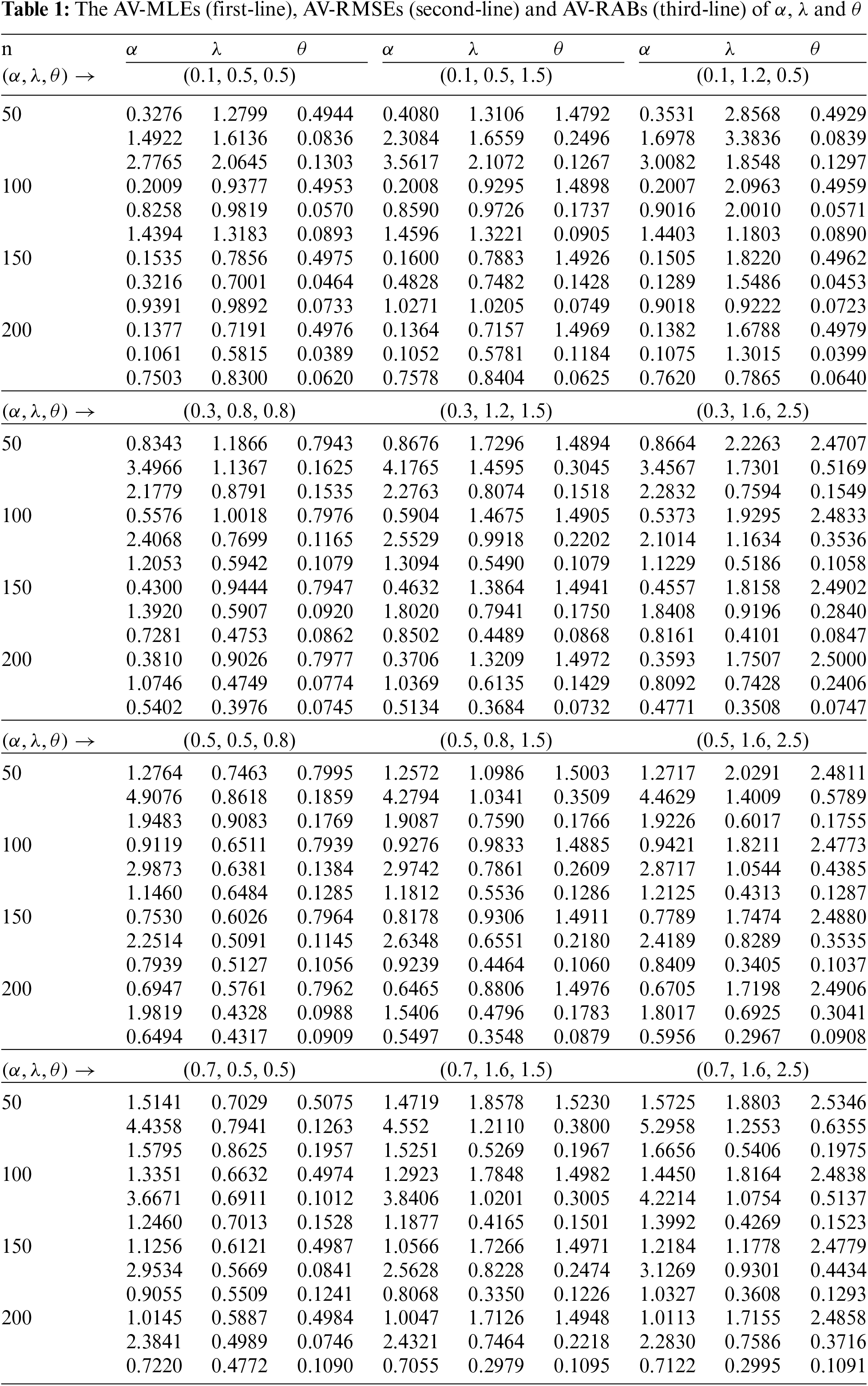
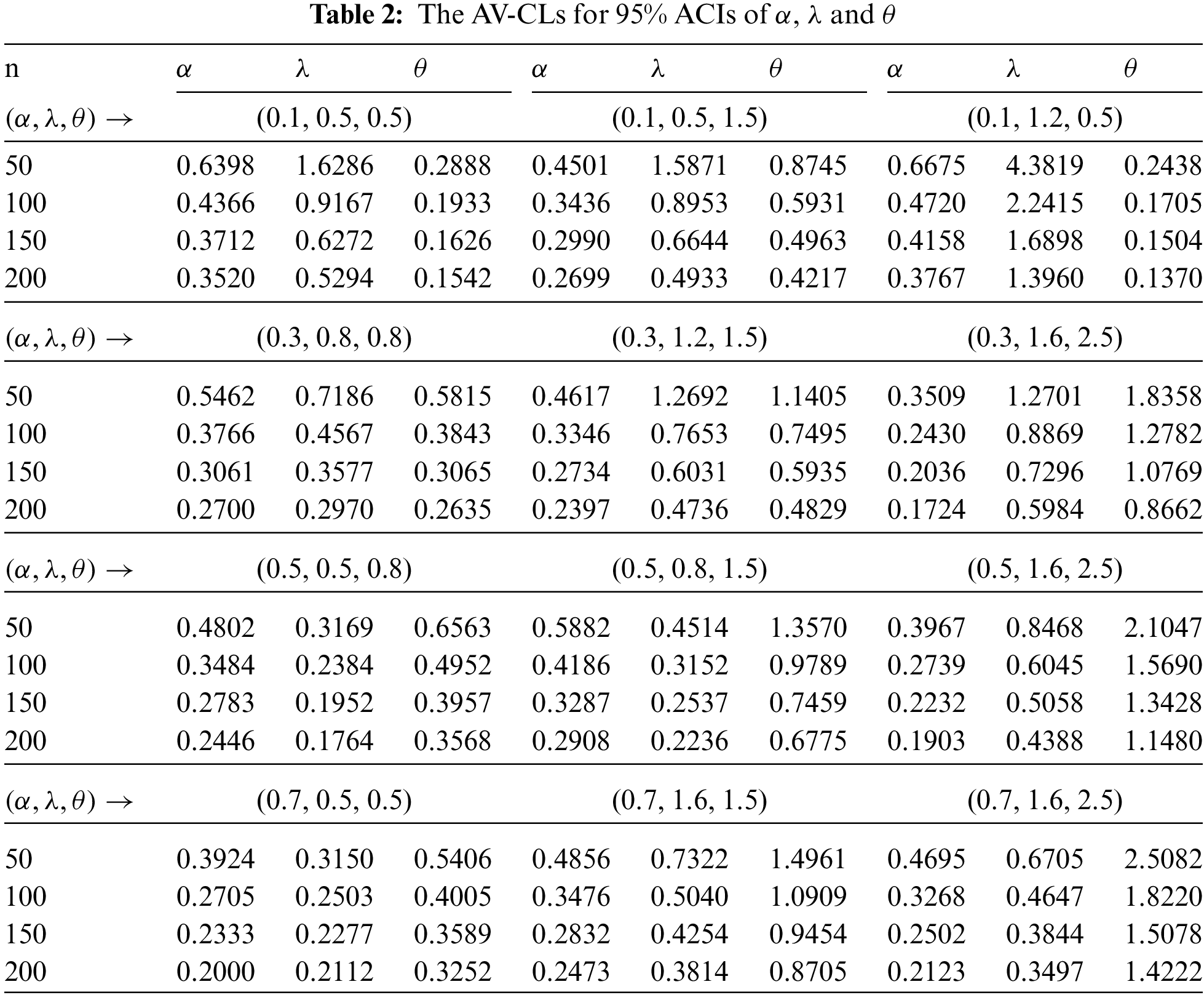

Figure 4: Plot of the RMSEs, RABs (left-panel) and CLs (right-panel) of
To show how our proposed model works in practice, in this section we present the analysis of two real data sets from engineering science for illustrative purposes. The first data set (denoted by Data-I) consists of 40 observations of the active repair times for airborne communication transceiver, see [22]. The second data set (denoted by Data-II) represents the failure times of 84 Aircraft Windshields and been obtained from [23]. The values of both data sets I and II are arranged with ascending order and reported in Table 3.

First, to identify the shape of the HRF of MAPTW distribution, we shall consider a graphical method, given by [24], based on the total time on test (TTT) plot. However, the scaled TTT transform based on both observed data sets I and II is given by

Figure 5: Empirical and estimated scaled TTT-transform plot of the MAPTW distribution
To monitored the applicability and flexibility of the MAPTW distribution, we compare fit the MAPTW distribution to both data sets I and II with several other competitive models exhibiting various hazard rates, namely: alpha power transformed generalized-exponential (APTGE), alpha power exponential (APE), APW, generalized-exponential (GE), Nadarajah-Haghighi (NH), gamma (G) and Weibull (W) distributions. The corresponding PDFs of the competing models (for

To show the feasibility and validity of the MAPTW model along with other seven competing models, several goodness-of-fit measures namely; estimated negative log-likelihood (NL), Akaike information criterion (AIC), consistent Akaike information criterion (CAIC), Bayesian information criterion (BIC) and Hannan-Quinn information criterion (HQIC) are considered. Based on both data sets I and II, the selection criteria as well as the MLEs along with their standard errors (SEs) of the model parameters are calculated and provided in Table 5. It shows that the MAPTW distribution has the smallest values of NCL, AIC, CAIC, BIC, HQIC, K-S and the highest P-value. Moreover, Fig. 6 shows graphically the quantile-quantile (QQ) plots of all competitive distributions for given data sets. Furthermore, the relative histograms of both data sets and the fitted densities, as well as the fitted/empirical survival functions, are plotted in Fig. 7. It can be seen from Figs. 6 and 7, that the graphical presentations support the same numerical findings presented in Table 5. Thus, the proposed MAPTW distribution provides the best fit, for the given data sets, than the APTGE, APTW and other popular lifetime distributions. Since the empirical HRFs of the two data sets are decreasing and increasing, respectively, and most of the competitive models such as Weibull and APW distributions can model such HRFs, the results show that the MAPTW distribution provides a better fit for the two engineering applications in terms of goodness of fit statistics. This is because the MAPTW distribution has a very flexible HRF with different shape behaviour as well as a flexible PDF, especially for skewed data. To sum up, we recommend the use of MAPTW for real practical purposes.


Figure 6: The QQ plots of MAPTW distribution and its competing models for Data-I and Data-II

Figure 7: Histogram and fitted densities (left panel), empirical and fitted survival functions (right panel) of MAPTW distribution and some competing models
In this paper, we have offered a fresh version of Weibull distribution named the modified alpha power transformed Weibull distribution. The proposed distribution is acquired by taking the Weibull distribution as the baseline distribution in the modified alpha power transformed method. Some properties of the new distribution are derived. The hazard rate function of the new distribution can take different shapes possessing decreasing, increasing, bathtub and upside-down then bathtub shaped. Accordingly, it can be viewed perfectly effectively in modelling lifetime data. Via the maximum likelihood method, the point and interval estimates of the model parameters are evaluated. The performance of the point and interval estimates is assessed through a simulation study. The simulation yields verified that the estimates are asymptotically unbiased and consistent. In addition, two real data sets to active repair times for airborne communication transceiver and the failure times of aircraft windshields are investigated. From the empirical results, we can conclude that the new distribution provides a more adequate fit than some known distributions including gamma, Weibull and alpha power Weibull distributions. For future work, it is of interest to study the proposed distribution under different censoring schemes including Type-II and progressive Type-II censoring. Another future work is to investigate the Bayesian estimation of the unknown parameters of the suggested model.
Acknowledgement: The authors would like to thank the Editor, Assistant Editor and Reviewers for their constructive recommendations which assisted us to improve the manuscript. The authors extend their appreciations to Princess Nourah bint Abdulrahman University Researchers Supporting Project No. (PNURSP2022R50), Princess Nourah bint Abdulrahman University, Riyadh, Saudi Arabia.
Funding Statement: This research was funded by Princess Nourah bint Abdulrahman University Researchers Supporting Project No. (PNURSP2022R50), Princess Nourah bint Abdulrahman University, Riyadh, Saudi Arabia.
Conflicts of Interest: The authors declare that they have no conflicts of interest to report regarding the present study.
References
1. Mudholkar, G. S., Srivastava, D. K., Friemer, M. (1995). The exponentiated weibull family: A reanalysis of the bus-motor-failure data. Technometrics, 37, 436–445. DOI 10.1080/00401706.1995.10484376. [Google Scholar] [CrossRef]
2. Mudholkar, G. S., Srivastava, D. K., Kollia, G. D. (1996). A generalization of the weibull distribution with application to the analysis of survival data. Journal of the American Statistical Association, 91(436), 1575–1583. DOI 10.1080/01621459.1996.10476725. [Google Scholar] [CrossRef]
3. Xie, M., Lai, C. D. (1996). Reliability analysis using an additive weibull model with bathtub-shaped failure rate function. Reliability Engineering & System Safety, 52(1), 87–93. DOI 10.1016/0951-8320(95)00149-2. [Google Scholar] [CrossRef]
4. Carrasco, J. M., Ortega, E. M., Cordeiro, G. M. (2008). A generalized modified weibull distribution for lifetime modeling. Computational Statistics & Data Analysis, 53(2), 450–462. DOI 10.1016/j.csda.2008.08.023. [Google Scholar] [CrossRef]
5. Cordeiro, G. M., Ortega, E. M., Nadarajah, S. (2010). The kumaraswamy weibull distribution with application to failure data. Journal of the Franklin Institute, 347(8), 1399–1429. DOI 10.1016/j.jfranklin.2010.06.010. [Google Scholar] [CrossRef]
6. Saboor, A., Bakouch, H. S., Khan, M. N. (2016). Beta sarhan-zaindin modified weibull distribution. Applied Mathematical Modelling, 40(13–14), 6604–6621. DOI 10.1016/j.apm.2016.01.033. [Google Scholar] [CrossRef]
7. Abouelmagd, T. H. M., Al-mualim, S., Elgarhy, M., Afify, A. Z., Ahmad, M. (2018). Properties of the four-parameter weibull distribution and its applications. Pakistan Journal of Statistics, 33, 449–466. [Google Scholar]
8. Nassar, M., Alzaatreh, A., Mead, M., Abo-Kasem, O. (2017). Alpha power weibull distribution: Properties and applications. Communications in Statistics-Theory & Methods, 46(20), 10236–10252. DOI 10.1080/03610926.2016.1231816. [Google Scholar] [CrossRef]
9. Shakhatreh, M. K., Lemonte, A. J., Moreno–Arenas, G. (2019). The log-normal modified weibull distribution and its reliability implications. Reliability Engineering & System Safety, 188, 6–22. DOI 10.1016/j.ress.2019.03.014. [Google Scholar] [CrossRef]
10. Shakhatreh, M. K., Lemonte, A. J., Cordeiro, G. M. (2020). On the generalized extended exponential-weibull distribution: Properties and different methods of estimation. International Journal of Computer Mathematics, 97(5), 1029–1057. DOI 10.1080/00207160.2019.1605062. [Google Scholar] [CrossRef]
11. Abd El-Monsef, M. M. E., Marei, G. A., Kilany, N. M. (2022). Poisson modified Weibull distribution with inferences on stress-strength reliability model. Quality & Reliability Engineering International, 38(5), 2649–2669. DOI 10.1002/qre.3096. [Google Scholar] [CrossRef]
12. Nassar, M., Afify, A. Z., Dey, S., Kumar, D. (2018). A new extension of weibull distribution: Properties and different methods of estimation. Journal of Computational & Applied Mathematics, 336, 439–457. DOI 10.1016/j.cam.2017.12.001. [Google Scholar] [CrossRef]
13. Nassar, M., Afify, A. Z., Shakhatreh, M. K., Dey, S. (2020). On a new extension of weibull distribution: Properties, estimation, and applications to one and two causes of failures. Quality & Reliability Engineering International, 36(6), 2019–2043. DOI 10.1002/qre.2671. [Google Scholar] [CrossRef]
14. Mahdavi, A., Kundu, D. (2017). A new method for generating distributions with an application to exponential distribution. Communications in Statistics-Theory & Methods, 46(13), 6543–6557. DOI 10.1080/03610926.2015.1130839. [Google Scholar] [CrossRef]
15. Dey, S., Alzaatreh, A., Zhang, C., Kumar, D. (2017). A new extension of generalized exponential distribution with application to ozone data. Ozone: Science & Engineering, 39(4), 273–285. DOI 10.1080/01919512.2017.1308817. [Google Scholar] [CrossRef]
16. Dey, S., Nassar, M., Kumar, D. (2019). Alpha power transformed inverse lindley distribution: A distribution with an upside-down bathtub-shaped hazard function. Journal of Computational & Applied Mathematics, 348, 130–145. DOI 10.1016/j.cam.2018.03.037. [Google Scholar] [CrossRef]
17. Eghwerido, J. T., Nzei, L. C., Agu, F. I. (2021). The alpha power gompertz distribution: Characterization, properties, and applications. Sankhya A, 83(1), 449–475. DOI 10.1007/s13171-020-00198-0. [Google Scholar] [CrossRef]
18. Alotaibi, R., Okasha, H., Rezk, H., Nassar, M. (2021). A new weighted version of alpha power transformation method: Properties and applications to COVID-19 and software reliability data. Physica Scripta, 96, 125–221. DOI 10.1088/1402-4896/ac2658. [Google Scholar] [CrossRef]
19. Henningsen, A., Toomet, O. (2011). maxLik: A package for maximum likelihood estimation in R. Computational Statistics, 26(3), 443–458. DOI 10.1007/s00180-010-0217-1. [Google Scholar] [CrossRef]
20. Elshahhat, A., Elemary, B. R. (2021). Analysis for xgamma parameters of life under type-II adaptive progressively hybrid censoring with applications in engineering and chemistry. Symmetry, 13(11), 2112. DOI 10.3390/sym13112112. [Google Scholar] [CrossRef]
21. Elshahhat, A., Aljohani, H. M., Afify, A. Z. (2021). Bayesian and classical inference under type-II censored samples of the extended inverse gompertz distribution with engineering applications. Entropy, 23(12), 1578. DOI 10.3390/e23121578. [Google Scholar] [CrossRef]
22. Jorgensen, B. (1982). Statistical properties of the generalized inverse gaussian distribution. New York, USA: Springer. [Google Scholar]
23. Murthy, D. N. P., Xie, M., Jiang, R. (2004). Weibull models. Wiley, Hoboken: Wiley Series in Probability & Statistics. [Google Scholar]
24. Aarset, M. V. (1987). How to identify a bathtub hazard rate. IEEE Transactions on Reliability, 36, 106–108. DOI 10.1109/TR.1987.5222310. [Google Scholar] [CrossRef]
25. Weibull, W. (1951). A statistical distribution function of wide applicability. Journal of Applied Mechanics, 18(3), 293–297. DOI 10.1115/1.4010337. [Google Scholar] [CrossRef]
26. Johnson, N., Kotz, S., Balakrishnan, N. (1994). Continuous univariate distributions, 2nd ed. New York: John Wiley & Sons. [Google Scholar]
27. Gupta, R. D., Kundu, D. (2001). Generalized exponential distribution: Different method of estimations. Journal of Statistical Computation & Simulation, 69(4), 315–337. DOI 10.1080/00949650108812098. [Google Scholar] [CrossRef]
28. Nadarajah, S., Haghighi, F. (2011). An extension of the exponential distribution. Statistics, 45(6), 543–558. DOI 10.1080/02331881003678678. [Google Scholar] [CrossRef]
Cite This Article
 Copyright © 2023 The Author(s). Published by Tech Science Press.
This work is licensed under a Creative Commons Attribution 4.0 International License , which permits unrestricted use, distribution, and reproduction in any medium, provided the original work is properly cited.
 Downloads
 Citation Tools